Gene set testing for Illumina HumanMethylation Arrays
Evaluating the performance of different methods
Jovana Maksimovic, Alicia Oshlack and Belinda Phipson
April 20, 2021
Last updated: 2021-04-20
Checks: 7 0
Knit directory: methyl-geneset-testing/
This reproducible R Markdown analysis was created with workflowr (version 1.6.2). The Checks tab describes the reproducibility checks that were applied when the results were created. The Past versions tab lists the development history.
Great! Since the R Markdown file has been committed to the Git repository, you know the exact version of the code that produced these results.
Great job! The global environment was empty. Objects defined in the global environment can affect the analysis in your R Markdown file in unknown ways. For reproduciblity it's best to always run the code in an empty environment.
The command set.seed(20200302) was run prior to running the code in the R Markdown file. Setting a seed ensures that any results that rely on randomness, e.g. subsampling or permutations, are reproducible.
Great job! Recording the operating system, R version, and package versions is critical for reproducibility.
Nice! There were no cached chunks for this analysis, so you can be confident that you successfully produced the results during this run.
Great job! Using relative paths to the files within your workflowr project makes it easier to run your code on other machines.
Great! You are using Git for version control. Tracking code development and connecting the code version to the results is critical for reproducibility.
The results in this page were generated with repository version 9d23572. See the Past versions tab to see a history of the changes made to the R Markdown and HTML files.
Note that you need to be careful to ensure that all relevant files for the analysis have been committed to Git prior to generating the results (you can use wflow_publish or wflow_git_commit). workflowr only checks the R Markdown file, but you know if there are other scripts or data files that it depends on. Below is the status of the Git repository when the results were generated:
Ignored files:
    Ignored:    .DS_Store
    Ignored:    .Rhistory
    Ignored:    .Rproj.user/
    Ignored:    analysis/figures.nb.html
    Ignored:    code/.DS_Store
    Ignored:    code/.Rhistory
    Ignored:    code/.job/
    Ignored:    code/old/
    Ignored:    data/.DS_Store
    Ignored:    data/annotations/
    Ignored:    data/cache-intermediates/
    Ignored:    data/cache-region/
    Ignored:    data/cache-rnaseq/
    Ignored:    data/cache-runtime/
    Ignored:    data/datasets/.DS_Store
    Ignored:    data/datasets/GSE110554-data.RData
    Ignored:    data/datasets/GSE120854/
    Ignored:    data/datasets/GSE120854_RAW.tar
    Ignored:    data/datasets/GSE135446-data.RData
    Ignored:    data/datasets/GSE135446/
    Ignored:    data/datasets/GSE135446_RAW.tar
    Ignored:    data/datasets/GSE45459-data.RData
    Ignored:    data/datasets/GSE45459_Matrix_signal_intensities.txt
    Ignored:    data/datasets/GSE45460/
    Ignored:    data/datasets/GSE45460_RAW.tar
    Ignored:    data/datasets/GSE95460_RAW.tar
    Ignored:    data/datasets/GSE95460_RAW/
    Ignored:    data/datasets/GSE95462-data.RData
    Ignored:    data/datasets/GSE95462/
    Ignored:    data/datasets/GSE95462_RAW/
    Ignored:    data/datasets/SRP100803/
    Ignored:    data/datasets/SRP125125/.DS_Store
    Ignored:    data/datasets/SRP125125/SRR6298*/
    Ignored:    data/datasets/SRP125125/SRR_Acc_List.txt
    Ignored:    data/datasets/SRP125125/SRR_Acc_List_Full.txt
    Ignored:    data/datasets/SRP125125/SraRunTable.txt
    Ignored:    data/datasets/SRP125125/multiqc_data/
    Ignored:    data/datasets/SRP125125/multiqc_report.html
    Ignored:    data/datasets/SRP125125/quants/
    Ignored:    data/datasets/SRP166862/
    Ignored:    data/datasets/SRP217468/
    Ignored:    data/datasets/TCGA.BRCA.rds
    Ignored:    data/datasets/TCGA.KIRC.rds
    Ignored:    data/misc/
    Ignored:    output/.DS_Store
    Ignored:    output/FDR-analysis/
    Ignored:    output/compare-methods/
    Ignored:    output/figures/
    Ignored:    output/methylgsa-params/
    Ignored:    output/outputs.tar.gz
    Ignored:    output/random-cpg-sims/

Untracked files:
    Untracked:  analysis/old/
Note that any generated files, e.g. HTML, png, CSS, etc., are not included in this status report because it is ok for generated content to have uncommitted changes.
These are the previous versions of the repository in which changes were made to the R Markdown (analysis/05_compareMethods.Rmd) and HTML (docs/05_compareMethods.html) files. If you've configured a remote Git repository (see ?wflow_git_remote), click on the hyperlinks in the table below to view the files as they were in that past version.
| File | Version | Author | Date | Message |
|---|---|---|---|---|
| Rmd | 9d23572 | JovMaksimovic | 2021-04-20 | wflow_publish(rownames(stat\(status)[stat\)status$modified == TRUE]) |
| Rmd | 7a5cd6a | JovMaksimovic | 2021-04-19 | Updated xlims for bubble plot axes to display all points. |
| html | 4c57176 | JovMaksimovic | 2021-04-13 | Build site. |
| Rmd | 4b03471 | JovMaksimovic | 2021-04-13 | Updated code for generating figures |
| Rmd | 5e34ed3 | JovMaksimovic | 2021-04-12 | Figure updates |
| html | 7dac845 | JovMaksimovic | 2021-03-29 | Build site. |
| Rmd | d44c029 | JovMaksimovic | 2021-03-29 | Rename analysis files to reflect addition of new datasets |
library(here)
library(minfi)
library(paletteer)
library(limma)
library(BiocParallel)
library(reshape2)
library(gridExtra)
library(missMethyl)
library(ggplot2)
library(glue)
library(grid)
library(tidyverse)
library(rbin)
library(patchwork)
library(ChAMPdata)
library(lemon)
source(here("code/utility.R"))
Load data
We are using publicly available EPIC data GSE110554 generated from flow sorted blood cells. The data is normalised and filtered (bad probes, multi-mapping probes, SNP probes, sex chromosomes).
# load data
dataFile <- here("data/datasets/GSE110554-data.RData")
if(file.exists(dataFile)){
    # load processed data and sample information
    load(dataFile)
} else {
    # get data from experiment hub, normalise, filter and save objects
    readData(dataFile)
    # load processed data and sample information
    load(dataFile)
}
QC plots
# plot mean detection p-values across all samples
dat <- tibble::tibble(mean = colMeans(detP), cellType = targets$CellType)
ggplot(dat, aes(y = mean, x = cellType, fill = cellType)) +
    geom_bar(stat = "identity") +
    labs(fill = "Cell Type") +
    scale_fill_brewer(palette = "Dark2")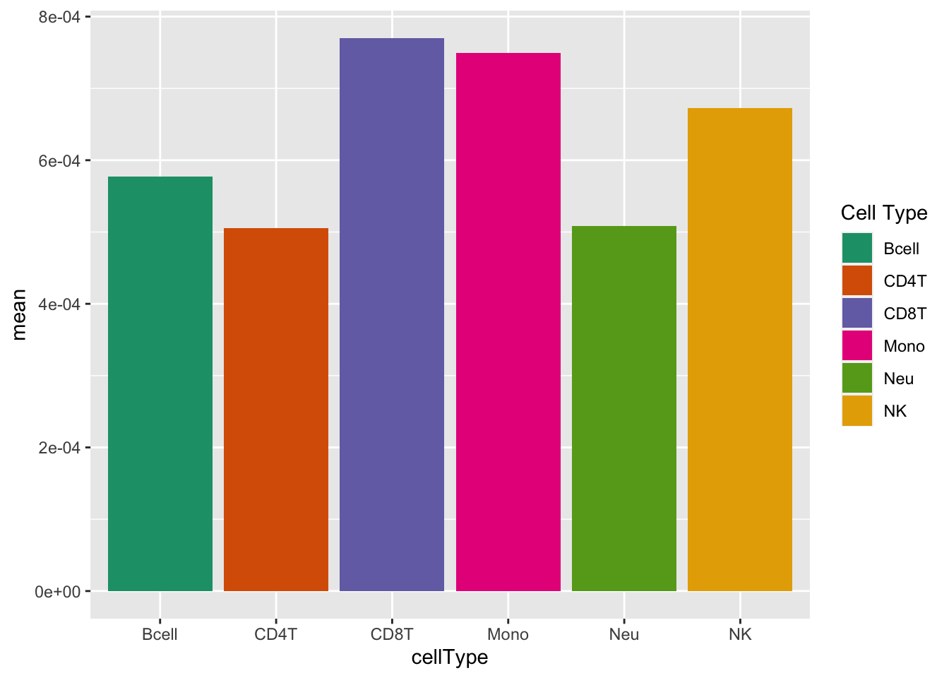
| Version | Author | Date |
|---|---|---|
| 7dac845 | JovMaksimovic | 2021-03-29 |
# plot normalised beta value distribution
bVals <- getBeta(normGr)
dat <- data.frame(reshape2::melt(bVals))
colnames(dat) <- c("cpg", "sample", "bVal")
dat <- dplyr::bind_cols(dat, cellType = rep(targets$CellType,
                                            each = nrow(bVals)))

ggplot(dat, aes(x = bVal, colour = cellType)) +
    geom_density() +
    labs(colour = "Cell Type") +
    scale_color_brewer(palette = "Dark2")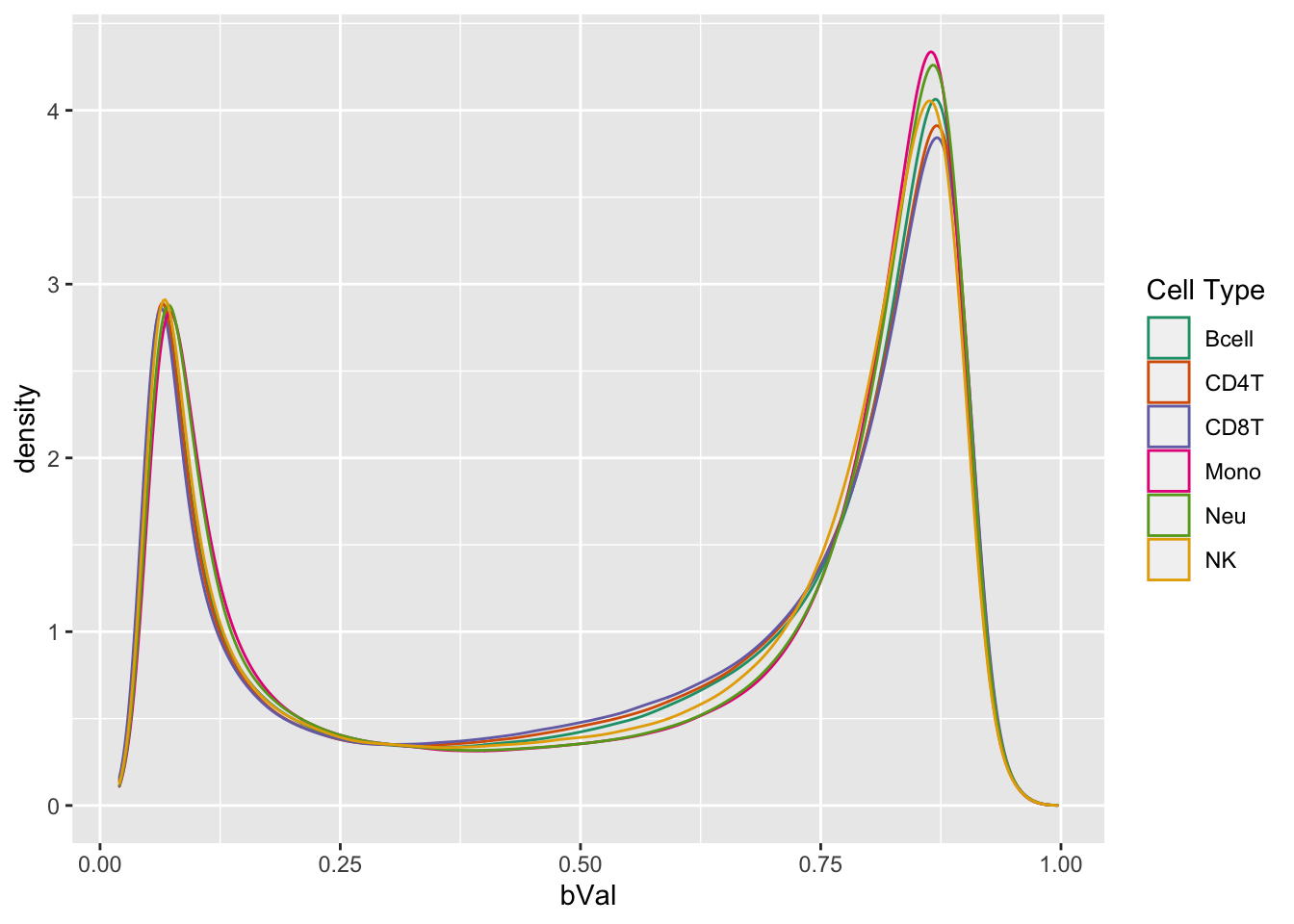
| Version | Author | Date |
|---|---|---|
| 7dac845 | JovMaksimovic | 2021-03-29 |
# MDS plots to look at largest sources of variation
p <- plotMDS(getM(fltGr), top=1000, gene.selection="common", plot = FALSE)
dat <- tibble::tibble(x = p$x, y = p$y, cellType = targets$CellType)

p <- ggplot(dat, aes(x = x, y = y, colour = cellType)) +
    geom_point(size = 2) +
    labs(colour = "Cell type") +
    scale_colour_brewer(palette = "Dark2") +
    labs(x = "Principal component 1", y = "Principal component 2")
p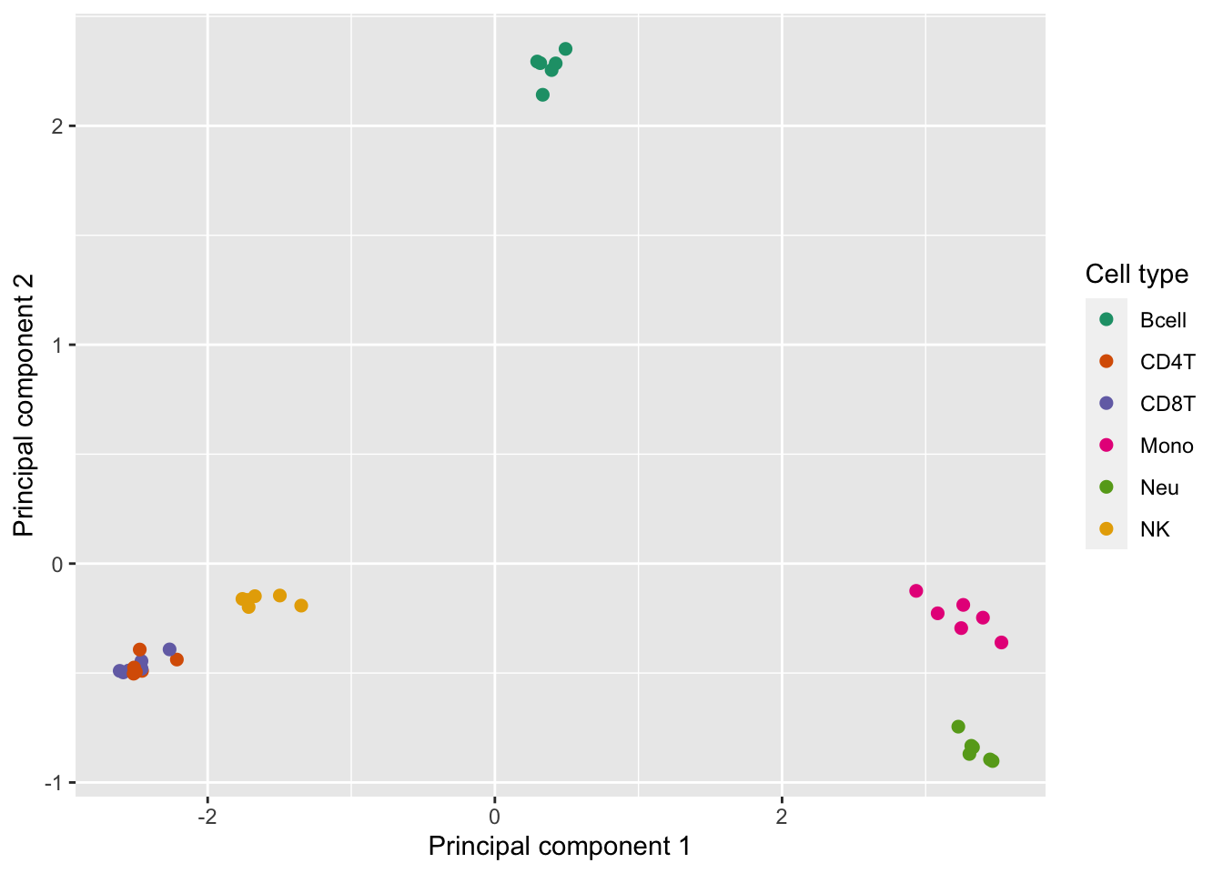
| Version | Author | Date |
|---|---|---|
| 7dac845 | JovMaksimovic | 2021-03-29 |
Save figure for use in manuscript.
outDir <- here::here("output/figures")
if (!dir.exists(outDir)) dir.create(outDir)

fig <- here("output/figures/Fig-4A.rds")
saveRDS(p, fig, compress = FALSE)
Statistical analysis
Compare several sets of sorted immune cells. Consider results significant at FDR < 0.05 and delta beta > 10% (~ lfc = 0.5).
mVals <- getM(fltGr)
bVals <- getBeta(fltGr)
design <- model.matrix(~0+targets$CellType)
colnames(design) <- levels(factor(targets$CellType))
fit <- lmFit(mVals, design)
cont.matrix <- makeContrasts(CD4vCD8=CD4T-CD8T,
MonovNeu=Mono-Neu,
BcellvNK=Bcell-NK,
levels=design)
fit2 <- contrasts.fit(fit, cont.matrix)
tfit <- eBayes(fit2, robust=TRUE, trend=TRUE)
tfit <- treat(tfit, lfc = 0.5)
pval <- 0.05
fitSum <- summary(decideTests(tfit, p.value = pval))
fitSum CD4vCD8 MonovNeu BcellvNK
Down 5072 9324 34803
NotSig 725611 712480 667559
Up 3202 12081 31523bDat <- getBiasDat(rownames(topTreat(tfit, coef = "BcellvNK", num = 5000)),
array.type = "EPIC")All input CpGs are used for testing.p <- ggplot(bDat, aes(x = avgbias, y = propDM)) +
geom_point(shape = 1, size = 2) +
geom_smooth() +
labs(x = "No. CpGs per gene (binned)",
y = "Prop. differential methylation") +
theme_minimal() +
theme(panel.grid = element_blank(),
axis.line = element_line(colour = "black"))
p`geom_smooth()` using method = 'loess' and formula 'y ~ x'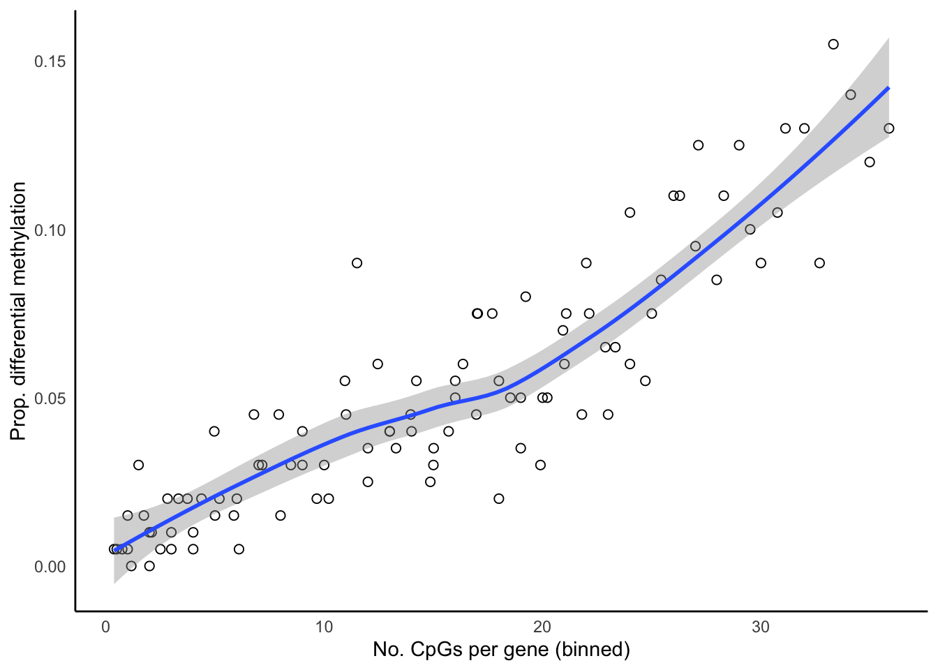
| Version | Author | Date |
|---|---|---|
| 7dac845 | JovMaksimovic | 2021-03-29 |
Save figure for use in manuscript.
fig <- here("output/figures/Fig-1B.rds")
saveRDS(p, fig, compress = FALSE)
Examine only the independent contrasts.
dat <- melt(fitSum[rownames(fitSum) != "NotSig", ])
colnames(dat) <- c("dir","comp","num")

p <- ggplot(dat, aes(x = comp, y = num, fill = dir)) +
    geom_bar(stat = "identity", position = "dodge") +
    labs(x = "Comparison", y = "No. DM CpGs (FDR < 0.05)", fill = "Direction") +
    scale_fill_brewer(palette = "Set1", direction = -1)
p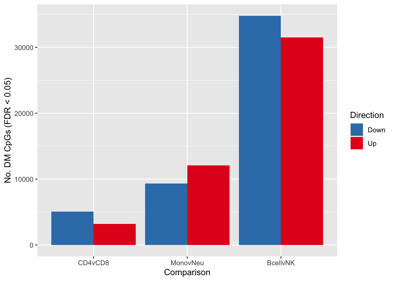
| Version | Author | Date |
|---|---|---|
| 7dac845 | JovMaksimovic | 2021-03-29 |
Save figure for use in manuscript.
fig <- here("output/figures/Fig-4B.rds")
saveRDS(p, fig, compress = FALSE)
Compare performance of different gene set testing methods
We compare the performance of the following gene set testing methods available for methylation arrays: a standard hypergeometric test (HGT), GOmeth from the missMethyl package, methylglm (mGLM), methylRRA-ORA (mRRA (ORA)) and methylRRA-GSEA (mRRA (GSEA)) from the methylGSA package and ebGSEA from GitHub at https://github.com/aet21/ebGSEA.
We perform gene set testing on the results of all three blood cell type comparisons: B-cells vs. NK cells, CD4 T-cells vs. CD8 T-cells and monocytes vs. neutrophils, using all of the different gene set testing methods.
Gene set testing is performed for each comparison using GO categories, KEGG pathways and the BROAD MSigDB gene sets for the following methods: HGT, GOmeth, mGLM, mRRA (ORA), mRRA (GSEA), ebGSEA (WT) and ebGSEA (KPMT).
As the methylGSA methods do not work well with sets that only contain very few genes or very many genes, we only test sets with at least 5 genes and at most 5000 genes.
Firstly, the results of the statistical analysis of the three blood cell comparisons are saved as an RDS object.
minsize <- 5
maxsize <- 5000

outDir <- here::here("data/cache-intermediates")
if (!dir.exists(outDir)) dir.create(outDir)

outFile <- here("data/cache-intermediates/blood.contrasts.rds")

if(!file.exists(outFile)){
  obj <- NULL
  obj$tfit <- tfit
  obj$maxsize <- maxsize
  obj$minsize <- minsize
  obj$mVals <- mVals
  obj$targets <- targets

  saveRDS(obj, file = outFile)

}
As some of the methods take a considerable amount of time to perform the gene set testing analysis, we have created several scripts in order to run the analyses in parallel on a HPC. The code used to run all the gene set testing analyses using the different methods can be found in the code/compare-methods directory. It consists of four scripts: genRunMethodJob.R, runebGSEA.R, runMethylGSA.R and runMissMethyl.R. The genRunMethodJob.R script creates and submits Slurm job scripts that run the runebGSEA.R, runMethylGSA.R and runMissMethyl.R scripts, for each gene set type, in parallel, on a HPC. The results of each job are saved as an RDS file named {package}.{set}.rds in the output/compare-methods/BLOOD directory. Once all analysis jobs are complete, all of the subsequent analyses in this document can be executed.
Load output for all methods
The results of all the gene set testing analyses, using all the different methods, for the different types of gene sets, are loaded into a list of data.frames. All of the data.frames in the list are then concatenated into a tibble for downstream analysis and plotting.
inFiles <- list.files(here("output/compare-methods/BLOOD"), pattern = "rds",
                      full.names = TRUE)

res <- lapply(inFiles, function(file){
    readRDS(file)
})

dat <- as_tibble(dplyr::bind_rows(res))
Explore analysis results
GO categories
Examine the performance of the different methods when gene set testing was performed on GO categories.
ann <- loadAnnotation("EPIC")
flatAnn <- loadFlatAnnotation(ann)
cpgEgGo <- cpgsEgGoFreqs(flatAnn)

cpgEgGo %>%
  group_by(GO) %>%
  summarise(med = median(Freq)) -> medCpgEgGo
In order to examine whether the probe-number bias influenced the significantly enriched GO categories for the different methods, we split the GO categories into bins based on the median number of CpGs per gene per GO category. We then calculated the proportion of significantly enriched GO categories in each bin for each of the three comparisons. As GOmeth explicitly corrects for this bias it showed very little trend. The mGLM method also appears to control for the probe-number bias of the array fairly well. All other methods demonstrated an trend across the different sizes of GO categories.
dat %>% filter(set == "GO") %>%
    filter(sub %in% c("n","c1")) %>%
    mutate(method = unname(dict[method])) %>%
    inner_join(medCpgEgGo, by = c("ID" = "GO")) -> sub

bins <- rbin_quantiles(sub, ID, med, bins = 12)
sub$bin <- as.factor(findInterval(sub$med, bins$upper_cut))

binLabs <- paste0("<", bins$upper_cut)
names(binLabs) <- levels(sub$bin)
binLabs[length(binLabs)] <- gsub("<", "\u2265", binLabs[length(binLabs) - 1])

sub %>% group_by(contrast, method, bin) %>%
  summarise(prop = sum(pvalue < 0.05)/n()) -> pdat
`summarise()` has grouped output by 'contrast', 'method'. You can override using the `.groups` argument.p <- ggplot(pdat, aes(x = as.numeric(bin), y = prop, color = method)) +
geom_line() +
facet_wrap(vars(contrast), ncol = 3) +
scale_x_continuous(breaks = as.numeric(levels(pdat$bin)), labels = binLabs) +
theme(axis.text.x = element_text(angle=45, hjust = 1, vjust = 1,
size = 7),
legend.position = "bottom") +
labs(x = "Med. No. CpGs per Gene per GO Cat. (binned)",
y = "Prop. GO Cat. with p-value < 0.05",
colour = "Method") +
scale_color_manual(values = methodCols)
p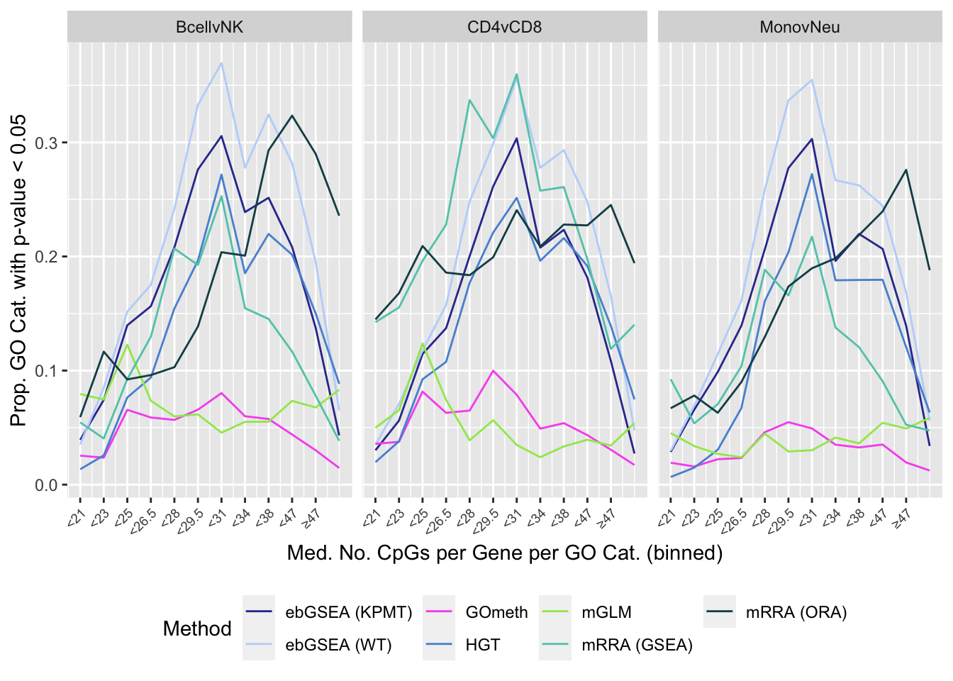
| Version | Author | Date |
|---|---|---|
| 7dac845 | JovMaksimovic | 2021-03-29 |
As we are comparing immune cells, we expect GO categories related to the immune system and its processes to be highly ranked. To evalue this, we downloaded all of the child terms for the GO category "immune system process" (GO:002376) from AminGO 2; http://amigo.geneontology.org/amigo/term/GO:0002376. We also examine results when top ranked 100 GO terms from RNA-seq analysis of the same cell type comparisons is used as "truth".
immuneGO <- unique(read.csv(here("data/genesets/GO-immune-system-process.txt"),
                            stringsAsFactors = FALSE, header = FALSE,
                            col.names = "GOID"))

rnaseqGO <- readRDS(here("data/cache-rnaseq/RNAseq-GO.rds"))
rnaseqGO %>% group_by(contrast) %>%
    mutate(rank = 1:n()) %>%
    filter(rank <= 100) -> topGOSets

p <- vector("list", length(unique(dat$contrast)))

for(i in 1:length(unique(dat$contrast))){
    cont <- sort(unique(dat$contrast))[i]

    dat %>% filter(set == "GO") %>%
        filter(if(cont == "CD4vCD8") sub %in% c("n","p1") else sub %in% c("n","c1")) %>%
        filter(contrast == cont) %>%
        mutate(method = unname(dict[method])) %>%
        arrange(method, pvalue) %>%
        group_by(method) %>%
        mutate(rank = 1:n()) %>%
        filter(rank <= 100) %>%
        mutate(csum = cumsum(ID %in% immuneGO$GOID)) %>%
        mutate(truth = "ISP Terms") -> immuneSum

    dat %>% filter(set == "GO") %>%
        filter(sub %in% c("n","c1")) %>%
        filter(contrast == cont) %>%
        mutate(method = unname(dict[method])) %>%
        arrange(method, pvalue) %>%
        group_by(method) %>%
        mutate(rank = 1:n()) %>%
        filter(rank <= 100) %>%
        mutate(csum = cumsum(ID %in% topGOSets$ID[topGOSets$contrast %in%
                                                         contrast])) %>%
        mutate(truth = "RNAseq Terms") -> rnaseqSum

    truthSum <- bind_rows(immuneSum, rnaseqSum)

    p[[i]] <- ggplot(truthSum, aes(x = rank, y = csum, colour = method)) +
    geom_line() +
    facet_wrap(vars(truth), ncol = 2) +
    geom_vline(xintercept = 10, linetype = "dotted") +
    labs(colour = "Method", x = "Rank",
         y = "Cumulative no. sets in truth") +
    theme(legend.position = "bottom") +
    scale_color_manual(values = methodCols)
}

p[[1]] + ggtitle(sort(unique(dat$contrast))[1])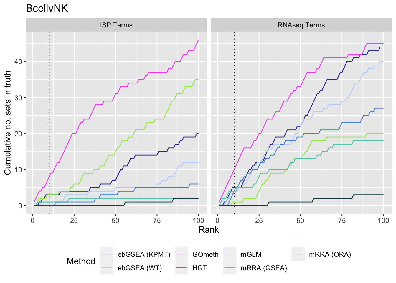
| Version | Author | Date |
|---|---|---|
| 7dac845 | JovMaksimovic | 2021-03-29 |
p[[2]] + ggtitle(sort(unique(dat$contrast))[2])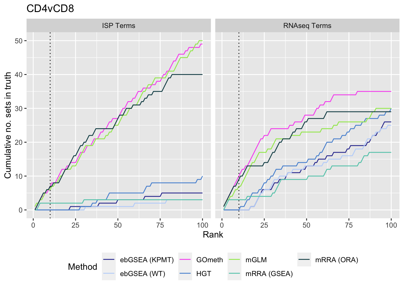
p[[3]] + ggtitle(sort(unique(dat$contrast))[3])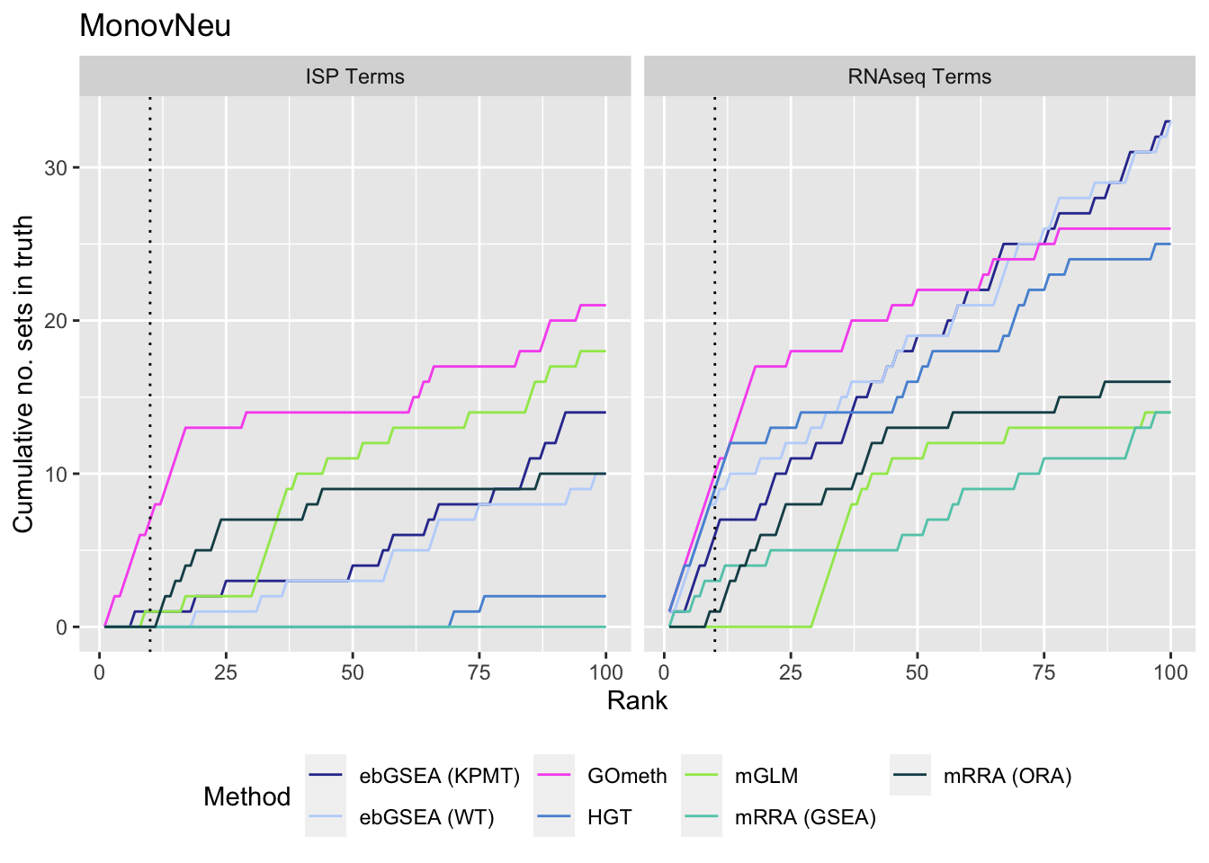
| Version | Author | Date |
|---|---|---|
| 7dac845 | JovMaksimovic | 2021-03-29 |
Save figure for use in manuscript.
fig <- here("output/figures/Fig-4C.rds")
saveRDS(p[[1]], fig, compress = FALSE)

fig <- here("output/figures/SFig-5A.rds")
saveRDS(p[[2]], fig, compress = FALSE)

fig <- here("output/figures/SFig-6A.rds")
saveRDS(p[[3]], fig, compress = FALSE)
Examine what the top 10 ranked gene sets are and how many genes they contain, for each method and comparison.
terms <- missMethyl:::.getGO()$idTable
nGenes <- rownames_to_column(data.frame(n = sapply(missMethyl:::.getGO()$idList,
                                                   length)),
                             var = "ID")

dat %>% filter(set == "GO") %>%
    mutate(method = unname(dict[method])) %>%
    arrange(contrast, method, sub, pvalue) %>%
    group_by(contrast, method, sub) %>%
    mutate(FDR = p.adjust(pvalue, method = "BH")) %>%
    mutate(rank = 1:n()) %>%
    filter(rank <= 10) %>%
    inner_join(terms, by = c("ID" = "GOID")) %>%
    inner_join(nGenes) -> sub
Joining, by = "ID"p <- vector("list", length(unique(sub$contrast)))
truthPal <- scales::hue_pal()(4)
names(truthPal) <- c("Both", "ISP", "Neither", "RNAseq")
for(i in 1:length(p)){
cont <- sort(unique(sub$contrast))[i]
sub %>% filter(contrast == cont) %>%
filter(if(cont == "CD4vCD8") sub %in% c("n","p1") else sub %in% c("n","c1")) %>%
arrange(method, -rank) %>%
ungroup() %>%
mutate(idx = as.factor(1:n())) -> tmp
setLabs <- substr(tmp$TERM, 1, 40)
names(setLabs) <- tmp$idx
tmp %>% mutate(rna = ID %in% topGOSets$ID[topGOSets$contrast %in% cont],
isp = ID %in% immuneGO$GOID,
both = rna + isp,
col = ifelse(both == 2, "Both",
ifelse(both == 1 & rna == 1, "RNAseq",
ifelse(both == 1 & isp == 1,
"ISP", "Neither")))) %>%
mutate(col = factor(col,
levels = c("Both", "ISP", "RNAseq",
"Neither"))) -> tmp
p[[i]] <- ggplot(tmp, aes(x = -log10(FDR), y = idx, colour = col)) +
geom_point(aes(size = n), alpha = 0.7) +
scale_size(limits = c(min(sub$n), max(sub$n))) +
facet_wrap(vars(method), ncol = 2, scales = "free") +
scale_y_discrete(labels = setLabs) +
scale_colour_manual(values = truthPal) +
labs(y = "", size = "No. genes", colour = "In truth set") +
theme(axis.text.y = element_text(size = 6),
axis.text.x = element_text(size = 6),
legend.box = "horizontal",
legend.margin = margin(0, 0, 0, 0, unit = "lines"),
panel.spacing.x = unit(1, "lines")) +
coord_cartesian(xlim = c(-log10(0.99), -log10(10^-300))) +
geom_vline(xintercept = -log10(0.05), linetype = "dashed") +
ggtitle(cont)
}
shift_legend(p[[1]], plot = TRUE, pos = "left")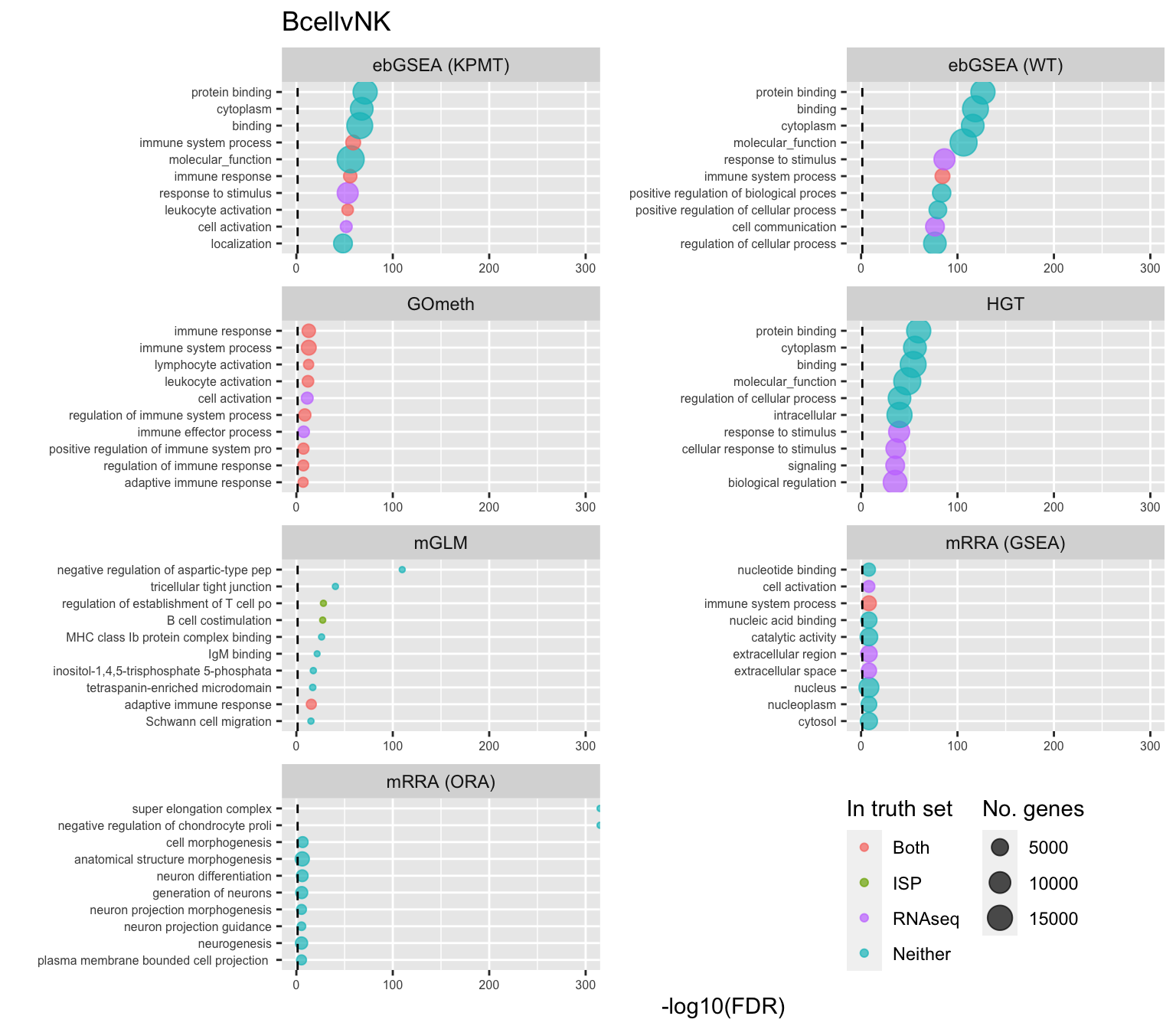
shift_legend(p[[2]], plot = TRUE, pos = "left")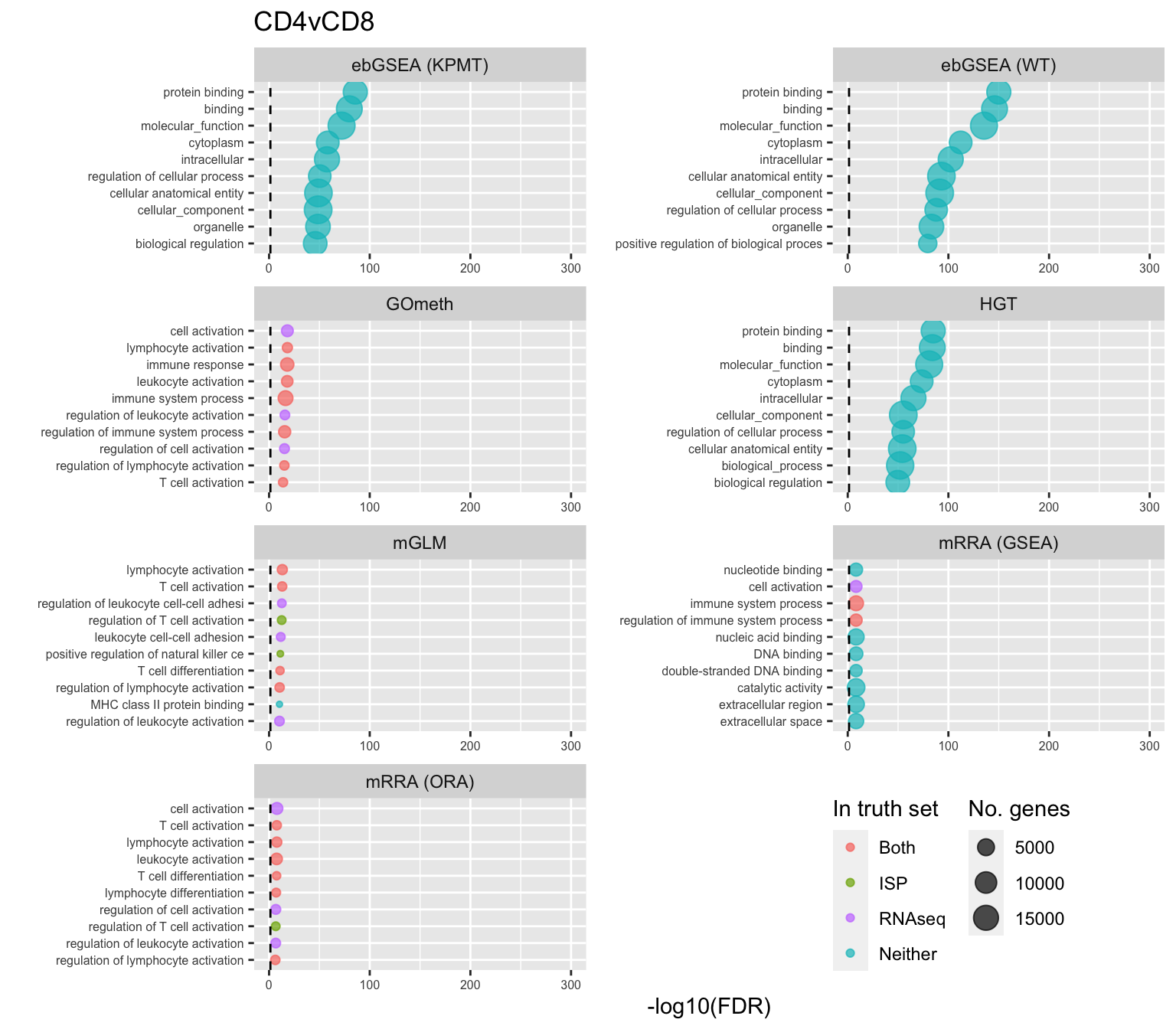
shift_legend(p[[3]], plot = TRUE, pos = "left")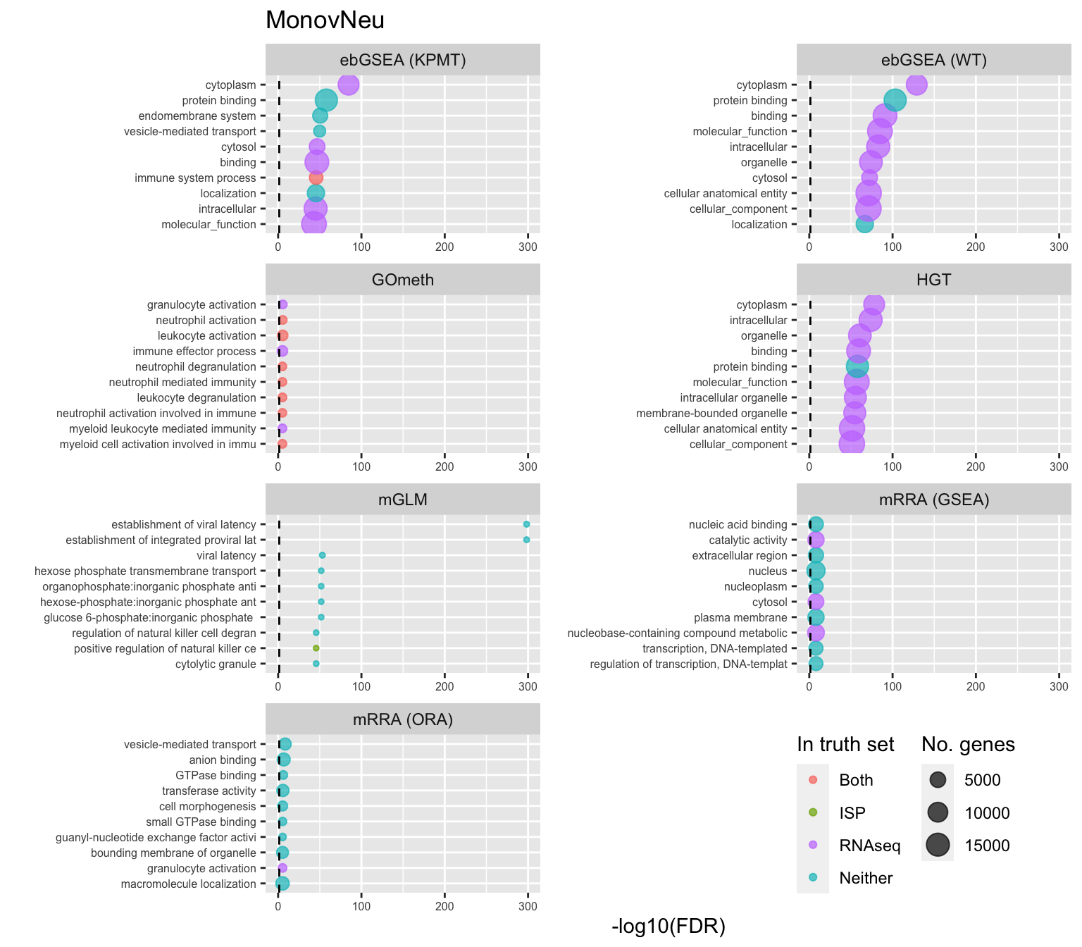
Save figure for use in manuscript.
fig <- here("output/figures/Fig-4D.rds")
saveRDS(shift_legend(p[[1]] + theme(plot.title = element_blank()),
                     pos = "left"),
        fig, compress = FALSE)

fig <- here("output/figures/SFig-5B.rds")
saveRDS(shift_legend(p[[2]] + theme(plot.title = element_blank()),
                     pos = "left"),
        fig, compress = FALSE)

fig <- here("output/figures/SFig-6B.rds")
saveRDS(shift_legend(p[[3]] + theme(plot.title = element_blank()),
                     pos = "left"),
        fig, compress = FALSE)
P-value histograms for the different methods for all contrasts on GO categories.
dat %>% filter(set == "GO") %>%
    filter(sub %in% c("n","c1")) %>%
    mutate(method = unname(dict[method])) -> subDat

ggplot(subDat, aes(pvalue, fill = method)) +
    geom_histogram(binwidth = 0.025) +
    facet_grid(cols = vars(contrast), rows = vars(method)) +
    theme(legend.position = "bottom") +
    labs(x = "P-value", y = "Frequency", fill = "Method") +
    scale_fill_manual(values = methodCols)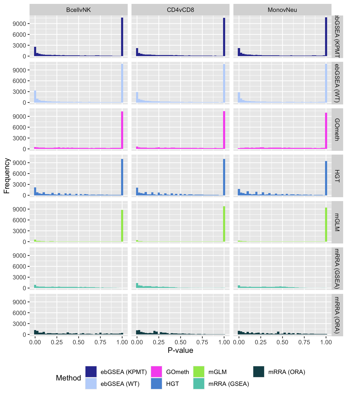
| Version | Author | Date |
|---|---|---|
| 7dac845 | JovMaksimovic | 2021-03-29 |
Compare GOmeth results using different DM CpG significance cutoffs
As the results of GOmeth depend on the list of significant CpGs provided as input to the function, we explored the effect of selecting "significant" CpGs in different ways on the gene set testing performance of GOmeth.
dat %>% filter(set == "GO") %>%
    filter(grepl("mmethyl", method)) %>%
    mutate(method = unname(dict[method])) %>%
    arrange(contrast, method, pvalue) %>%
    group_by(contrast, method, sub) %>%
    mutate(csum = cumsum(ID %in% immuneGO$GOID)) %>%
    mutate(rank = 1:n()) %>%
    mutate(cut = ifelse(sub == "c1", "Top 5000",
                        ifelse(sub == "c2", "Top 10000",
                               ifelse(sub == "p1", "FDR < 0.01", "FDR < 0.05")))) %>%
    filter(rank <= 100) -> sub

p <- ggplot(sub, aes(x = rank, y = csum, colour = cut)) +
    geom_line() +
    facet_wrap(vars(contrast, method), ncol=2, nrow = 3, scales = "free") +
    geom_vline(xintercept = 10, linetype = "dotted") +
    labs(colour = "Sig. select", x = "Rank", y = "Cumulative no. immune sets") +
    theme(legend.position = "bottom")
p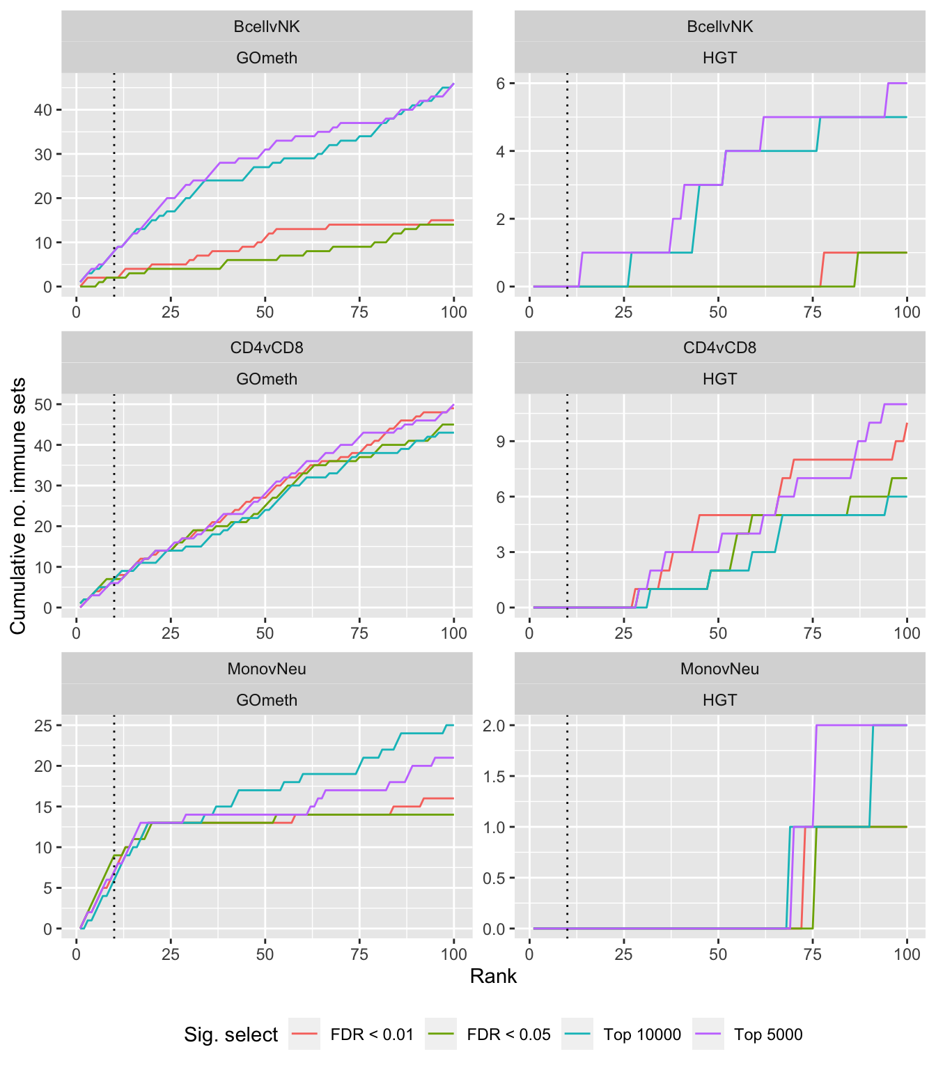
| Version | Author | Date |
|---|---|---|
| 7dac845 | JovMaksimovic | 2021-03-29 |
dat %>% filter(set == "GO") %>%
    filter(grepl("mmethyl", method)) %>%
    mutate(method = unname(dict[method])) %>%
    arrange(contrast, method, pvalue) %>%
    group_by(contrast, method, sub) %>%
    mutate(csum = cumsum(ID %in% topGOSets$ID[topGOSets$contrast %in%
                                                  contrast])) %>%
    mutate(rank = 1:n()) %>%
    mutate(cut = ifelse(sub == "c1", "Top 5000",
                        ifelse(sub == "c2", "Top 10000",
                               ifelse(sub == "p1", "FDR < 0.01", "FDR < 0.05")))) %>%
    filter(rank <= 100) -> sub

p <- ggplot(sub, aes(x = rank, y = csum, colour = cut)) +
    geom_line() +
    facet_wrap(vars(contrast, method), ncol=2, nrow = 3, scales = "free") +
    geom_vline(xintercept = 10, linetype = "dotted") +
    labs(colour = "Sig. select", x = "Rank",
         y = glue("Cumulative no. RNAseq sets")) +
    theme(legend.position = "bottom")
p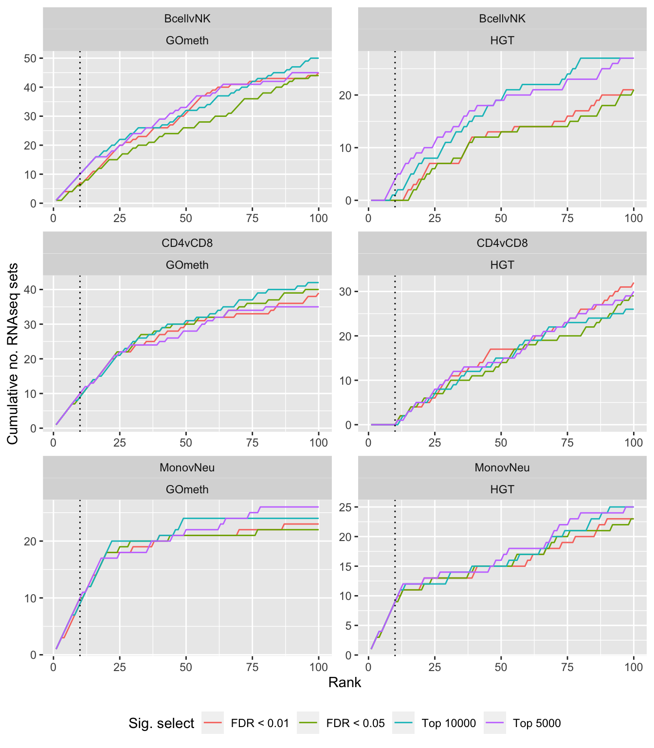
| Version | Author | Date |
|---|---|---|
| 7dac845 | JovMaksimovic | 2021-03-29 |
KEGG pathways
Now test KEGG pathways with at least 5 genes and 5000 at most.
Again, as we are comparing immune cells we expect pathways from the following categories to be highly ranked: Immune system, Immune disease, Signal transduction, Signaling molecules and interaction; https://www.genome.jp/kegg/pathway.html.
immuneKEGG <- read.csv(here("data/genesets/kegg-immune-related-pathways.csv"),
                            stringsAsFactors = FALSE, header = FALSE,
                            col.names = c("ID","pathway"))
immuneKEGG$PID <- paste0("path:hsa0",immuneKEGG$ID)

rnaseqKEGG <- readRDS(here("data/cache-rnaseq/RNAseq-KEGG.rds"))
rnaseqKEGG %>% group_by(contrast) %>%
    mutate(rank = 1:n()) %>%
    filter(rank <= 100) -> topKEGG

p1 <- vector("list", length(unique(dat$contrast)))

for(i in 1:length(unique(dat$contrast))){
    cont <- sort(unique(dat$contrast))[i]

    dat %>% filter(set == "KEGG") %>%
        filter(if(cont == "CD4vCD8") sub %in% c("n","p1") else sub %in% c("n","c1")) %>%
        filter(contrast == cont) %>%
        mutate(method = unname(dict[method])) %>%
        arrange(method, pvalue) %>%
        group_by(method) %>%
        mutate(rank = 1:n()) %>%
        filter(rank <= 100) %>%
        mutate(csum = cumsum(ID %in% immuneKEGG$PID)) %>%
        mutate(truth = "ISP Terms") -> immuneSum

    p1[[i]] <- ggplot(immuneSum, aes(x = rank, y = csum, colour = method)) +
    geom_line() +
    facet_wrap(vars(contrast), nrow = 1, ncol = 1) +
    geom_vline(xintercept = 10, linetype = "dotted") +
    labs(colour = "Method", x = "Rank",
         y = "Cumulative no. immune sets") +
    theme(legend.position = "bottom") +
    scale_color_manual(values = methodCols)
}

p2 <- vector("list", length(unique(dat$contrast)))

for(i in 1:length(unique(dat$contrast))){
    cont <- sort(unique(dat$contrast))[i]

    dat %>% filter(set == "KEGG") %>%
        filter(if(cont == "CD4vCD8") sub %in% c("n","p1") else sub %in% c("n","c1")) %>%
        filter(contrast == cont) %>%
        mutate(method = unname(dict[method])) %>%
        arrange(method, pvalue) %>%
        group_by(method) %>%
        mutate(rank = 1:n()) %>%
        filter(rank <= 100) %>%
        mutate(csum = cumsum(ID %in% topKEGG$PID[topKEGG$contrast %in%
                                                         cont])) %>%
        mutate(truth = "RNAseq Terms") -> rnaseqSum

    p2[[i]] <- ggplot(rnaseqSum, aes(x = rank, y = csum, colour = method)) +
    geom_line() +
    facet_wrap(vars(contrast), nrow = 1, ncol = 1) +
    geom_vline(xintercept = 10, linetype = "dotted") +
    labs(colour = "Method", x = "Rank",
         y = "Cumulative no. RNAseq sets") +
    theme(legend.position = "bottom") +
    scale_color_manual(values = methodCols)
}

p1 <- (p1[[1]] | p1[[2]] + theme(axis.title.y = element_blank()) |
        p1[[3]] + theme(axis.title.y = element_blank()))
p2 <- (p2[[1]] | p2[[2]] + theme(axis.title.y = element_blank()) |
        p2[[3]] + theme(axis.title.y = element_blank()))

(p1 / p2) + plot_layout(guides = "collect") &
    theme(legend.position = "right")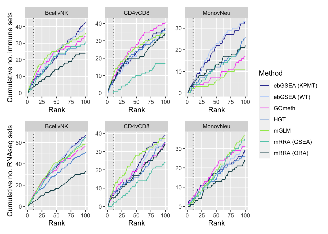
| Version | Author | Date |
|---|---|---|
| 4c57176 | JovMaksimovic | 2021-04-13 |
Save figure for use in manuscript.
fig <- here("output/figures/SFig-7A.rds")
saveRDS(p1, fig, compress = FALSE)

fig <- here("output/figures/SFig-7B.rds")
saveRDS(p2, fig, compress = FALSE)
Examine what the top 10 ranked gene sets are and how many genes they contain, for each method and comparison.
terms <- missMethyl:::.getKEGG()$idTable
nGenes <- rownames_to_column(data.frame(n = sapply(missMethyl:::.getKEGG()$idList,
                                                   length)),
                             var = "ID")

dat %>% filter(set == "KEGG") %>%
   # filter(sub %in% c("n","c1")) %>%
    mutate(method = unname(dict[method])) %>%
    arrange(contrast, method, sub, pvalue) %>%
    group_by(contrast, method, sub) %>%
    mutate(FDR = p.adjust(pvalue, method = "BH")) %>%
    mutate(rank = 1:n()) %>%
    filter(rank <= 10) %>%
    inner_join(terms, by = c("ID" = "PathwayID")) %>%
    inner_join(nGenes) -> sub
Joining, by = "ID"p <- vector("list", length(unique(sub$contrast)))
for(i in 1:length(p)){
cont <- sort(unique(sub$contrast))[i]
sub %>% filter(contrast == cont) %>%
filter(if(cont == "CD4vCD8") sub %in% c("n","p1") else sub %in% c("n","c1")) %>%
arrange(method, -rank) %>%
ungroup() %>%
mutate(idx = as.factor(1:n())) -> tmp
setLabs <- substr(tmp$Description, 1, 40)
names(setLabs) <- tmp$idx
tmp %>% mutate(rna = ID %in% topKEGG$PID[topKEGG$contrast %in% cont],
isp = ID %in% immuneKEGG$PID,
both = rna + isp,
col = ifelse(both == 2, "Both",
ifelse(both == 1 & rna == 1, "RNAseq",
ifelse(both == 1 & isp == 1,
"ISP", "Neither")))) %>%
mutate(col = factor(col,
levels = c("Both", "ISP", "RNAseq",
"Neither"))) -> tmp
p[[i]] <- ggplot(tmp, aes(x = -log10(FDR), y = idx, colour = col)) +
geom_point(aes(size = n), alpha = 0.7) +
scale_size(limits = c(min(sub$n), max(sub$n))) +
facet_wrap(vars(method), ncol = 2, scales = "free") +
scale_y_discrete(labels = setLabs) +
scale_colour_manual(values = truthPal) +
labs(y = "", size = "No. genes", colour = "In truth set") +
theme(axis.text.y = element_text(size = 6),
axis.text.x = element_text(size = 6),
legend.box = "horizontal",
legend.margin = margin(0, 0, 0, 0, unit = "lines"),
panel.spacing.x = unit(1, "lines")) +
coord_cartesian(xlim = c(-log10(0.99), -log10(10^-80))) +
geom_vline(xintercept = -log10(0.05), linetype = "dashed") +
ggtitle(cont)
}
shift_legend(p[[1]], plot = TRUE, pos = "left")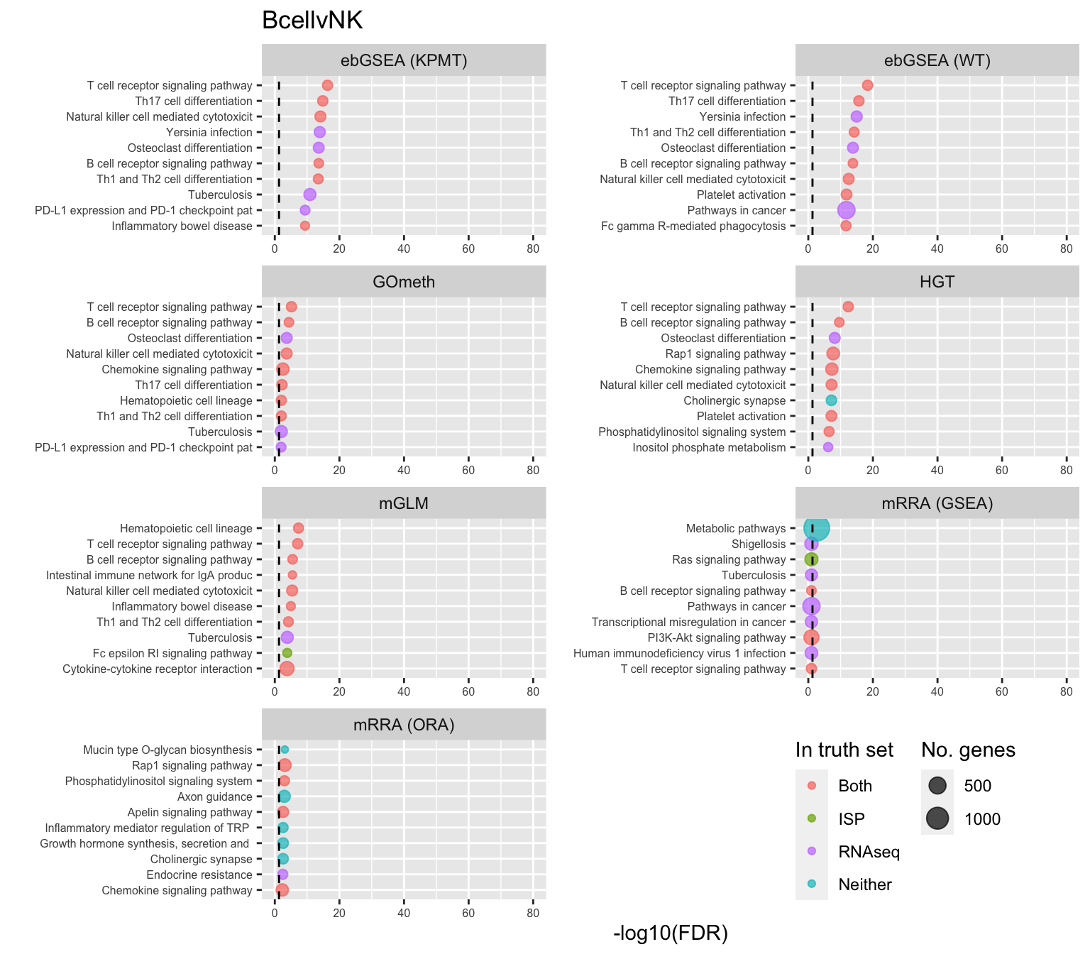
| Version | Author | Date |
|---|---|---|
| 4c57176 | JovMaksimovic | 2021-04-13 |
shift_legend(p[[2]], plot = TRUE, pos = "left")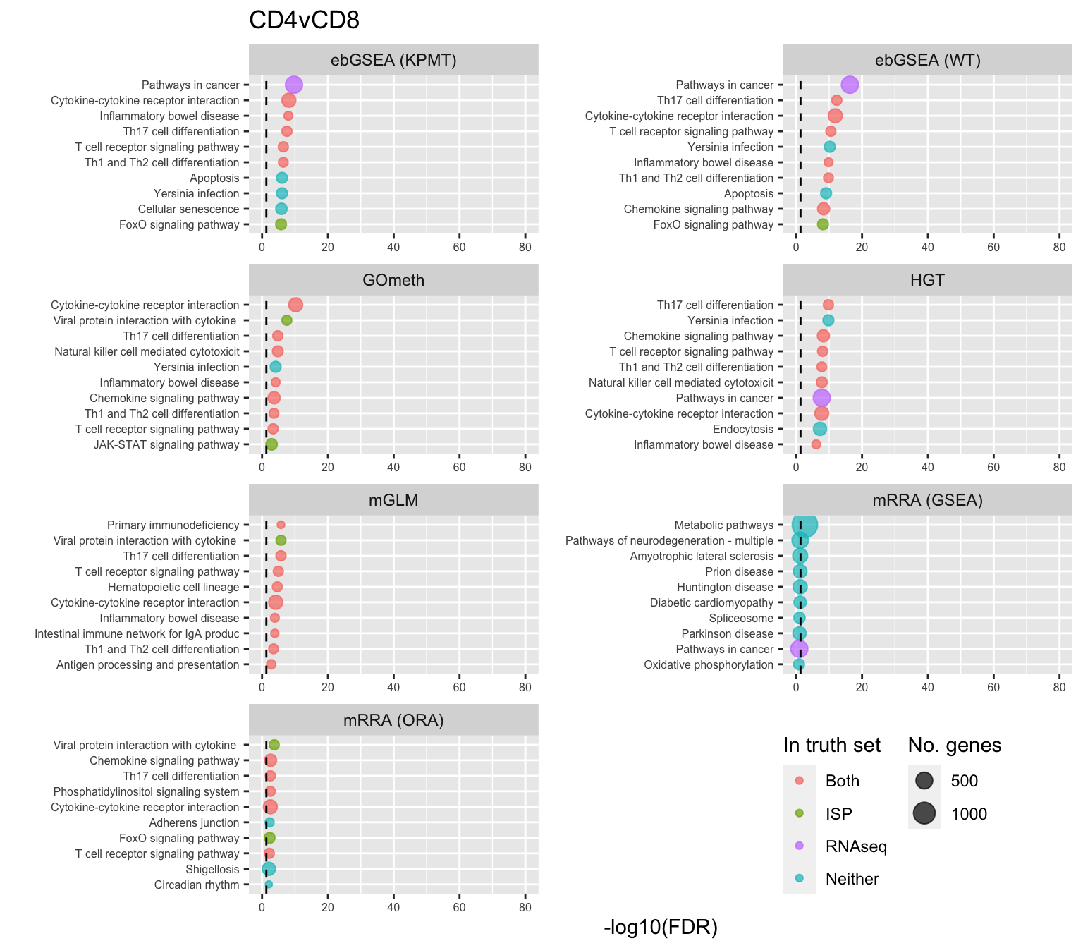
| Version | Author | Date |
|---|---|---|
| 4c57176 | JovMaksimovic | 2021-04-13 |
shift_legend(p[[3]], plot = TRUE, pos = "left")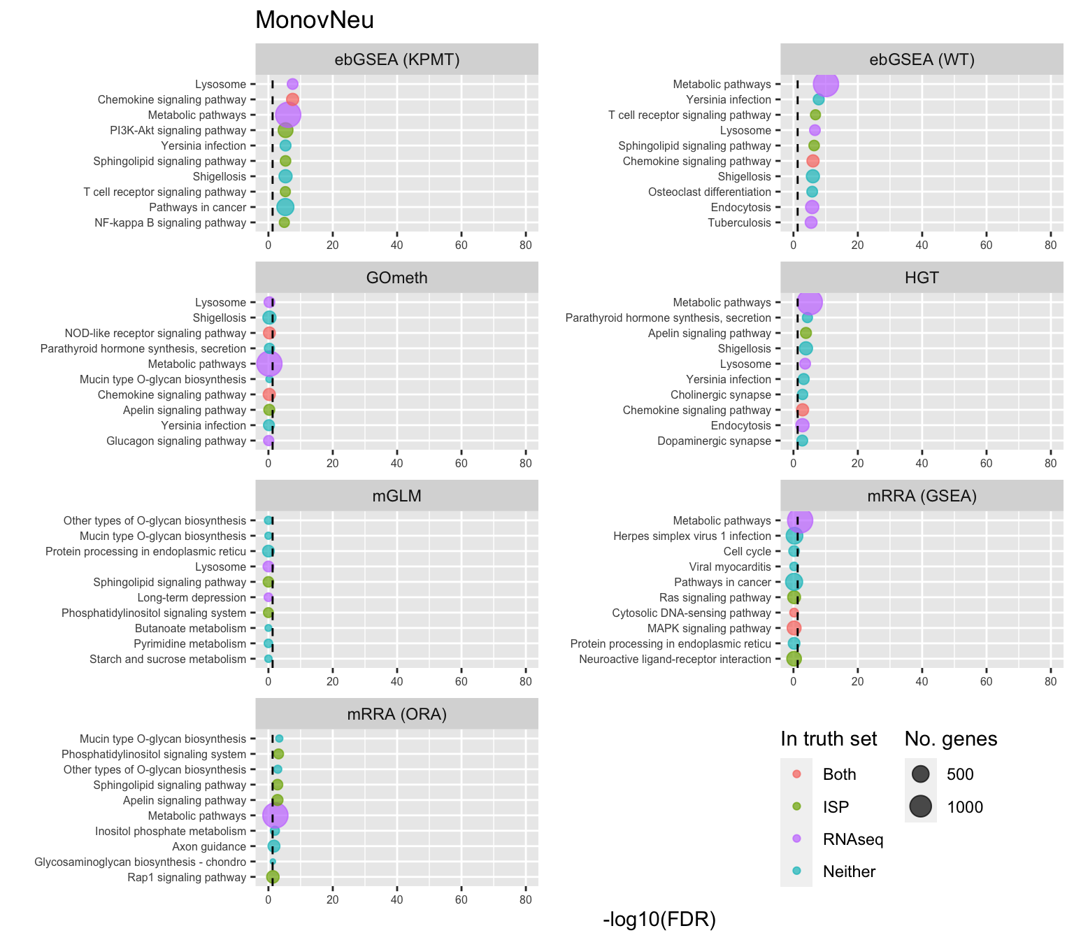
| Version | Author | Date |
|---|---|---|
| 4c57176 | JovMaksimovic | 2021-04-13 |
Save figure for use in manuscript.
fig <- here("output/figures/SFig-7C.rds")
saveRDS(shift_legend(p[[1]] + theme(plot.title = element_blank()),
                     pos = "left"),
        fig, compress = FALSE)

fig <- here("output/figures/SFig-7D.rds")
saveRDS(shift_legend(p[[2]] + theme(plot.title = element_blank()),
                     pos = "left"),
        fig, compress = FALSE)

fig <- here("output/figures/SFig-7E.rds")
saveRDS(shift_legend(p[[3]] + theme(plot.title = element_blank()),
                     pos = "left"),
        fig, compress = FALSE)
P-value histograms for the different methods for all contrasts on KEGG pathways.
dat %>% filter(set == "KEGG") %>%
    filter(sub %in% c("n","c1")) %>%
    mutate(method = unname(dict[method])) -> subDat

ggplot(subDat, aes(pvalue, fill = method)) +
    geom_histogram(binwidth = 0.025) +
    facet_grid(cols = vars(contrast), rows = vars(method)) +
    theme(legend.position = "bottom") +
    labs(x = "P-value", y = "Frequency", fill = "Method") +
    scale_fill_manual(values = methodCols)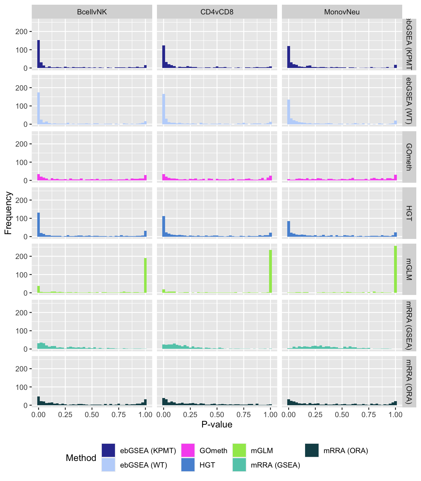
| Version | Author | Date |
|---|---|---|
| 4c57176 | JovMaksimovic | 2021-04-13 |
Compare GOmeth results using different DM CpG significance cutoffs
As the results of GOmeth depend on the list of significant CpGs provided as input to the function, we explored the effect of selecting "significant" CpGs in different ways on the gene set testing performance of GOmeth.
dat %>% filter(set == "KEGG") %>%
    filter(grepl("mmethyl", method)) %>%
    mutate(method = unname(dict[method])) %>%
    arrange(contrast, method, pvalue) %>%
    group_by(contrast, method, sub) %>%
    mutate(csum = cumsum(ID %in% immuneKEGG$PID)) %>%
    mutate(rank = 1:n()) %>%
    mutate(cut = ifelse(sub == "c1", "Top 5000",
                        ifelse(sub == "c2", "Top 10000",
                               ifelse(sub == "p1", "FDR < 0.01", "FDR < 0.05")))) %>%
    filter(rank <= 100) -> sub

p <- ggplot(sub, aes(x = rank, y = csum, colour = cut)) +
    geom_line() +
    facet_wrap(vars(contrast, method), ncol=2, nrow = 3, scales = "free") +
    geom_vline(xintercept = 10, linetype = "dotted") +
    labs(colour = "Sig. select", x = "Rank", y = "Cumulative no. immune sets") +
    theme(legend.position = "bottom")
p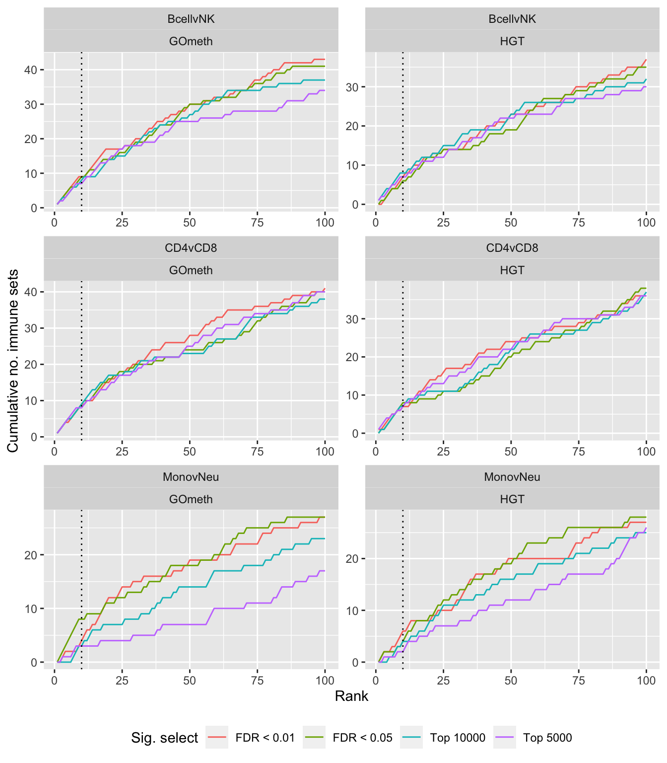
dat %>% filter(set == "KEGG") %>%
    filter(grepl("mmethyl", method)) %>%
    mutate(method = unname(dict[method])) %>%
    arrange(contrast, method, pvalue) %>%
    group_by(contrast, method, sub) %>%
    mutate(csum = cumsum(ID %in% topKEGG$PID[topKEGG$contrast %in% contrast])) %>%
    mutate(rank = 1:n()) %>%
    mutate(cut = ifelse(sub == "c1", "Top 5000",
                        ifelse(sub == "c2", "Top 10000",
                               ifelse(sub == "p1", "FDR < 0.01", "FDR < 0.05")))) %>%
    filter(rank <= 100) -> sub

p <- ggplot(sub, aes(x = rank, y = csum, colour = cut)) +
    geom_line() +
    facet_wrap(vars(contrast, method), ncol=2, nrow = 3, scales = "free") +
    geom_vline(xintercept = 10, linetype = "dotted") +
    labs(colour = "Sig. select", x = "Rank",
         y = glue("Cumulative no. RNAseq sets")) +
    theme(legend.position = "bottom")
p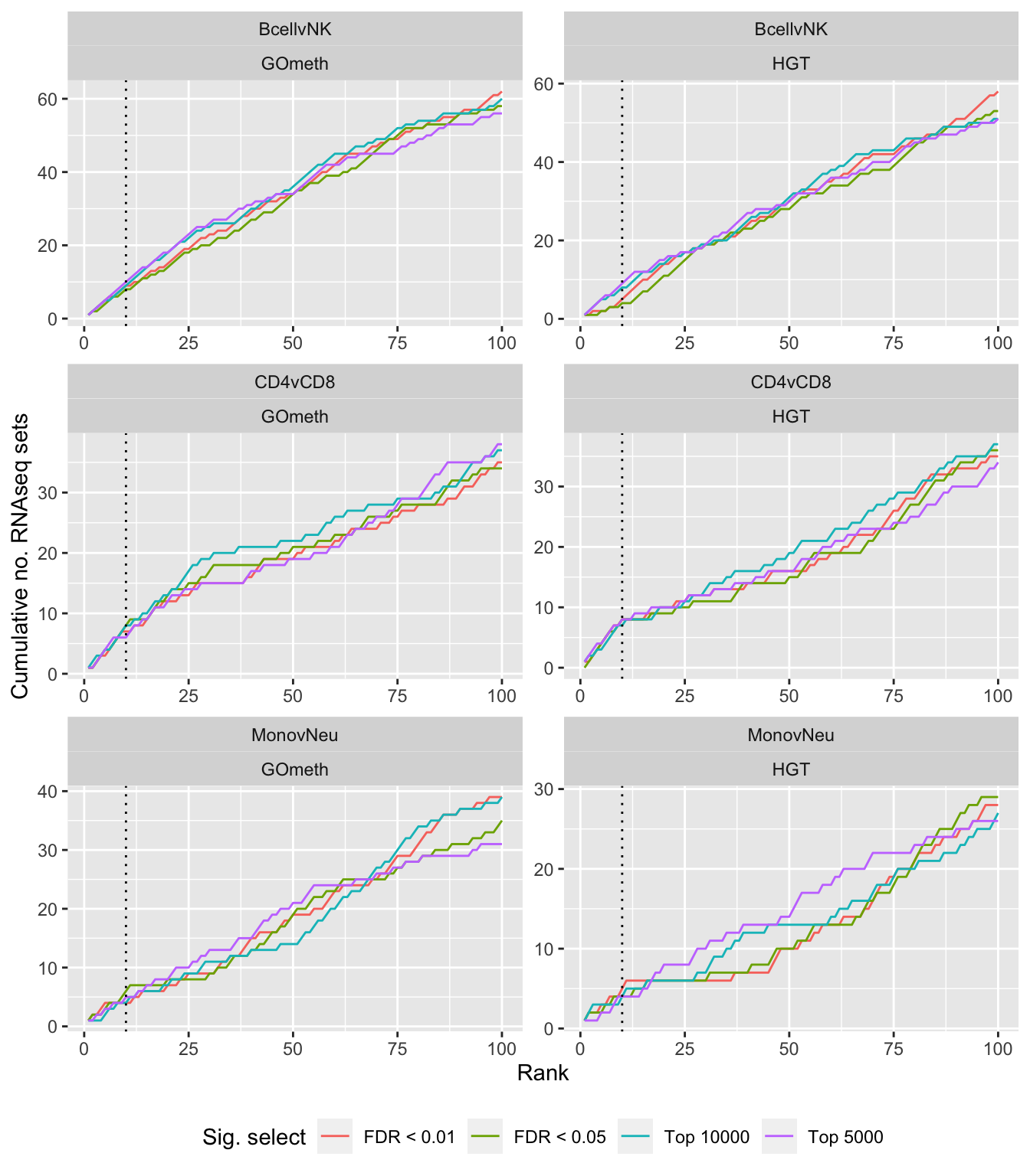
BROAD gene sets
Compare methods by testing the in-built database of Broad Institute gene sets provided with the ChAMP. Using the top 100 ranked gene sets as identified by gsaseq analysis of the corresponding B-cell development stages data as "truth".
rnaseqBROAD <- readRDS(here("data/cache-rnaseq/RNAseq-BROAD-GSA.rds"))
rnaseqBROAD %>% group_by(contrast) %>%
    mutate(rank = 1:n()) %>%
    filter(rank <= 100) -> topBROAD

p <- vector("list", length(unique(dat$contrast)))

for(i in 1:length(unique(dat$contrast))){
    cont <- sort(unique(dat$contrast))[i]

    dat %>% filter(set == "BROAD") %>%
        filter(sub %in% c("n","c1")) %>%
        filter(contrast == cont) %>%
        mutate(method = unname(dict[method])) %>%
    arrange(contrast, method, pvalue) %>%
    group_by(contrast, method) %>%
    mutate(csum = cumsum(ID %in% topBROAD$ID[topBROAD$contrast %in% contrast])) %>%
    mutate(rank = 1:n()) %>%
    filter(rank <= 100) -> sub

    p[[i]] <- ggplot(sub, aes(x = rank, y = csum, colour = method)) +
    geom_line() +
    geom_vline(xintercept = 10, linetype = "dotted") +
    labs(colour = "Method", x = "Rank", y = "Cumulative no. RNAseq sets") +
    theme(legend.position = "bottom") +
    scale_color_manual(values = methodCols) +
        ggtitle(cont)
}

p[[1]]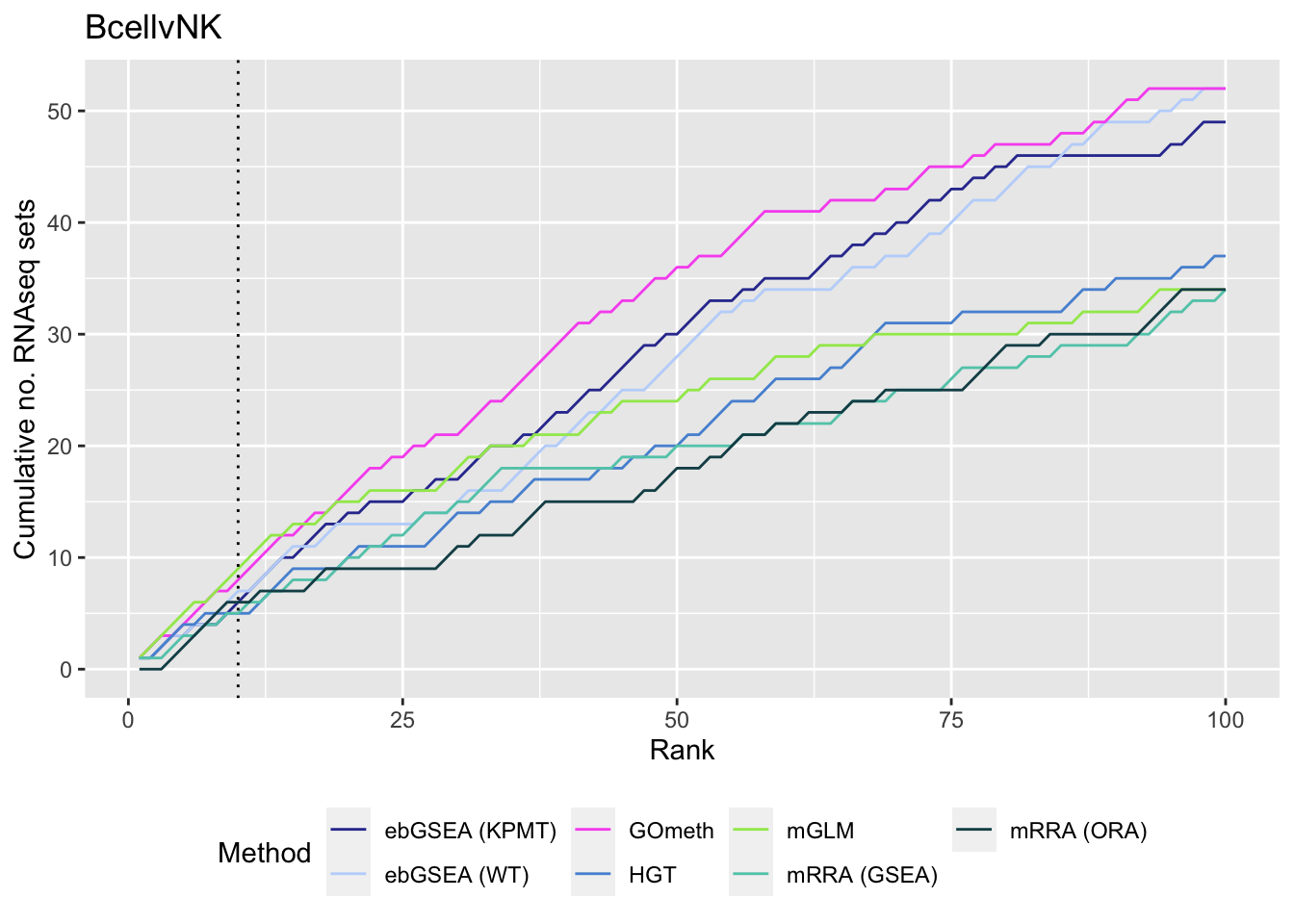
p[[2]]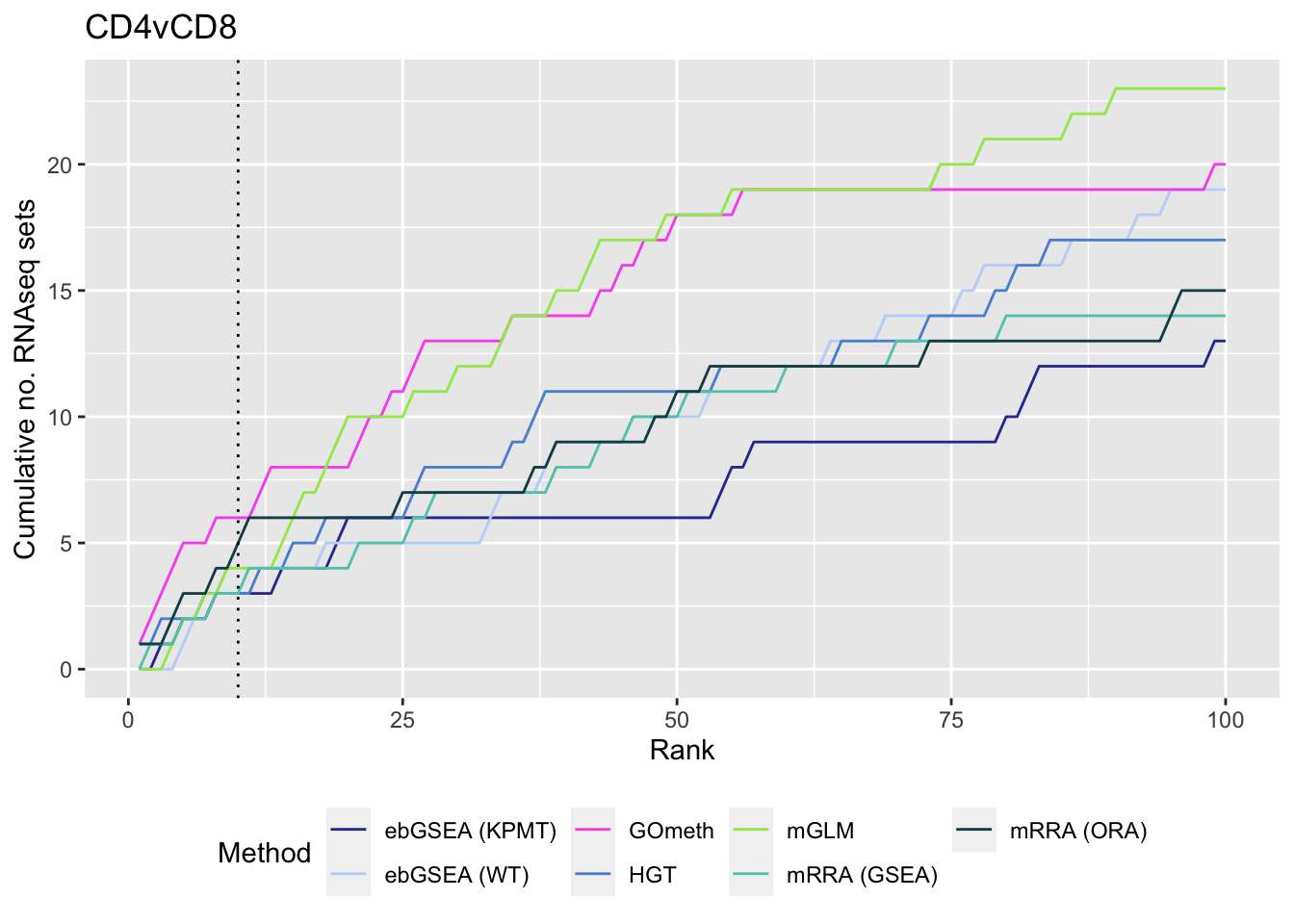
| Version | Author | Date |
|---|---|---|
| 4c57176 | JovMaksimovic | 2021-04-13 |
p[[3]]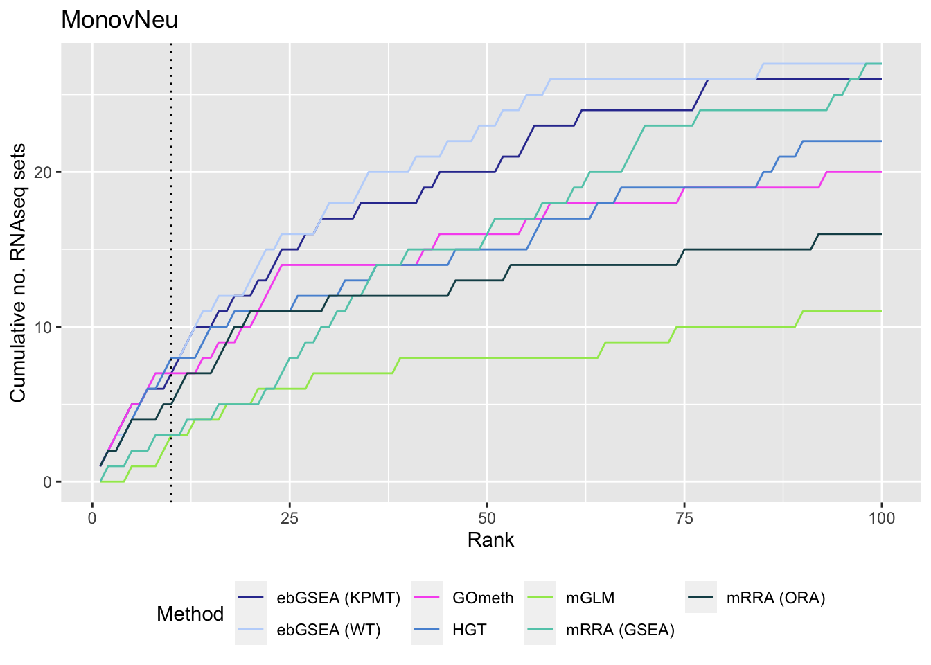
| Version | Author | Date |
|---|---|---|
| 4c57176 | JovMaksimovic | 2021-04-13 |
Examine what the top 10 ranked gene sets are and how many genes they contain, for each method and comparison.
data(PathwayList)
nGenes <- rownames_to_column(data.frame(n = sapply(PathwayList,
                                                   length)),
                             var = "ID")

dat %>% filter(set == "BROAD") %>%
    filter(sub %in% c("n","c1")) %>%
    mutate(method = unname(dict[method])) %>%
    arrange(contrast, method, pvalue) %>%
    group_by(contrast, method) %>%
    mutate(FDR = p.adjust(pvalue, method = "BH")) %>%
    mutate(rank = 1:n()) %>%
    filter(rank <= 10) %>%
    inner_join(nGenes) -> sub
Joining, by = "ID"truthPal <- scales::hue_pal()(4)[3:4]
names(truthPal) <- c("None", "RNAseq")
p <- vector("list", length(unique(sub$contrast)))
for(i in 1:length(p)){
cont <- sort(unique(sub$contrast))[i]
sub %>% filter(contrast == cont) %>%
arrange(method, -rank) %>%
ungroup() %>%
mutate(idx = as.factor(1:n())) -> tmp
setLabs <- substr(tmp$ID, 1, 30)
names(setLabs) <- tmp$idx
tmp %>% mutate(rna = ID %in% topBROAD$ID[topGOSets$contrast %in% cont],
col = ifelse(rna == 1, "RNAseq", "None")) %>%
mutate(col = factor(col, levels = c("RNAseq", "None"))) -> tmp
p[[i]] <- ggplot(tmp, aes(x = -log10(FDR), y = idx, colour = col)) +
geom_point(aes(size = n), alpha = 0.7) +
scale_size(limits = c(min(sub$n), max(sub$n))) +
facet_wrap(vars(method), ncol = 2, scales = "free") +
scale_y_discrete(labels = setLabs) +
scale_color_manual(values = truthPal) +
labs(y = "", size = "No. genes", colour = "In truth set") +
theme(axis.text.y = element_text(size = 6),
axis.text.x = element_text(size = 6),
legend.box = "horizontal",
legend.margin = margin(0, 0, 0, 0, unit = "lines"),
panel.spacing.x = unit(1, "lines")) +
coord_cartesian(xlim = c(-log10(0.99), -log10(10^-100))) +
geom_vline(xintercept = -log10(0.05), linetype = "dashed") +
ggtitle(cont)
}
shift_legend(p[[1]], plot = TRUE, pos = "left")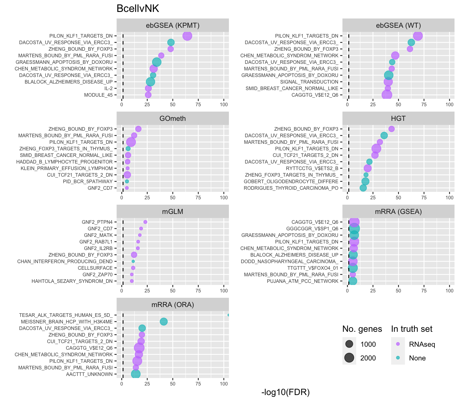
| Version | Author | Date |
|---|---|---|
| 4c57176 | JovMaksimovic | 2021-04-13 |
shift_legend(p[[2]], plot = TRUE, pos = "left")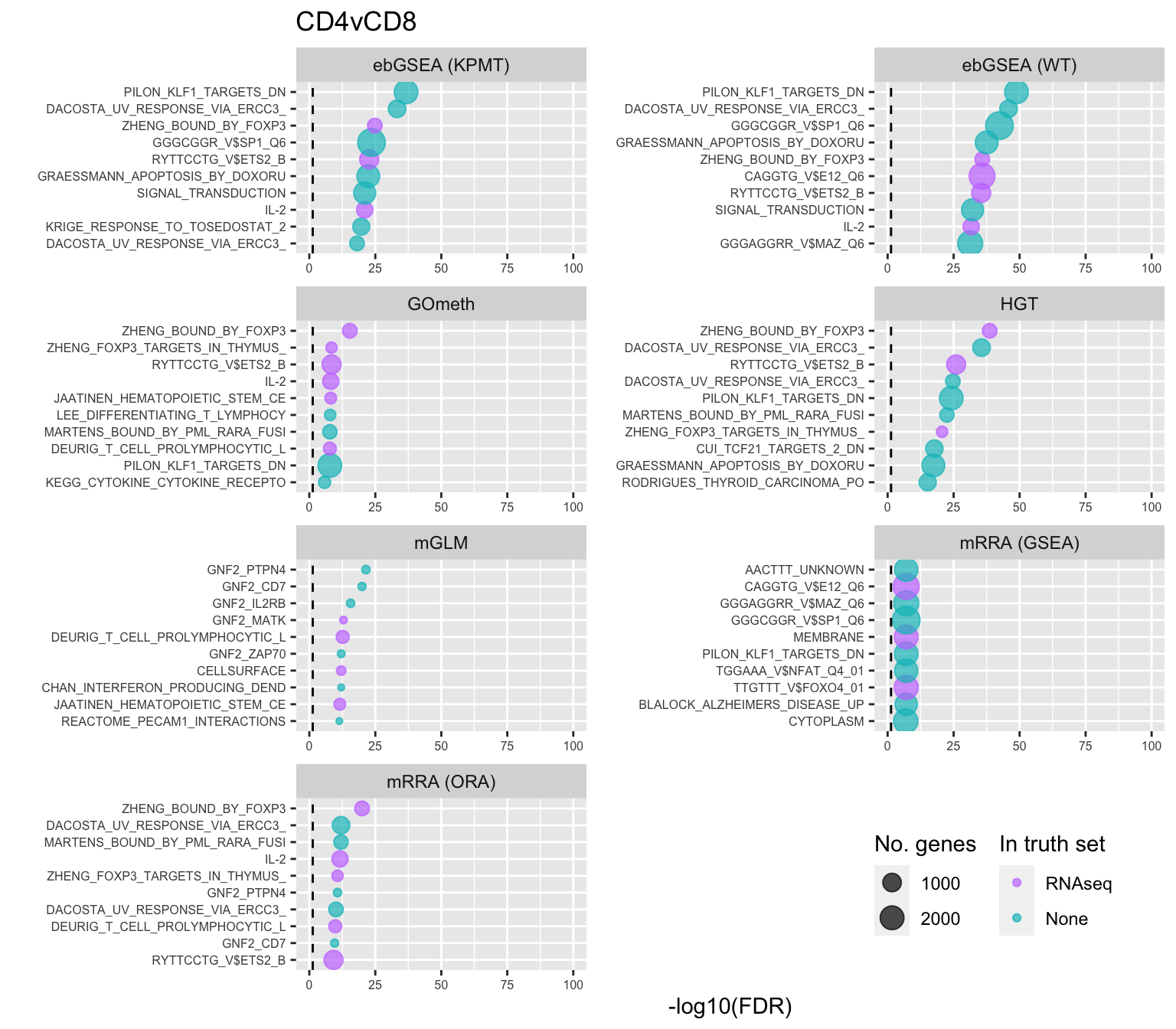
| Version | Author | Date |
|---|---|---|
| 4c57176 | JovMaksimovic | 2021-04-13 |
shift_legend(p[[3]], plot = TRUE, pos = "left")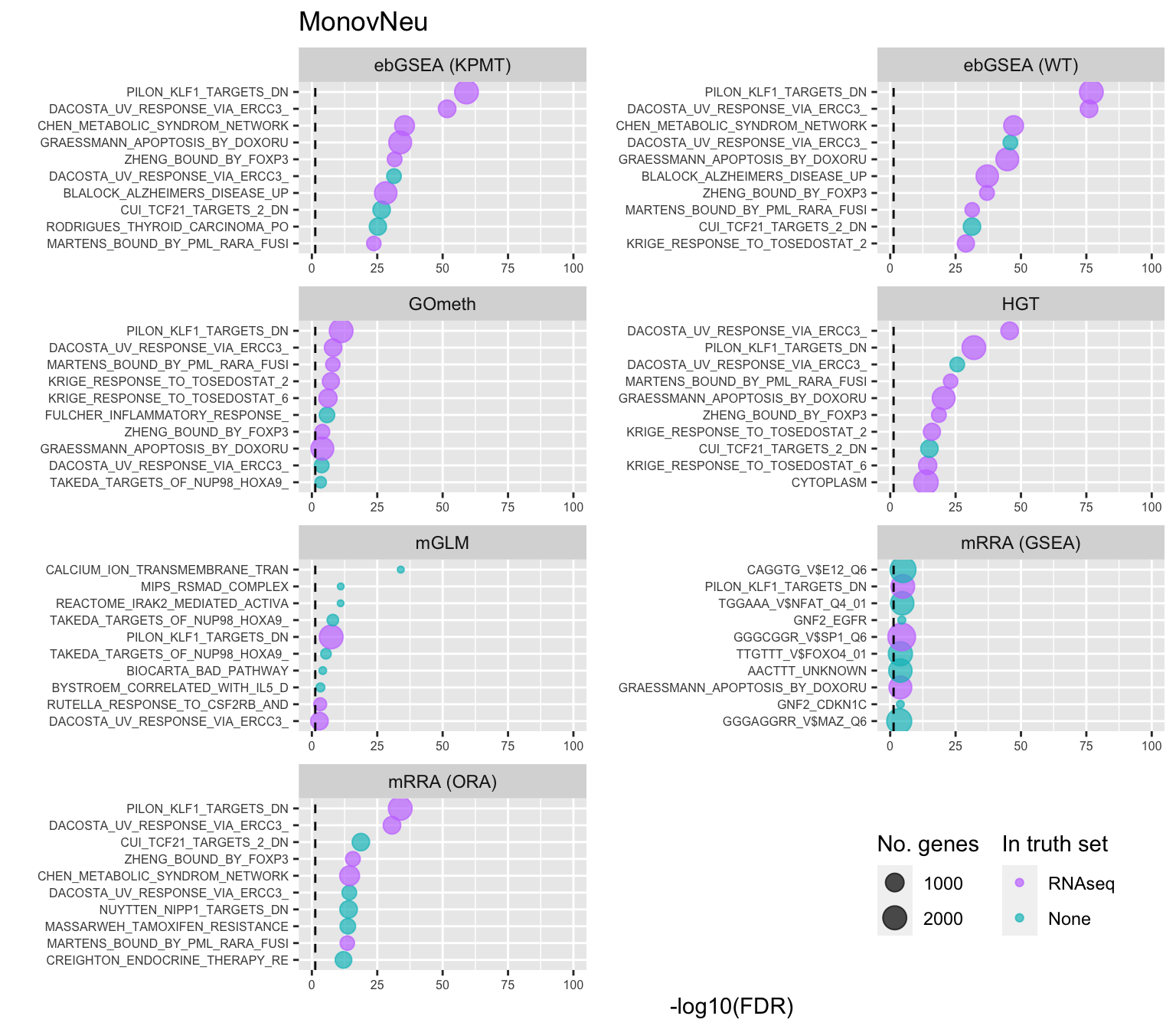
| Version | Author | Date |
|---|---|---|
| 4c57176 | JovMaksimovic | 2021-04-13 |
P-value histograms for the different methods for all contrasts on BROAD gene sets.
dat %>% filter(set == "BROAD") %>%
    filter(sub %in% c("n","c1")) %>%
    mutate(method = unname(dict[method])) -> subDat

ggplot(subDat, aes(pvalue, fill = method)) +
    geom_histogram(binwidth = 0.025) +
    facet_grid(cols = vars(contrast), rows = vars(method)) +
    theme(legend.position = "bottom") +
    labs(x = "P-value", y = "Frequency", fill = "Method") +
    scale_fill_manual(values = methodCols)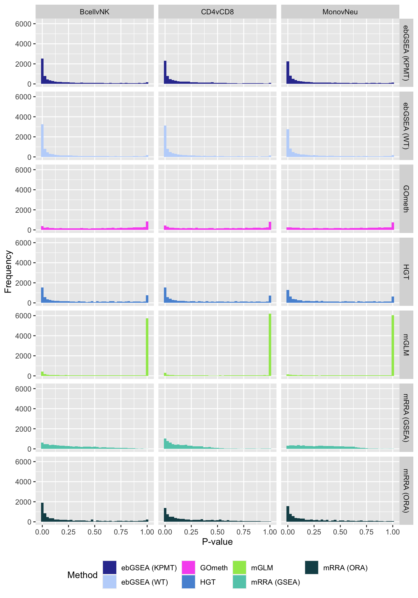
| Version | Author | Date |
|---|---|---|
| 4c57176 | JovMaksimovic | 2021-04-13 |
Compare GOmeth results using different DM CpG significance cutoffs
As the results of GOmeth depend on the list of significant CpGs provided as input to the function, we explored the effect of selecting "significant" CpGs in different ways on the gene set testing performance of GOmeth.
dat %>% filter(set == "BROAD") %>%
    filter(grepl("mmethyl", method)) %>%
    mutate(method = unname(dict[method])) %>%
    arrange(contrast, method, pvalue) %>%
    group_by(contrast, method, sub) %>%
    mutate(csum = cumsum(ID %in% topBROAD$ID)) %>%
    mutate(rank = 1:n()) %>%
    mutate(cut = ifelse(sub == "c1", "Top 5000",
                        ifelse(sub == "c2", "Top 10000",
                               ifelse(sub == "p1", "FDR < 0.01", "FDR < 0.05")))) %>%
    filter(rank <= 100) -> sub

p <- ggplot(sub, aes(x = rank, y = csum, colour = cut)) +
    geom_line() +
    facet_wrap(vars(contrast, method), ncol=2, nrow = 3, scales = "free") +
    geom_vline(xintercept = 10, linetype = "dotted") +
    labs(colour = "Sig. select", x = "Rank", y = "Cumulative no. immune sets") +
    theme(legend.position = "bottom")
p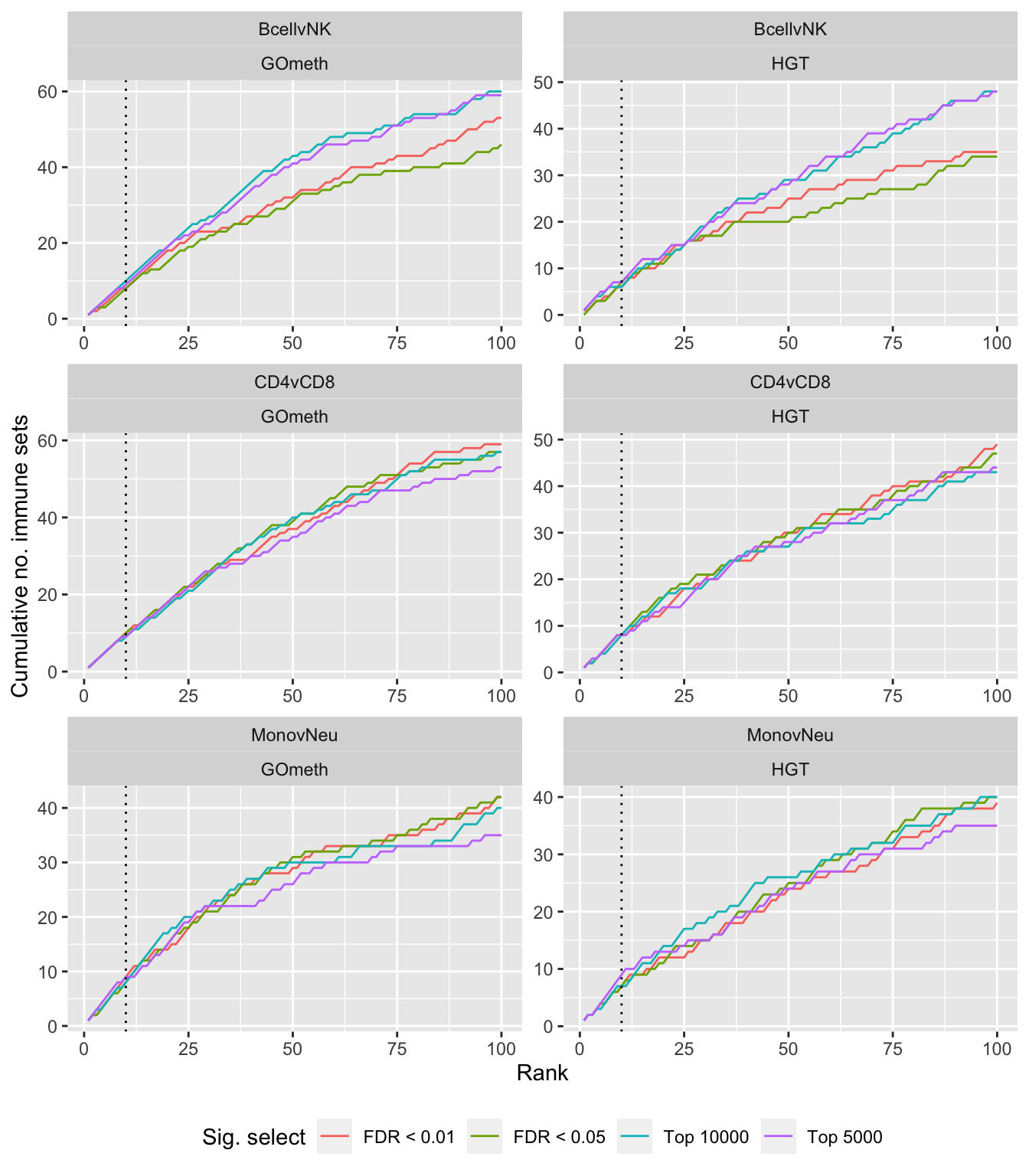
| Version | Author | Date |
|---|---|---|
| 4c57176 | JovMaksimovic | 2021-04-13 |
sessionInfo()R version 4.0.3 (2020-10-10)
Platform: x86_64-apple-darwin17.0 (64-bit)
Running under: macOS Mojave 10.14.6
Matrix products: default
BLAS: /Library/Frameworks/R.framework/Versions/4.0/Resources/lib/libRblas.dylib
LAPACK: /Library/Frameworks/R.framework/Versions/4.0/Resources/lib/libRlapack.dylib
locale:
[1] en_AU.UTF-8/en_AU.UTF-8/en_AU.UTF-8/C/en_AU.UTF-8/en_AU.UTF-8
attached base packages:
[1] grid stats4 parallel stats graphics grDevices utils
[8] datasets methods base
other attached packages:
[1] lemon_0.4.5
[2] ChAMPdata_2.22.0
[3] patchwork_1.1.1
[4] rbin_0.2.0
[5] forcats_0.5.1
[6] stringr_1.4.0
[7] dplyr_1.0.5
[8] purrr_0.3.4
[9] readr_1.4.0
[10] tidyr_1.1.3
[11] tibble_3.1.0
[12] tidyverse_1.3.0
[13] glue_1.4.2
[14] ggplot2_3.3.3
[15] missMethyl_1.24.0
[16] IlluminaHumanMethylationEPICanno.ilm10b4.hg19_0.6.0
[17] IlluminaHumanMethylation450kanno.ilmn12.hg19_0.6.0
[18] gridExtra_2.3
[19] reshape2_1.4.4
[20] BiocParallel_1.24.1
[21] limma_3.46.0
[22] paletteer_1.3.0
[23] minfi_1.36.0
[24] bumphunter_1.32.0
[25] locfit_1.5-9.4
[26] iterators_1.0.13
[27] foreach_1.5.1
[28] Biostrings_2.58.0
[29] XVector_0.30.0
[30] SummarizedExperiment_1.20.0
[31] Biobase_2.50.0
[32] MatrixGenerics_1.2.1
[33] matrixStats_0.58.0
[34] GenomicRanges_1.42.0
[35] GenomeInfoDb_1.26.7
[36] IRanges_2.24.1
[37] S4Vectors_0.28.1
[38] BiocGenerics_0.36.0
[39] here_1.0.1
[40] workflowr_1.6.2
loaded via a namespace (and not attached):
[1] readxl_1.3.1 backports_1.2.1
[3] BiocFileCache_1.14.0 plyr_1.8.6
[5] splines_4.0.3 digest_0.6.27
[7] htmltools_0.5.1.1 GO.db_3.12.1
[9] fansi_0.4.2 magrittr_2.0.1
[11] memoise_2.0.0 annotate_1.68.0
[13] modelr_0.1.8 askpass_1.1
[15] siggenes_1.64.0 prettyunits_1.1.1
[17] colorspace_2.0-0 rvest_1.0.0
[19] blob_1.2.1 rappdirs_0.3.3
[21] haven_2.3.1 xfun_0.22
[23] crayon_1.4.1 RCurl_1.98-1.3
[25] jsonlite_1.7.2 genefilter_1.72.1
[27] GEOquery_2.58.0 survival_3.2-10
[29] gtable_0.3.0 zlibbioc_1.36.0
[31] DelayedArray_0.16.3 Rhdf5lib_1.12.1
[33] HDF5Array_1.18.1 scales_1.1.1
[35] DBI_1.1.1 rngtools_1.5
[37] Rcpp_1.0.6 xtable_1.8-4
[39] progress_1.2.2 bit_4.0.4
[41] mclust_5.4.7 preprocessCore_1.52.1
[43] httr_1.4.2 RColorBrewer_1.1-2
[45] ellipsis_0.3.1 farver_2.1.0
[47] pkgconfig_2.0.3 reshape_0.8.8
[49] XML_3.99-0.6 sass_0.3.1
[51] dbplyr_2.1.1 utf8_1.2.1
[53] labeling_0.4.2 tidyselect_1.1.0
[55] rlang_0.4.10 later_1.1.0.1
[57] AnnotationDbi_1.52.0 cellranger_1.1.0
[59] munsell_0.5.0 tools_4.0.3
[61] cachem_1.0.4 cli_2.4.0
[63] generics_0.1.0 RSQLite_2.2.5
[65] broom_0.7.6 evaluate_0.14
[67] fastmap_1.1.0 yaml_2.2.1
[69] rematch2_2.1.2 org.Hs.eg.db_3.12.0
[71] knitr_1.31 bit64_4.0.5
[73] fs_1.5.0 beanplot_1.2
[75] scrime_1.3.5 nlme_3.1-152
[77] doRNG_1.8.2 sparseMatrixStats_1.2.1
[79] whisker_0.4 nor1mix_1.3-0
[81] xml2_1.3.2 biomaRt_2.46.3
[83] rstudioapi_0.13 compiler_4.0.3
[85] curl_4.3 reprex_2.0.0
[87] statmod_1.4.35 bslib_0.2.4
[89] stringi_1.5.3 highr_0.8
[91] GenomicFeatures_1.42.3 lattice_0.20-41
[93] Matrix_1.3-2 multtest_2.46.0
[95] vctrs_0.3.7 pillar_1.5.1
[97] lifecycle_1.0.0 rhdf5filters_1.2.0
[99] jquerylib_0.1.3 cowplot_1.1.1
[101] data.table_1.14.0 bitops_1.0-6
[103] httpuv_1.5.5 rtracklayer_1.50.0
[105] R6_2.5.0 promises_1.2.0.1
[107] codetools_0.2-18 MASS_7.3-53.1
[109] assertthat_0.2.1 rhdf5_2.34.0
[111] openssl_1.4.3 rprojroot_2.0.2
[113] withr_2.4.1 GenomicAlignments_1.26.0
[115] Rsamtools_2.6.0 GenomeInfoDbData_1.2.4
[117] mgcv_1.8-34 hms_1.0.0
[119] quadprog_1.5-8 base64_2.0
[121] rmarkdown_2.7 DelayedMatrixStats_1.12.3
[123] illuminaio_0.32.0 git2r_0.28.0
[125] lubridate_1.7.10