B-ALL Experiment 1: BoneMarrowMap Annotation
Symphony reference projection, cell type label transfer, and Figure 3D
Jovana Maksimovic
July 15, 2026
Last updated: 2026-07-15
Checks: 7 0
Knit directory: flex-fusion-probes/
This reproducible R Markdown analysis was created with workflowr (version 1.7.1). The Checks tab describes the reproducibility checks that were applied when the results were created. The Past versions tab lists the development history.
Great! Since the R Markdown file has been committed to the Git repository, you know the exact version of the code that produced these results.
Great job! The global environment was empty. Objects defined in the global environment can affect the analysis in your R Markdown file in unknown ways. For reproduciblity it’s best to always run the code in an empty environment.
The command set.seed(20240925) was run prior to running
the code in the R Markdown file. Setting a seed ensures that any results
that rely on randomness, e.g. subsampling or permutations, are
reproducible.
Great job! Recording the operating system, R version, and package versions is critical for reproducibility.
Nice! There were no cached chunks for this analysis, so you can be confident that you successfully produced the results during this run.
Great job! Using relative paths to the files within your workflowr project makes it easier to run your code on other machines.
Great! You are using Git for version control. Tracking code development and connecting the code version to the results is critical for reproducibility.
The results in this page were generated with repository version de6e8c4. See the Past versions tab to see a history of the changes made to the R Markdown and HTML files.
Note that you need to be careful to ensure that all relevant files for
the analysis have been committed to Git prior to generating the results
(you can use wflow_publish or
wflow_git_commit). workflowr only checks the R Markdown
file, but you know if there are other scripts or data files that it
depends on. Below is the status of the Git repository when the results
were generated:
Ignored files:
    Ignored:    .DS_Store
    Ignored:    .Rhistory
    Ignored:    .Rproj.user/
    Ignored:    analysis/.gitignore
    Ignored:    analysis/TOM/
    Ignored:    analysis/obsolete/B-ALL_nonblast_fusion_analysis_cache/
    Ignored:    analysis/projectionFigures/
    Ignored:    code/files/
    Ignored:    data/.DS_Store
    Ignored:    data/BoneMarrowMap/
    Ignored:    data/BoneMarrowMapBoneMarrowMap_SymphonyReference.rds
    Ignored:    data/BoneMarrowMapBoneMarrowMap_uwot_model.uwot
    Ignored:    data/CAPTURE-1-POOL-FLEX/
    Ignored:    data/CAPTURE-2-POOL-FLEX/
    Ignored:    data/Pool-240917-FLEX/
    Ignored:    data/RDS/
    Ignored:    data/Run_1_and_Run_2/
    Ignored:    data/Run_2/
    Ignored:    logs/
    Ignored:    output/
    Ignored:    renv/library/
    Ignored:    renv/staging/

Untracked files:
    Untracked:  CLAUDE.md
    Untracked:  analysis/B-ALL_exp2_c1437_clone_analysis.Rmd
    Untracked:  analysis/B-ALL_exp2_c369_mrd_analysis.Rmd
    Untracked:  analysis/B-ALL_exp2_joint_clustering.Rmd
    Untracked:  analysis/fig4_assembly.Rmd
    Untracked:  data/sample_information_flex_experiment_2_table.csv
    Untracked:  poster.pptx

Unstaged changes:
    Modified:   analysis/B-ALL_exp2_annotate_with_BoneMarrowMap.Rmd
    Deleted:    analysis/B-ALL_exp2_c1437_li2025_clone_analysis.Rmd
    Modified:   analysis/B-ALL_exp2_quality_control.Rmd
    Modified:   analysis/B-ALL_nonblast_fusion_analysis.Rmd
    Modified:   analysis/index.Rmd
    Modified:   render_all.sh
Note that any generated files, e.g. HTML, png, CSS, etc., are not included in this status report because it is ok for generated content to have uncommitted changes.
These are the previous versions of the repository in which changes were
made to the R Markdown
(analysis/B-ALL_exp1_annotate_with_BoneMarrowMap.Rmd) and
HTML (docs/B-ALL_exp1_annotate_with_BoneMarrowMap.html)
files. If you’ve configured a remote Git repository (see
?wflow_git_remote), click on the hyperlinks in the table
below to view the files as they were in that past version.
| File | Version | Author | Date | Message |
|---|---|---|---|---|
| Rmd | de6e8c4 | Jovana Maksimovic | 2026-07-15 | wflow_publish("analysis/B-ALL_exp1_annotate_with_BoneMarrowMap.Rmd") |
| html | bb2d2c8 | Jovana Maksimovic | 2026-05-14 | Build site. |
| Rmd | 6f855be | Jovana Maksimovic | 2026-05-14 | Filter all exp1 doublets regardless of fusion status |
| html | 1b5bb97 | Jovana Maksimovic | 2026-05-11 | Build site. |
| Rmd | 1f3159b | Jovana Maksimovic | 2026-05-08 | Rename RDS checkpoints to systematic naming scheme |
| Rmd | 71c5f99 | Jovana Maksimovic | 2026-05-08 | docs: add getting_started page; fix myeloid_types error; move exploratory notebooks to obsolete |
| Rmd | 1578018 | Jovana Maksimovic | 2026-05-08 | docs: add prose, standardise headings and figure labels across all 10 B-ALL notebooks |
| Rmd | 1a33400 | Jovana Maksimovic | 2026-05-08 | B-ALL cleanup: fix index links, stray library() calls, add chunk labels |
| Rmd | 1724beb | Jovana Maksimovic | 2026-05-08 | Standardise YAML headers and chunk names across all notebooks; merge utility_functions into utilities.R |
| Rmd | 10d2f5e | Jovana Maksimovic | 2026-05-08 | Rename analysis notebooks to new naming scheme |
This notebook projects B-ALL Experiment 1 cells onto the BoneMarrowMap haematopoietic reference using Symphony (Kang et al., 2021), transfers broad and fine-grained cell type labels, and computes haematopoietic pseudotime estimates. The three patient samples (MLM_22_DX, EKL44_2_DX, EKL44_2_Rel) are analysed together after excluding the MCF7 control cells.
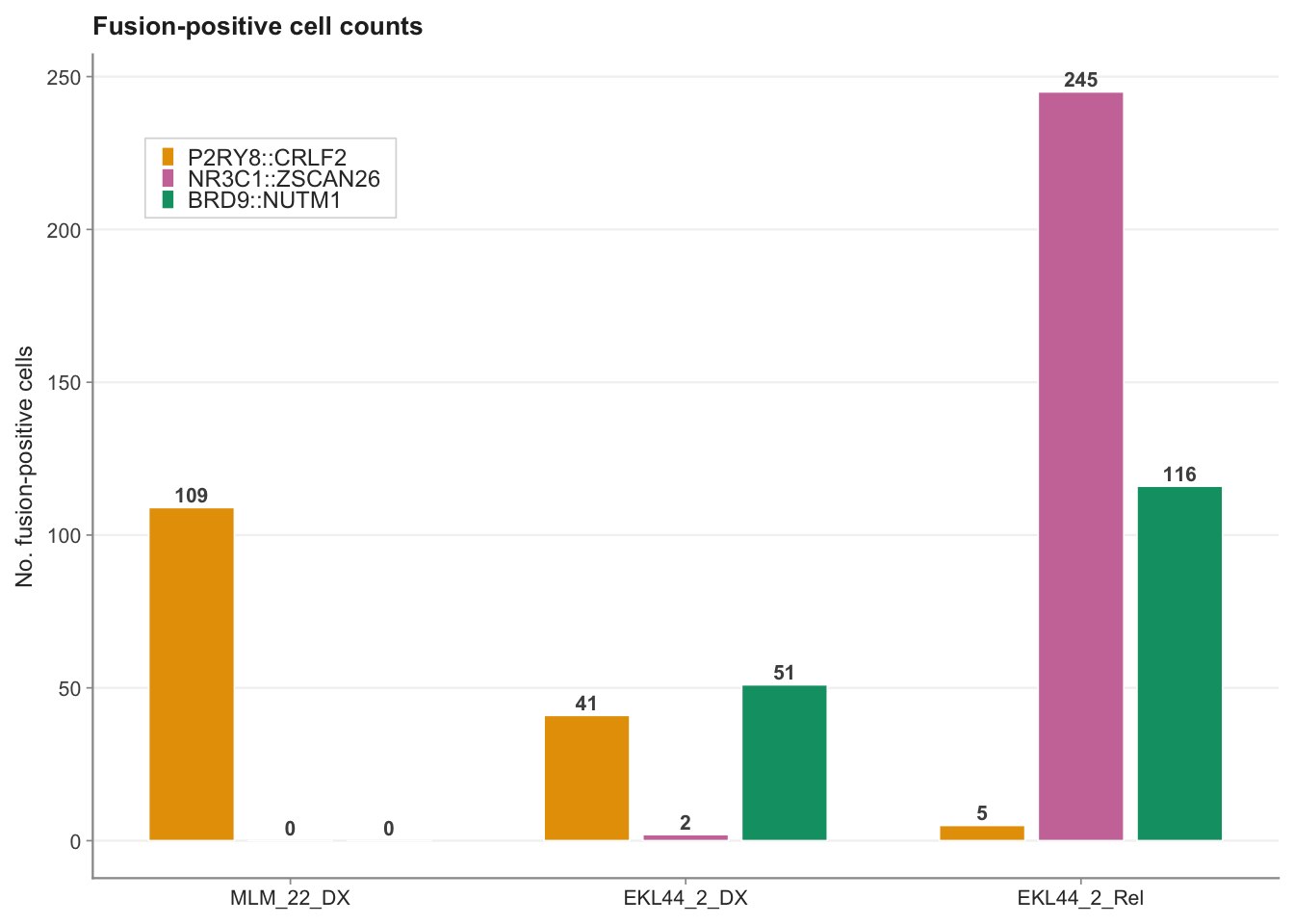
This notebook contributes to Figure 3D
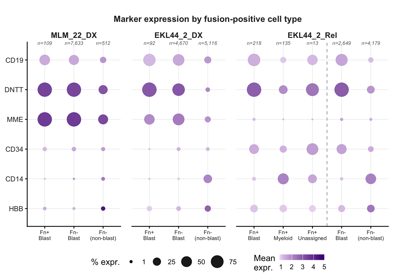
(fusion-positive cell counts bar chart) in the paper. It also contains
an EKL44_2-only fusion/lineage dot plot (below) that was previously
labelled Supplementary Figure 3A; that panel has since
been dropped as redundant with panel C of Supplementary Figure
2 (B-ALL_exp1_clustering.Rmd), which shows marker
expression per cell type for all three samples including both EKL44_2
timepoints. The chunk is kept here for reference but is no longer part
of any figure.
Load data
file <- here("data", "RDS", "exp1_qc.sce.rds")
sce <- readRDS(file)
Convert Ensembl IDs to gene symbols, appending the Ensembl ID to resolve any duplicate symbol names. MCF7 cells are then excluded to create a B-ALL-only Seurat object.
# change gene IDs to Symbols before creating Seurat object
rownames(sce) <- rowData(sce)$Symbol
dups <- rownames(sce)[duplicated(rownames(sce))]
rownames(sce) <- ifelse(rownames(sce) %in% dups,
                        paste0(rownames(sce),"_",rowData(sce)$ID),
                        rownames(sce))
table(duplicated(rownames(sce)))
FALSE
37170
seu <- CreateSeuratObject(counts = counts(sce)[, sce$Sample != "MCF7"],
meta.data = colData(sce[, sce$Sample != "MCF7"]) %>% data.frame)
seu$Sample <- fct_drop(seu$Sample)
seuAn object of class Seurat
37170 features across 25328 samples within 1 assay
Active assay: RNA (37170 features, 0 variable features)
1 layer present: countsseu$fusion_detected <- colSums(seu[["RNA"]]$counts[grepl("fusion", rownames(seu)),]) > 0
VlnPlot(seu, features = "sum", group.by = "fusion_detected",
pt.size = 0, log = TRUE)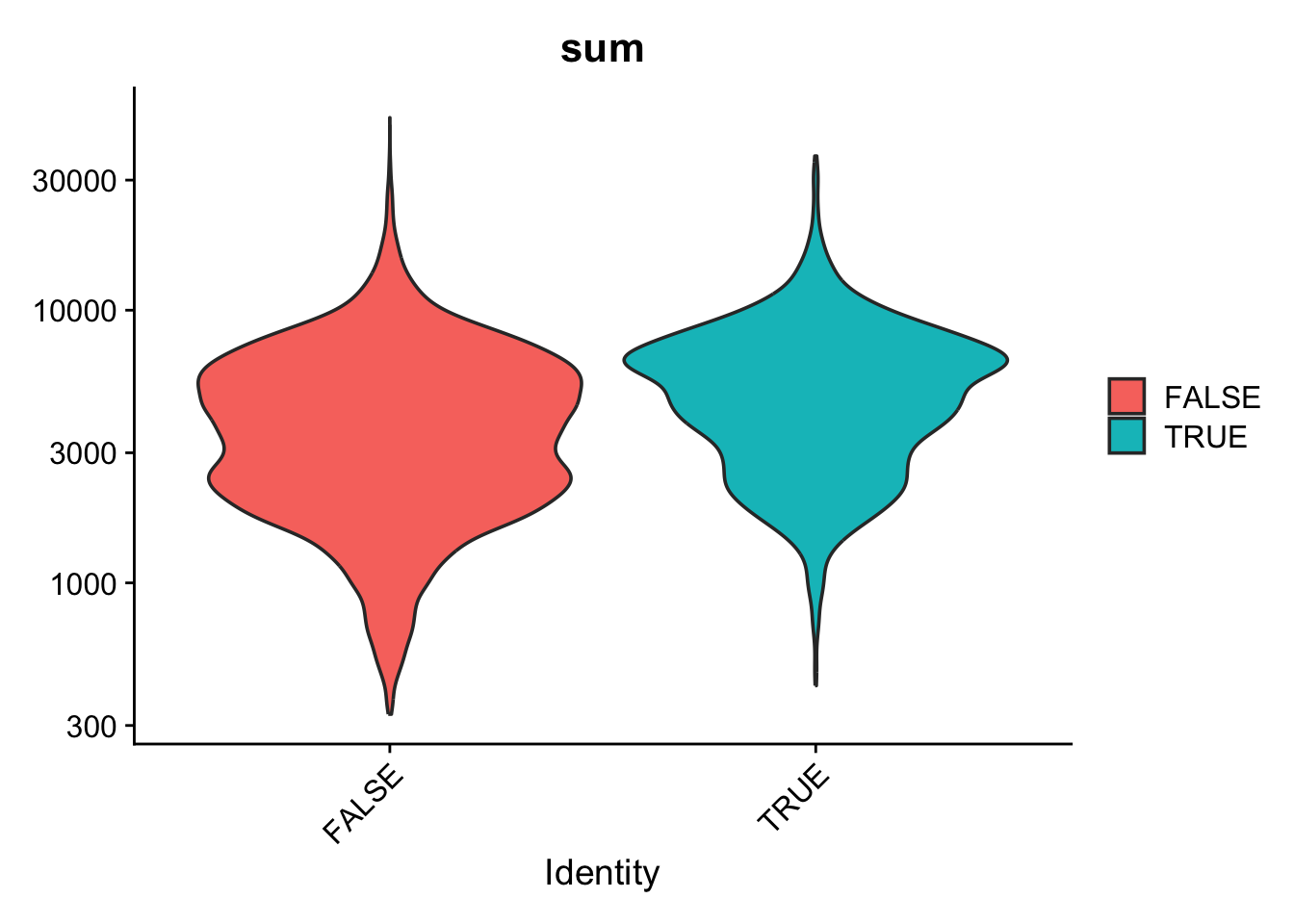
| Version | Author | Date |
|---|---|---|
| 1b5bb97 | Jovana Maksimovic | 2026-05-11 |
seu@meta.data %>%
  dplyr::select(sum, fusion_detected) %>%
  ggplot(aes(x = fusion_detected, y = sum)) +
  geom_boxplot() +
  scale_y_log10()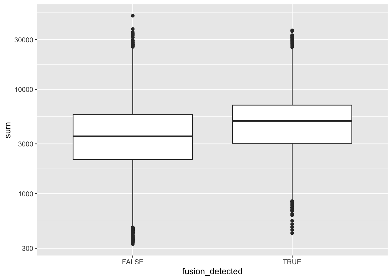
| Version | Author | Date |
|---|---|---|
| 1b5bb97 | Jovana Maksimovic | 2026-05-11 |
Fusion transcript detection
Label fusion-expressing cells.
patient_fusions <- c("P2RY8-CRLF2-fusion", "BRD9-NUTM1-fusion", "NR3C1-ZSCAN26-fusion")
patient_fusions_detected <- colSums(seu[["RNA"]]$counts[rownames(seu) %in% patient_fusions,]) > 0

table(patient_fusions_detected)
patient_fusions_detected
FALSE TRUE
24759 569 fusion_type <- ifelse(seu[["RNA"]]$counts[rownames(seu) == "P2RY8-CRLF2-fusion", ] > 0,
"P2RY8-CRLF2-fusion",
ifelse(seu[["RNA"]]$counts[rownames(seu) == "BRD9-NUTM1-fusion", ] > 0,
"BRD9-NUTM1-fusion",
ifelse(seu[["RNA"]]$counts[rownames(seu) == "NR3C1-ZSCAN26-fusion", ] > 0,
"NR3C1-ZSCAN26-fusion", "not-detected")))
seu$patient_fusion <- fusion_type
table(seu$patient_fusion, seu$Sample)
                       EKL44_2_DX EKL44_2_Rel MLM_22_DX
  BRD9-NUTM1-fusion            51         116         0
  not-detected               9786        6828      8145
  NR3C1-ZSCAN26-fusion          2         245         0
  P2RY8-CRLF2-fusion           41           5       109
All doublets are removed regardless of fusion status. A doublet carrying fusion UMI most likely represents a blast paired with a non-blast cell; retaining it would inflate library size, distort cell type proportions, and introduce a mixed transcriptome into downstream analysis.
# Report how many fusion-positive cells are classified as doublets before removal
seu@meta.data %>%
  group_by(scDblFinder.class, patient_fusion) %>%
  summarise(n = n(), .groups = "drop") %>%
  tidyr::pivot_wider(names_from = scDblFinder.class, values_from = n, values_fill = 0) %>%
knitr::kable(caption = "Cell counts by doublet class and fusion status before doublet removal.")| patient_fusion | singlet |
|---|---|
| BRD9-NUTM1-fusion | 167 |
| NR3C1-ZSCAN26-fusion | 247 |
| P2RY8-CRLF2-fusion | 155 |
| not-detected | 24759 |
VlnPlot(seu, features = "sum", group.by = "patient_fusion",
        pt.size = 0, log = TRUE)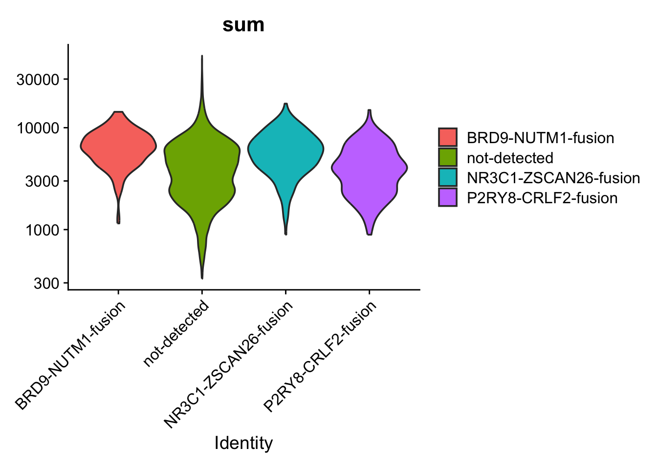
seu$fusion_detected <- seu$patient_fusion != "not-detected"
VlnPlot(seu, features = "sum", group.by = "fusion_detected",
        pt.size = 0, log = TRUE)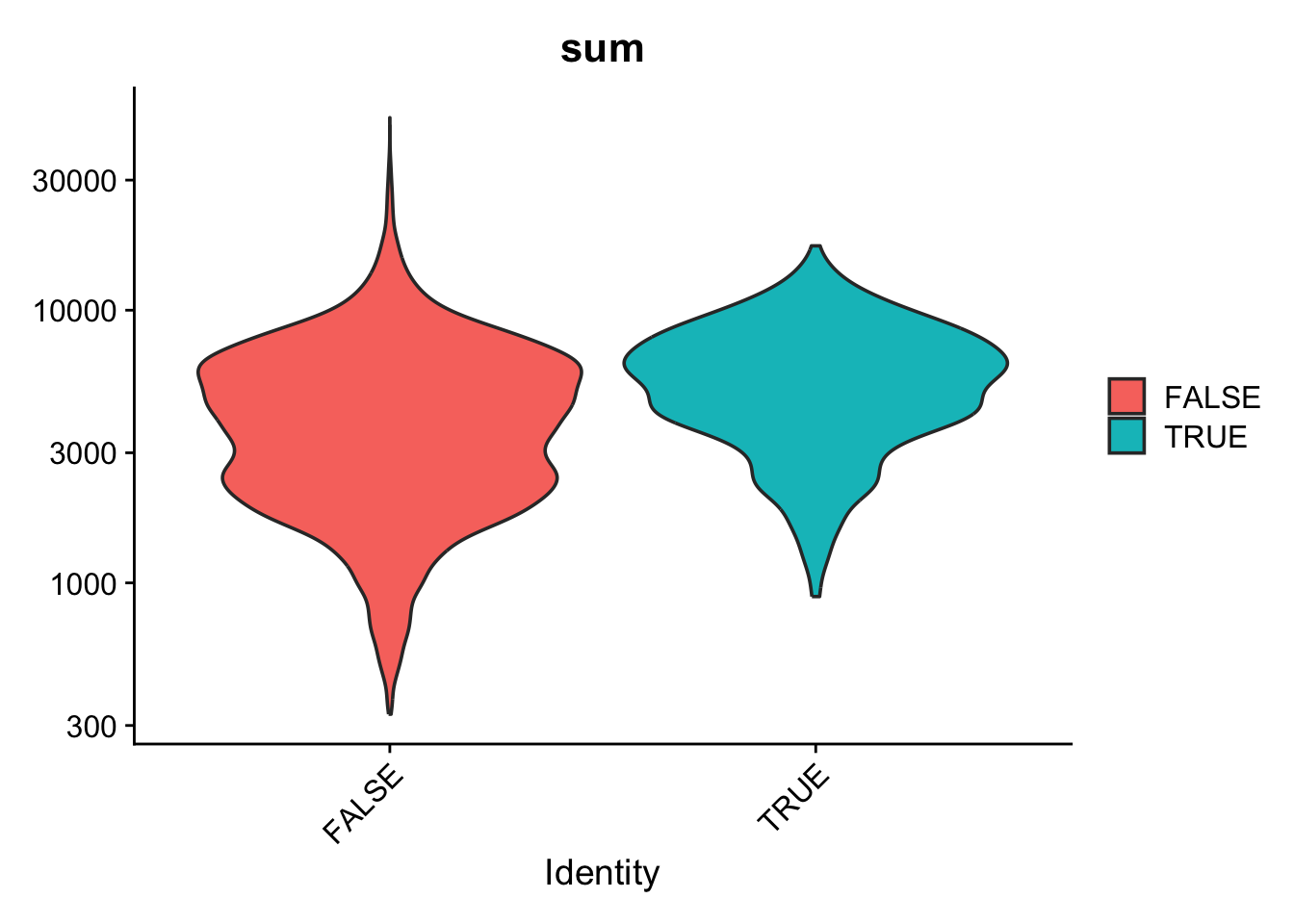
BoneMarrowMap reference
Download the BoneMarrowMap Symphony reference object and pre-trained
UMAP model if not already cached locally. Files are stored in
data/BoneMarrowMap/ (≈565 Mb total).
projection_path = here("data/BoneMarrowMap")
# Set directory to store projection reference files
if(!dir.exists(projection_path)) dir.create(projection_path)

# Download Bone Marrow Reference - 344 Mb
rds <- paste0(projection_path, 'BoneMarrowMap_SymphonyReference.rds')
if(!file.exists(rds)){
  curl::curl_download('https://bonemarrowmap.s3.us-east-2.amazonaws.com/BoneMarrowMap_SymphonyReference.rds',
                      destfile = rds)
}

uwot <- paste0(projection_path, 'BoneMarrowMap_uwot_model.uwot')
if(!file.exists(uwot)){
  # Download uwot model file - 221 Mb
  curl::curl_download('https://bonemarrowmap.s3.us-east-2.amazonaws.com/BoneMarrowMap_uwot_model.uwot',
                      destfile = uwot)
}

# Load Symphony reference
ref <- readRDS(rds)
# Set uwot path for UMAP projection
ref$save_uwot_path <- uwot
Visualise BoneMarrowMap reference
Creating a lightweight Seurat object from the Symphony reference (coordinates and metadata only, no expression counts) to visualise the reference UMAP and confirm the expected structure before projecting query cells.
ReferenceSeuratObj <- create_ReferenceObject(ref)

DimPlot(ReferenceSeuratObj, reduction = 'umap', group.by = 'CellType_Annotation_formatted',
        raster=FALSE, label=TRUE, label.size = 2) + NoLegend()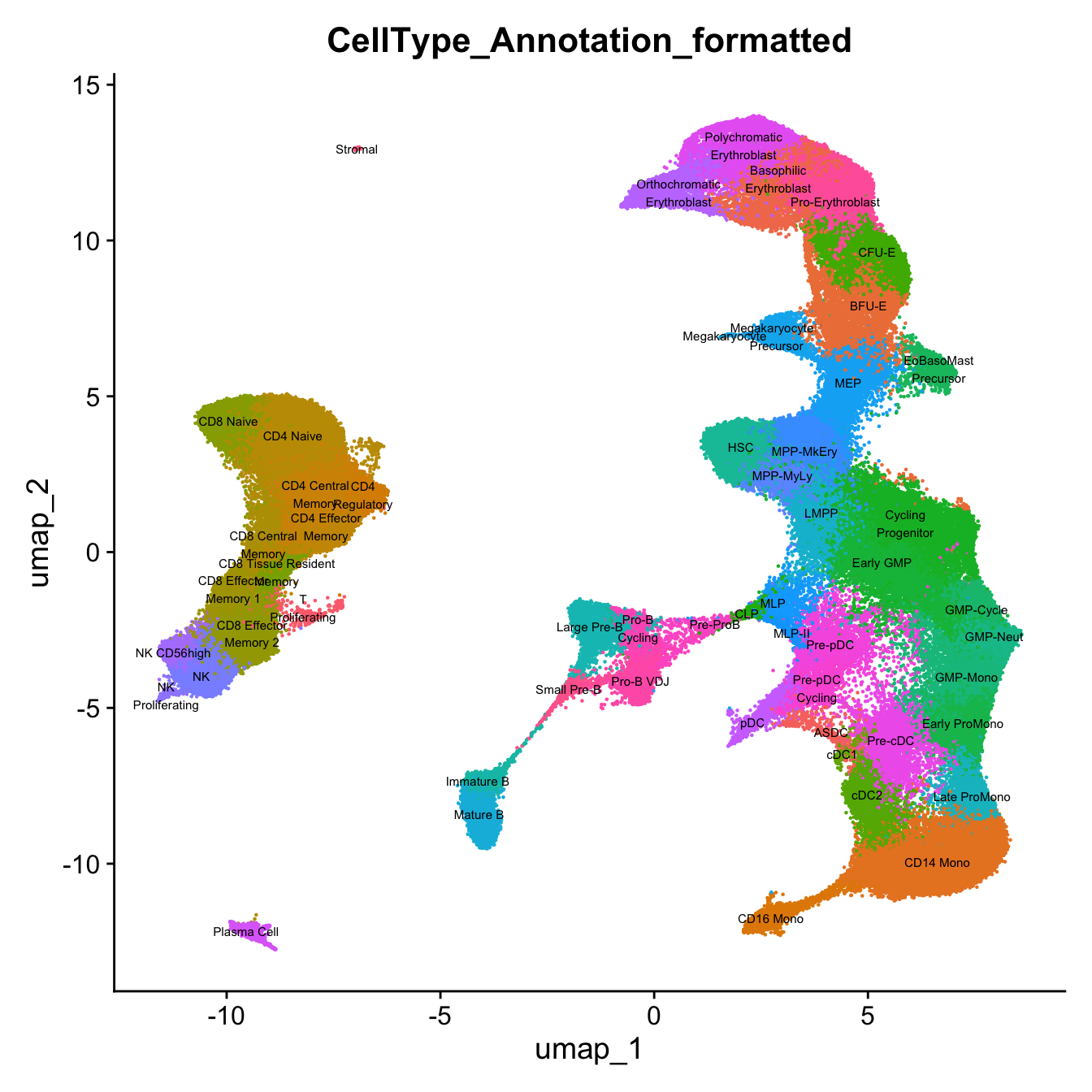
| Version | Author | Date |
|---|---|---|
| 1b5bb97 | Jovana Maksimovic | 2026-05-11 |
We can also visualize broader cell type labels which may simplify interpretation and downstream analysis.
DimPlot(ReferenceSeuratObj, reduction = 'umap', group.by = 'CellType_Broad',
        raster=FALSE, label=TRUE, label.size = 2) + NoLegend()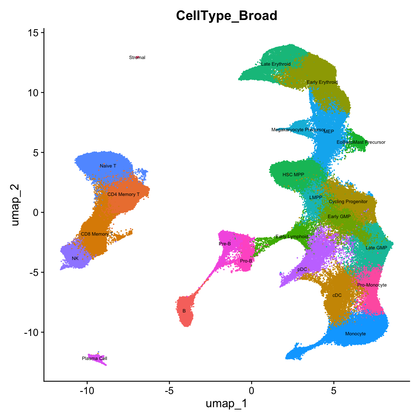
| Version | Author | Date |
|---|---|---|
| 1b5bb97 | Jovana Maksimovic | 2026-05-11 |
We can visualize other annotations too, including cell cycle phase and lineage pseudotime estimates.
p1 <- DimPlot(ReferenceSeuratObj, reduction = 'umap', group.by = 'CyclePhase', raster=FALSE)
p2 <- FeaturePlot(ReferenceSeuratObj, reduction = 'umap', features = 'Pseudotime', raster=FALSE)

p1 + p2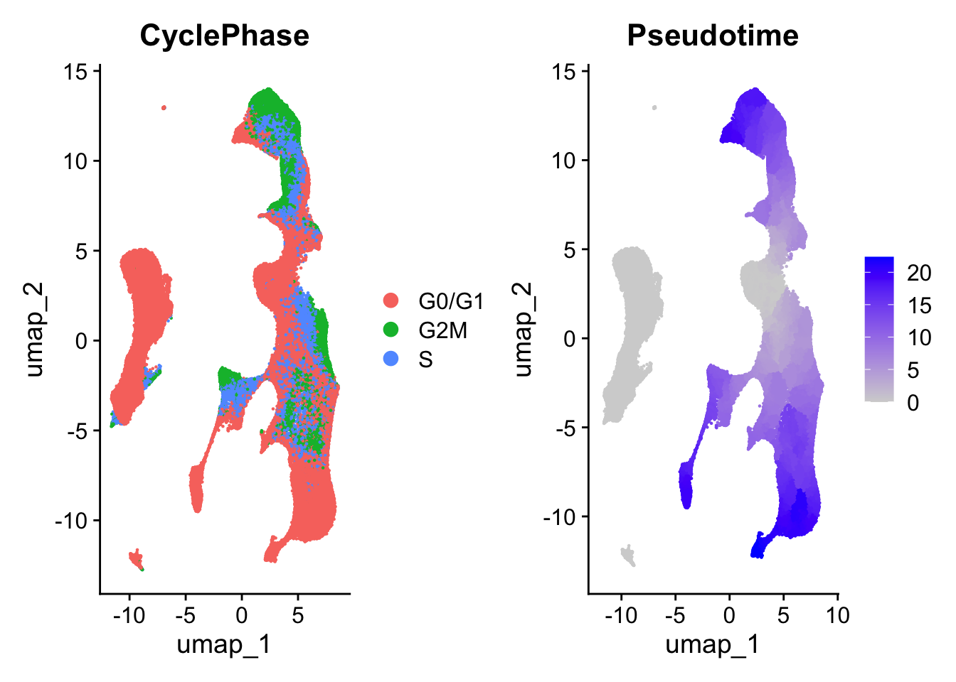
| Version | Author | Date |
|---|---|---|
| 1b5bb97 | Jovana Maksimovic | 2026-05-11 |
Project query onto the reference
Project the B-ALL query cells onto the BoneMarrowMap reference using
Symphony. Batch correction is applied per sample (Sample
key). The mapping error score is then used to flag low-quality
projections, with cells failing QC excluded from cell type assignment
(unless they carry a patient fusion).
query <- seu
# batch variable to correct in the query data, set as NULL if no batches in query
batchvar <- 'Sample'

# Map query dataset using Symphony (Kang et al 2021)
query <- map_Query(
    exp_query = query@assays$RNA$counts,
    metadata_query = query@meta.data,
    ref_obj = ref,
    vars = batchvar
)
In leukemia samples, the distribution of mapping error scores can vary broadly from sample to sample. In this context, we will want to threshold outliers with high mapping error on a per-sample basis. Typically, a threshold of 2, 2.5, or 3 MADs works well.
In some cases where sequencing depth is very low (e.g. older datasets from first-generation scRNA-seq protocols), a more stringent threshold of even 1.5 may be warranted to eliminate cells with low mapping quality
# Run QC based on mapping error score, flag cells with mapping error >= 2.5 MADs above median
query <- query %>%
  calculate_MappingError(., reference = ref, MAD_threshold = 3,
                         threshold_by_donor = TRUE,
                         donor_key = batchvar) # threshold mapping error on a per-sample basis.

# Plot distribution by patient to ensure you are catching the tail
query@meta.data %>%
  ggplot(aes(x = mapping_error_score, fill = mapping_error_QC)) +
  geom_histogram(bins = 200) + facet_wrap(.~get(batchvar))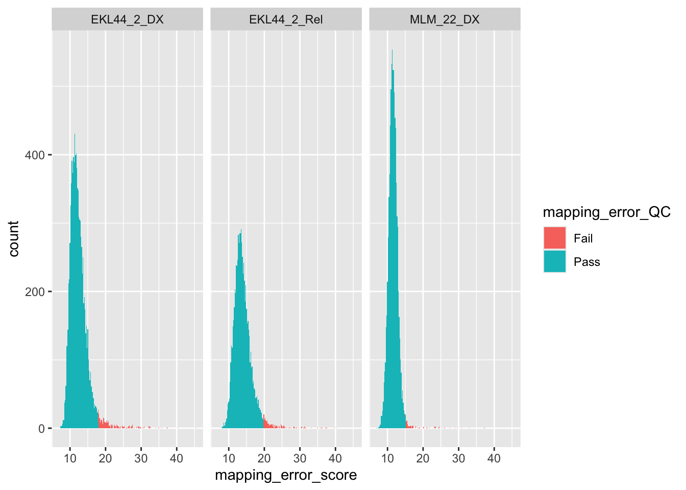
# Get QC Plots
QC_plots <- plot_MappingErrorQC(query)

# Plot together
patchwork::wrap_plots(QC_plots, ncol = 2)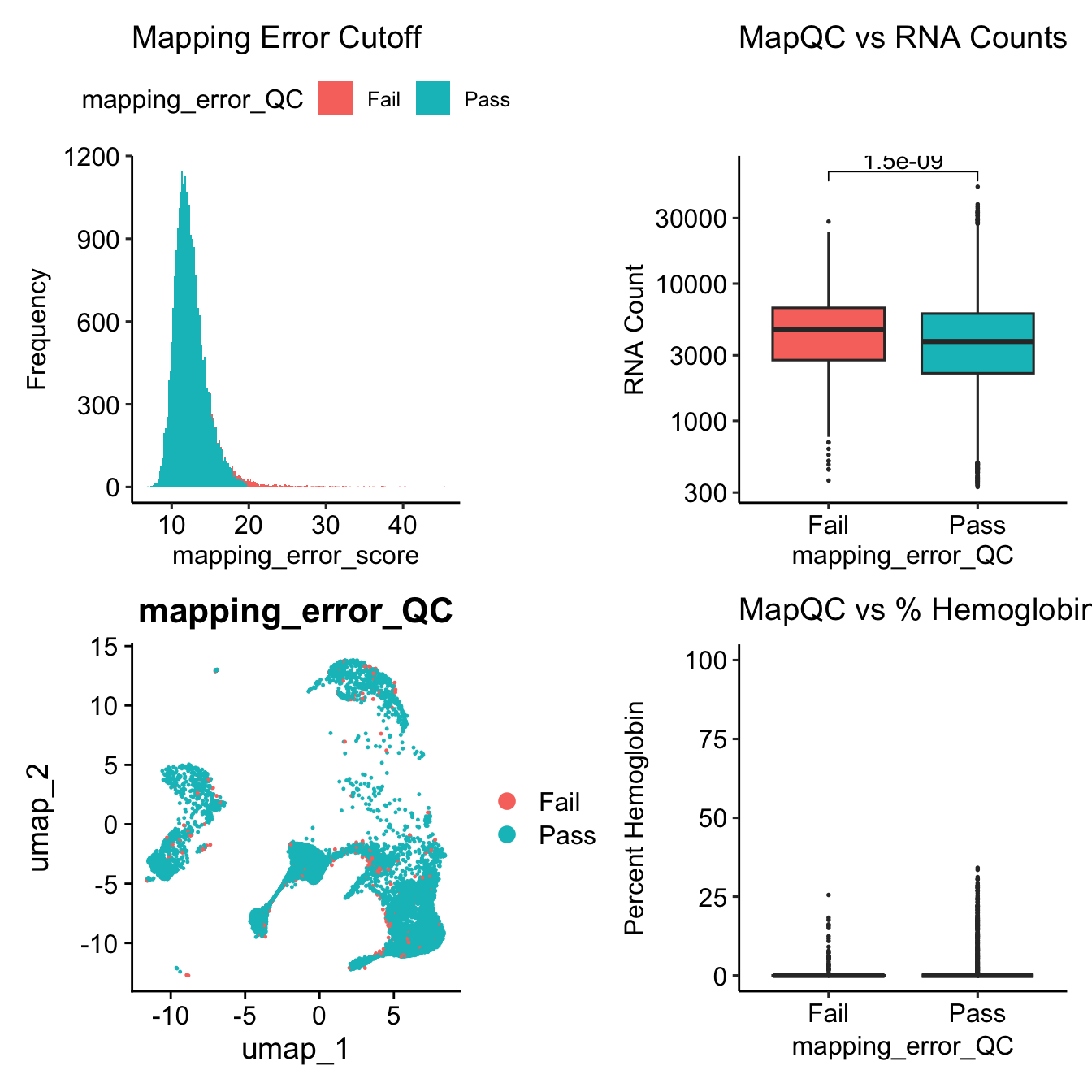
Cell type assignment
Cell identities are assigned by KNN classification (k = 30 nearest
neighbours) from the reference map, transferring both precise
(predicted_CellType) and broad
(predicted_CellType_Broad) labels. Cells that failed
mapping QC are excluded, with the exception of fusion-positive cells —
leukaemic blasts with a strongly aberrant transcriptome can legitimately
exceed the mapping error threshold on a normal haematopoiesis reference.
Broader cell type labels will also be transferred automatically along
with the precise cell type labels. This label transfer step should take
<1 min for 10,000 cells and <5 min for 100,000 cells.
#query <- subset(query, mapping_error_QC == 'Pass' | patient_fusion != "not-detected")

# Predict Hematopoietic Cell Types by KNN classification
query <- predict_CellTypes(
  query_obj = query,
  ref_obj = ref,
  initial_label = 'initial_CellType', # celltype assignments before filtering on mapping QC
  final_label = 'predicted_CellType'  # celltype assignments with map QC failing cells assigned as NA
)

DimPlot(query, reduction = 'umap_projected',
        group.by = c('predicted_CellType'),
        raster=FALSE, label=TRUE, label.size = 2) + NoLegend()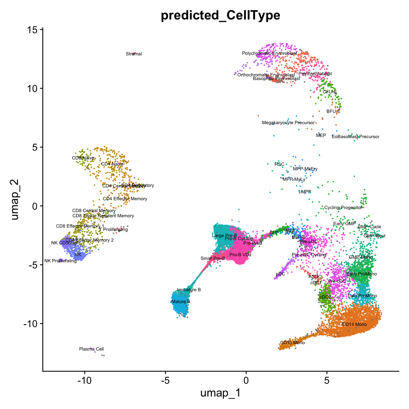
cells.highlight <- split(which(query$patient_fusion != "not-detected"),
                                query$patient_fusion[query$patient_fusion != "not-detected"])

DimPlot(query, reduction = 'umap_projected',
        group.by = c('predicted_CellType'),
        raster = FALSE,
        label = TRUE,
        label.size = 2.5,
        repel = T,
        cells.highlight = cells.highlight,
        cols.highlight = setNames(c("red","green","purple"),
                                  names(cells.highlight))) +
  theme(legend.position = "bottom") -> p1

p1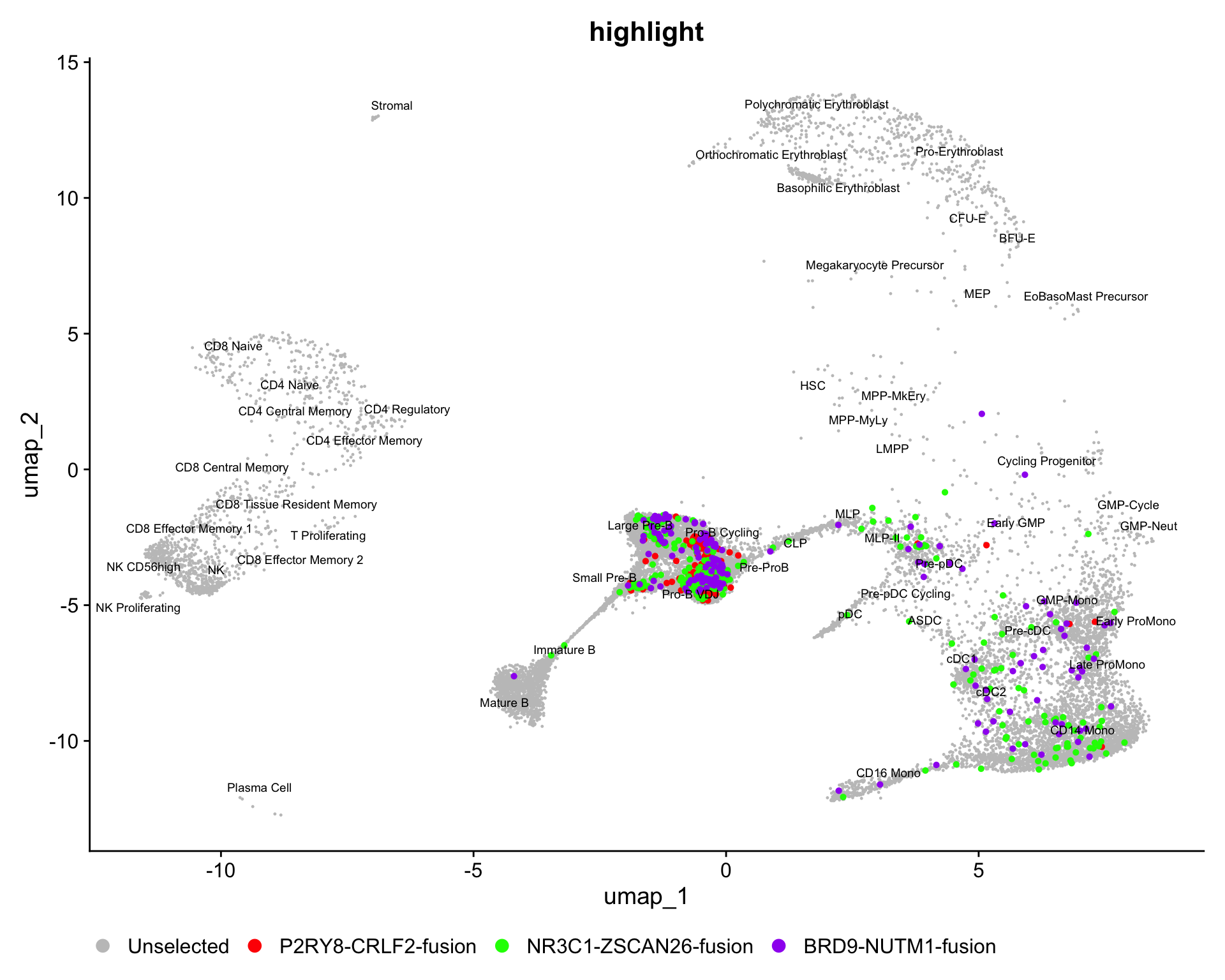
We can also visualize the broader cell type categories in case precise labels are too granular. These provide a simpler view of the data and can help guide cluster annotations if your dataset does not have many cells.
DimPlot(query, reduction = 'umap_projected',
        group.by = c('predicted_CellType_Broad'),
        raster=FALSE, label=TRUE, label.size = 3) + NoLegend()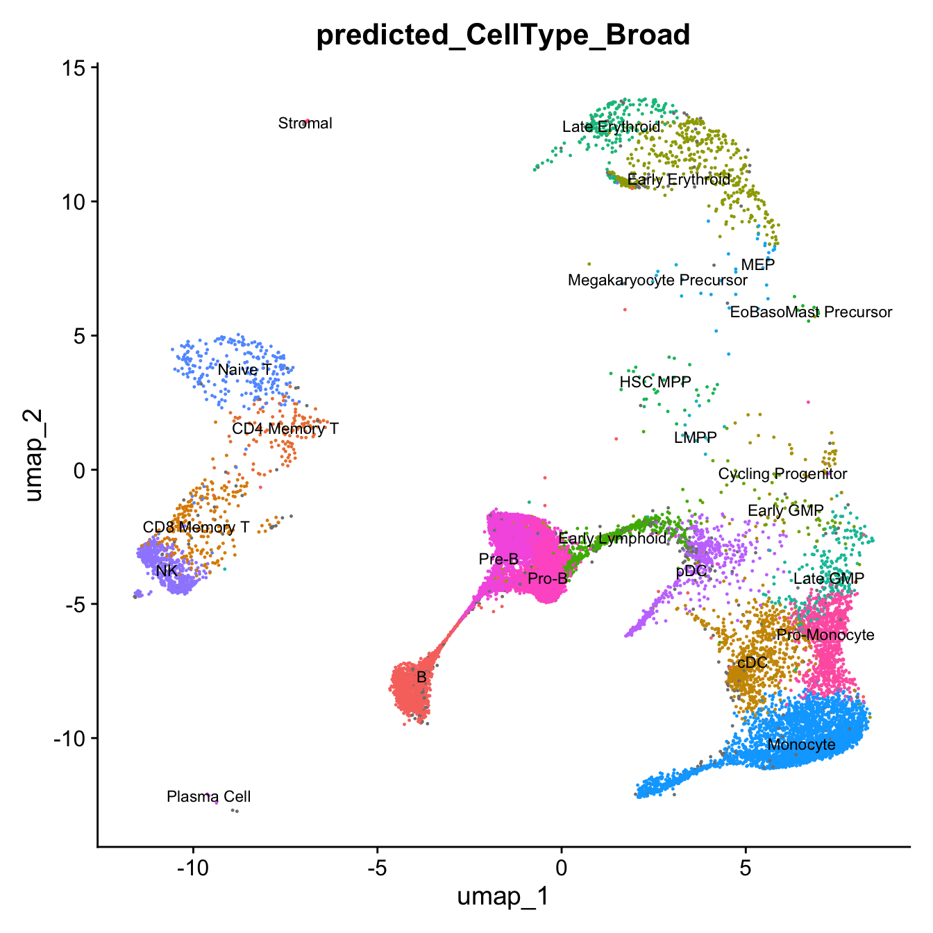
# Cache the BoneMarrowMap projection result (map_Query + predict_CellTypes).
# Loading this avoids re-running the Symphony projection on subsequent rebuilds.
out_proj <- here("data", "RDS", "ball_exp1_projected.seu.rds")
if(!file.exists(out_proj)) saveRDS(query, out_proj)
Exploratory UMAP overview
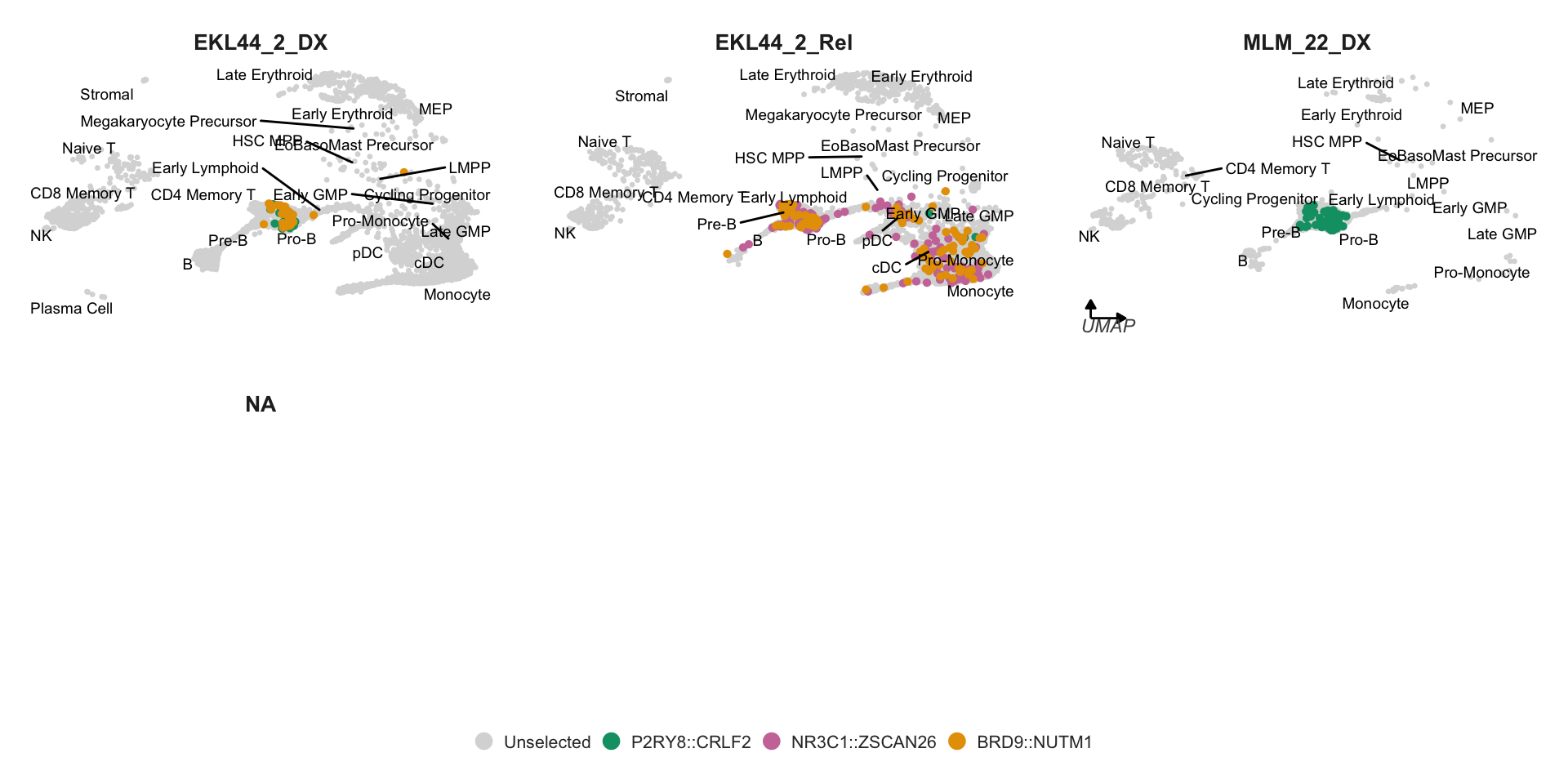
Per-sample projected UMAPs showing BoneMarrowMap broad cell type
labels and fusion-positive cells highlighted. These are diagnostic plots
confirming the projection and annotation quality; the
publication-quality Figure 3A–B panels are assembled in
B-ALL_exp1_clustering.Rmd.
# Figure 3A-B
query$predicted_CellType_Broad <- factor(
  ifelse(is.na(query$predicted_CellType_Broad), "Unassigned",
         as.character(query$predicted_CellType_Broad)),
  levels = c(
    "Pro-B", "Pre-B", "B", "Plasma Cell",
    "Early Lymphoid", "Naive T", "CD4 Memory T", "CD8 Memory T", "NK",
    "cDC", "pDC",
    "MEP", "Early Erythroid", "Late Erythroid",
    "Early GMP", "Late GMP", "Pro-Monocyte", "Monocyte",
    "HSC MPP", "LMPP", "Cycling Progenitor",
    "EoBasoMast Precursor", "Megakaryocyte Precursor",
    "Stromal", "Unassigned"
  )
)

cells.highlight <- split(which(query$patient_fusion != "not-detected"),
                                query$patient_fusion[query$patient_fusion != "not-detected"])


DimPlot(query, reduction = 'umap_projected',
        group.by = c('predicted_CellType_Broad'),
        split.by = "Sample",
        raster = FALSE,
        label = TRUE,
        label.size = 2.5,
        repel = T,
        cells.highlight = cells.highlight,
        cols.highlight = setNames(c("red","green","purple"),
                                  names(cells.highlight))) +
  theme(legend.position = "bottom") -> p1

p1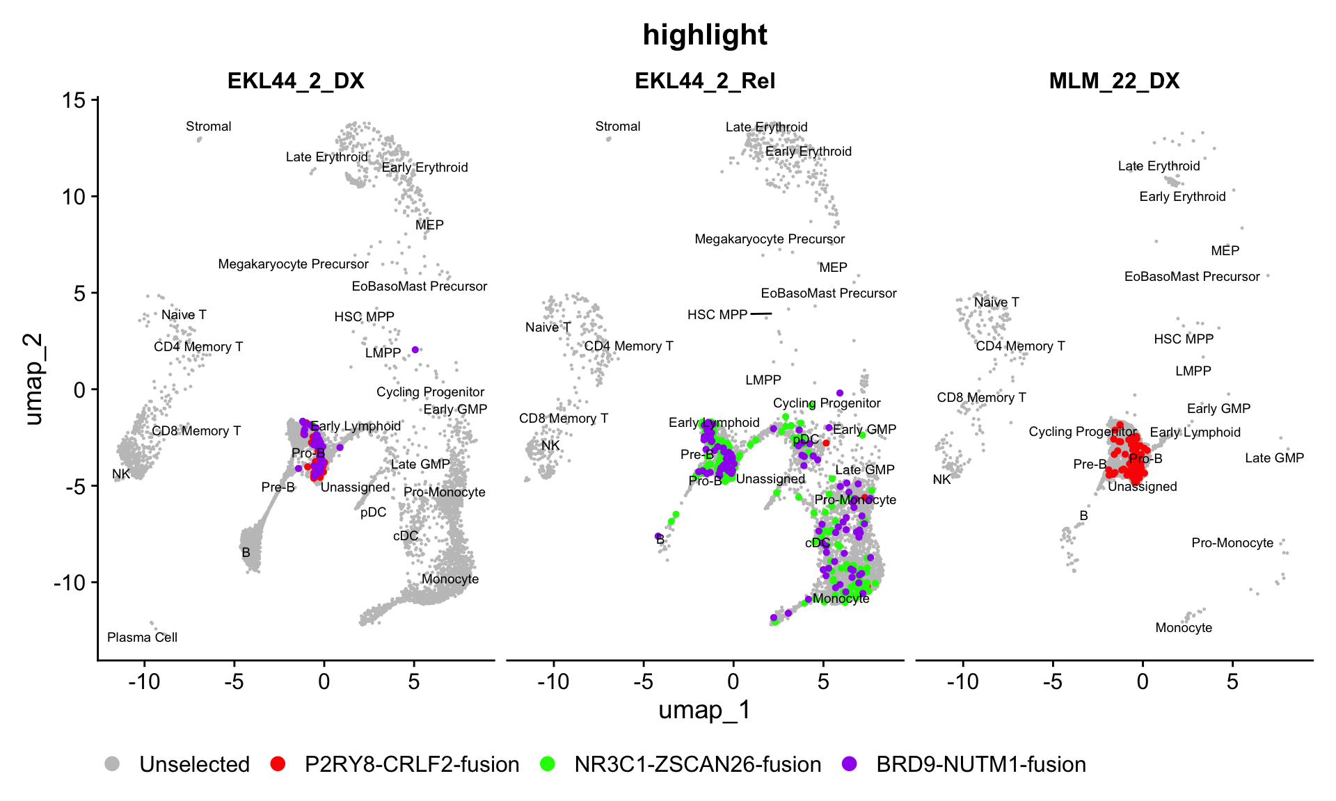
# ── Replace Unassigned with empty string to suppress label ────────────────────
query$predicted_CellType_Broad_plot <- dplyr::case_when(
  is.na(query$predicted_CellType_Broad)          ~ NA_character_,
  query$predicted_CellType_Broad == "Unassigned" ~ NA_character_,
  TRUE                                           ~ as.character(query$predicted_CellType_Broad)
)

# ── Clean fusion labels ───────────────────────────────────────────────────────
query$fusion_label <- dplyr::case_when(
  query$patient_fusion == "P2RY8-CRLF2-fusion"   ~ "P2RY8::CRLF2",
  query$patient_fusion == "NR3C1-ZSCAN26-fusion"  ~ "NR3C1::ZSCAN26",
  query$patient_fusion == "BRD9-NUTM1-fusion"     ~ "BRD9::NUTM1",
  TRUE                                            ~ "not-detected"
)

# ── Fusion colours ────────────────────────────────────────────────────────────
fusion_colours <- c(
  "P2RY8::CRLF2"   = "#E69F00",
  "NR3C1::ZSCAN26" = "#CC79A7",
  "BRD9::NUTM1"    = "#009E73"
)

# ── Cells to highlight ────────────────────────────────────────────────────────
cells_highlight <- split(
  which(query$fusion_label != "not-detected"),
  query$fusion_label[query$fusion_label != "not-detected"]
)

# ── UMAP coordinate range ─────────────────────────────────────────────────────
umap_coords  <- as.data.frame(query@reductions$umap_projected@cell.embeddings)
x_range_umap <- range(umap_coords[, 1])
y_range_umap <- range(umap_coords[, 2])
arrow_len_x  <- diff(x_range_umap) * 0.08
arrow_len_y  <- diff(y_range_umap) * 0.08

arrow_y <- y_range_umap[1] - 2.5
arrow_x <- x_range_umap[1]

# ── Plot ──────────────────────────────────────────────────────────────────────
DimPlot(
  query,
  reduction       = "umap_projected",
  group.by        = "predicted_CellType_Broad_plot",
  split.by        = "Sample",
  raster          = FALSE,
  label           = TRUE,
  label.size      = 2.5,
  repel           = TRUE,
  cells.highlight = cells_highlight,
  cols.highlight  = fusion_colours[names(cells_highlight)],
  cols            = "grey85",
  pt.size         = 0.4
) +

  # Horizontal arrow — MLM_22_DX panel only
  geom_segment(
    data = data.frame(
      predicted_CellType_Broad_plot = "",
      Sample = factor("MLM_22_DX", levels = levels(query$Sample))
    ),
    aes(x    = arrow_x,
        xend = arrow_x + arrow_len_x,
        y    = arrow_y,
        yend = arrow_y),
    arrow       = arrow(length = unit(0.15, "cm"), type = "closed"),
    linewidth   = 0.5, color = "black", inherit.aes = FALSE
  ) +

  # Vertical arrow — MLM_22_DX panel only
  geom_segment(
    data = data.frame(
      predicted_CellType_Broad_plot = "",
      Sample = factor("MLM_22_DX", levels = levels(query$Sample))
    ),
    aes(x    = arrow_x,
        xend = arrow_x,
        y    = arrow_y,
        yend = arrow_y + arrow_len_y),
    arrow       = arrow(length = unit(0.15, "cm"), type = "closed"),
    linewidth   = 0.5, color = "black", inherit.aes = FALSE
  ) +

  # UMAP label — MLM_22_DX panel only
  geom_text(
    data = data.frame(
      predicted_CellType_Broad_plot = "",
      Sample = factor("MLM_22_DX", levels = levels(query$Sample)),
      x      = arrow_x + arrow_len_x / 2,
      y      = arrow_y - diff(y_range_umap) * 0.03
    ),
    aes(x = x, y = y, label = "UMAP"),
    size        = 3,
    fontface    = "italic",
    color       = "grey30",
    hjust       = 0.5,
    inherit.aes = FALSE
  ) +

  labs(title = NULL) +
  theme_classic(base_size = 10) +
  theme(
    axis.title       = element_blank(),
    axis.text        = element_blank(),
    axis.ticks       = element_blank(),
    axis.line        = element_blank(),
    panel.grid       = element_blank(),
    panel.border     = element_blank(),
    panel.spacing    = unit(1.5, "lines"),
    strip.text       = element_text(size = 10, face = "bold", color = "grey15"),
    strip.background = element_blank(),
    legend.position  = "bottom",
    legend.title     = element_blank(),
    legend.text      = element_text(size = 8, color = "grey20"),
    legend.key.size  = unit(0.5, "lines")
  )
Bar chart showing the number of fusion-positive cells per sample for each of the three patient-specific fusions. Zero counts are included for sample/fusion combinations where no cells were detected.
# Figure 3D
fusion_sample_counts <- seu@meta.data %>%
  filter(patient_fusion != "not-detected") %>%
  mutate(
    fusion_label = dplyr::case_when(
      patient_fusion == "P2RY8-CRLF2-fusion"   ~ "P2RY8::CRLF2",
      patient_fusion == "NR3C1-ZSCAN26-fusion"  ~ "NR3C1::ZSCAN26",
      patient_fusion == "BRD9-NUTM1-fusion"     ~ "BRD9::NUTM1",
      TRUE                                      ~ patient_fusion
    )
  ) %>%
  group_by(Sample, fusion_label) %>%
  summarise(n_cells = n(), .groups = "drop") %>%
  # Complete to add zero rows for missing sample/fusion combinations
  complete(
    Sample       = c("MLM_22_DX", "EKL44_2_DX", "EKL44_2_Rel"),
    fusion_label = names(fusion_colours),
    fill         = list(n_cells = 0)
  ) %>%
  mutate(
    Sample       = factor(Sample, levels = c("MLM_22_DX", "EKL44_2_DX", "EKL44_2_Rel")),
    fusion_label = factor(fusion_label, levels = names(fusion_colours))
  )

ggplot(fusion_sample_counts,
       aes(x = Sample, y = n_cells, fill = fusion_label)) +
  geom_col(position = position_dodge(width = 0.75),
           width     = 0.65,
           color     = "white",
           linewidth = 0.3) +
  geom_text(
    aes(label = n_cells, y = n_cells),
    position = position_dodge(width = 0.75),
    vjust    = -0.4,
    size     = 2.8,
    color    = "grey30",
    fontface = "bold"
  ) +
  scale_fill_manual(values = fusion_colours, name = NULL) +
  scale_x_discrete(
    expand = expansion(add = 0.5),
    labels = c(
    "MLM_22_DX"   = "MLM_22_DX",
    "EKL44_2_DX"  = "EKL44_2_DX",
    "EKL44_2_Rel" = "EKL44_2_Rel"
  )) +
  # scale_y_continuous(
  #   expand = expansion(mult = c(0, 0.12)),
  #   limits = c(0, 200)
  # ) +
  labs(
    x     = NULL,
    y     = "No. fusion-positive cells",
    title = "Fusion-positive cell counts"
  ) +
  theme_classic(base_size = 10) +
  theme(
    plot.title         = element_text(size = 10, face = "bold", color = "grey15",
                                      margin = margin(b = 6)),
    axis.title.y       = element_text(size = 9, color = "grey20",
                                      margin = margin(r = 4)),
    axis.text.x        = element_text(size = 8, color = "grey20"),
    axis.text.y        = element_text(size = 8, color = "grey30"),
    axis.line          = element_line(color = "grey60", linewidth = 0.4),
    axis.ticks         = element_line(color = "grey60", linewidth = 0.3),
    panel.grid.major.y = element_line(color = "grey95", linewidth = 0.4),
    legend.position    = c(0.15, 0.85),
    legend.background  = element_rect(fill = "white", color = "grey85",
                                      linewidth = 0.3),
    legend.margin      = margin(3, 6, 3, 6),
    legend.text        = element_text(size = 9, color = "grey20"),
    legend.key.size    = unit(0.4, "lines"),
    plot.margin        = margin(6, 6, 6, 6)
  )
blast_types <- c("Pro-B", "Pre-B", "Early Lymphoid")
myeloid_types <- c(
  "B", "Plasma Cell",
  "Naive T", "CD4 Memory T", "CD8 Memory T", "NK",
  "cDC", "pDC",
  "MEP", "Early Erythroid", "Late Erythroid",
  "Early GMP", "Late GMP", "Pro-Monocyte", "Monocyte",
  "HSC MPP", "LMPP", "Cycling Progenitor",
  "EoBasoMast Precursor", "Megakaryocyte Precursor",
  "Stromal"
)

# Updated groupings - sample-specific facets
query$marker_group <- dplyr::case_when(
  query$patient_fusion != "not-detected" &
    query$predicted_CellType_Broad %in% blast_types              ~ "Fn+\nBlast",
  query$Sample == "EKL44_2_Rel" &
    query$patient_fusion != "not-detected" &
    query$predicted_CellType_Broad %in% myeloid_types            ~ "Fn+\nMyeloid",
  query$Sample == "EKL44_2_Rel" &
    query$patient_fusion != "not-detected" &
    query$predicted_CellType_Broad == "Unassigned"               ~ "Fn+\nUnassigned",
  query$patient_fusion == "not-detected" &
    query$predicted_CellType_Broad %in% blast_types              ~ "Fn-\nBlast",
  query$patient_fusion == "not-detected" &
    !query$predicted_CellType_Broad %in% blast_types             ~ "Fn-\n(non-blast)",
  TRUE ~ NA_character_
)

group_levels <- c("Fn+\nBlast", "Fn+\nMyeloid", "Fn+\nUnassigned",
                  "Fn-\nBlast", "Fn-\n(non-blast)")

# Facet order: MLM first, then EKL44 DX, then EKL44 Rel
query$marker_facet <- factor(
  query$Sample,
  levels = c("MLM_22_DX", "EKL44_2_DX", "EKL44_2_Rel")
)

markers <- c("CD19", "DNTT", "MME", "CD34", "CD14", "HBB")

marker_counts <- GetAssayData(query, layer = "counts")[markers, ]
marker_norm   <- GetAssayData(query, layer = "data")[markers, ]

dot_df_c1 <- query@meta.data %>%
  tibble::rownames_to_column("cell") %>%
  filter(!is.na(marker_group)) %>%
  select(cell, marker_group, marker_facet) %>%
  { df <- .
    lapply(markers, function(gn) {
      counts_vec <- as.numeric(marker_counts[gn, df$cell])
      norm_vec   <- as.numeric(marker_norm[gn, df$cell])
      df %>%
        mutate(
          expressed = counts_vec > 0,
          norm_expr = norm_vec
        ) %>%
        group_by(marker_group, marker_facet) %>%
        summarise(
          pct_expressing = mean(expressed) * 100,
          mean_expr      = ifelse(any(expressed),
                                  mean(norm_expr[expressed]), NA_real_),
          n = n(),
          .groups = "drop"
        ) %>%
        mutate(marker = gn)
    }) %>%
      bind_rows()
  } %>%
  mutate(
    marker       = factor(marker, levels = rev(markers)),
    marker_group = factor(marker_group, levels = group_levels),
    marker_facet = factor(marker_facet,
                          levels = c("MLM_22_DX", "EKL44_2_DX", "EKL44_2_Rel"))
  ) %>%
  # Drop combinations that don't exist
  # (e.g. Myeloid/Unassigned in MLM_22 and EKL44_DX)
  filter(!is.na(pct_expressing) | !is.na(mean_expr))

# n labels
group_n <- query@meta.data %>%
  filter(!is.na(marker_group), !is.na(marker_facet)) %>%
  group_by(marker_group, marker_facet) %>%
  summarise(n = n(), .groups = "drop") %>%
  mutate(
    marker_group = factor(marker_group, levels = group_levels),
    marker_facet = factor(marker_facet,
                          levels = c("MLM_22_DX", "EKL44_2_DX", "EKL44_2_Rel")),
    label = paste0("n=", scales::comma(n))
  )

# Dashed line only in EKL44_Rel facet after Unassigned
vline_df <- data.frame(
  marker_facet = factor("EKL44_2_Rel",
                        levels = c("MLM_22_DX", "EKL44_2_DX", "EKL44_2_Rel")),
  xintercept   = 3.5
)

ggplot(dot_df_c1 %>% filter(!is.na(marker_group)),
       aes(x = marker_group, y = marker,
           size = pct_expressing, colour = mean_expr)) +
  geom_point(alpha = 0.9) +
   # n labels at top of each column
  geom_text(
    data        = group_n,
    aes(x = marker_group, y = Inf, label = label),
    inherit.aes = FALSE,
    vjust       = 0.75,
    size        = 2.3,
    colour      = "grey40",
    fontface    = "italic"
  ) +
  geom_vline(
    data      = vline_df,
    aes(xintercept = xintercept),
    linetype  = "dashed",
    colour    = "grey60",
    linewidth = 0.4
  ) +
  facet_grid(
    cols   = vars(marker_facet),
    scales = "free_x",
    space  = "free_x"
  ) +
  scale_colour_gradient(
    low      = "#E8D5F0",
    high     = "#4A0080",
    name     = "Mean\nexpr.",
    na.value = "grey80",
    guide    = guide_colourbar(direction      = "horizontal",
                               title.position = "left",
                               barwidth       = 4,
                               barheight      = 0.5)
  ) +
  scale_size_continuous(
    name   = "% expr.",
    range  = c(0.5, 8),
    breaks = c(1, 25, 50, 75),
    limits = c(0, 100),
    guide  = guide_legend(direction      = "horizontal",
                          title.position = "left",
                          nrow           = 1)
  ) +
  coord_cartesian(clip = "off") +
  labs(x = NULL, y = NULL,
       title = "Marker expression by fusion-positive cell type") +
  theme_classic(base_size = 11) +
  theme(
    plot.title       = element_text(size = 11, face = "bold", colour = "grey15",
                                    hjust = 0.5, margin = margin(b = 6)),
    axis.text.x      = element_text(size = 7, colour = "grey15", hjust = 0.5),
    axis.text.y      = element_text(size = 9, colour = "grey15"),
    panel.grid.major = element_line(colour = "grey92", linewidth = 0.3),
    strip.background = element_blank(),
    strip.text       = element_text(size = 10, face = "bold", colour = "grey15"),
    legend.position  = "bottom",
    legend.box       = "horizontal",
    legend.direction = "horizontal",
    plot.margin      = margin(20, 6, 6, 6),
    panel.spacing    = unit(1, "lines")
  )
Pseudotime and projection density
Pseudotime scores are transferred from the BoneMarrowMap reference by KNN assignment in projected UMAP space. Projection density plots show how query cells distribute across the haematopoietic hierarchy relative to the reference, computed per sample. Query cells will be assigned a pseudotime score based on the 30 K-Nearest Neighbours from the reference map. Since our Pseudotime KNN assignments are performed in UMAP space (more accurate than KNN on harmony components), this step is very fast (< 10s)
# Predict Pseudotime values by KNN
query <- predict_Pseudotime(
  query_obj = query,
  ref_obj = ref,
  initial_label = 'initial_Pseudotime',  # pseudotime assignments before filtering on mapping QC
  final_label = 'predicted_Pseudotime'   # pseudotime assignments with map QC failing cells assigned as NA
)

# Visualize Hematopoietic Pseudotime in query data
plots <- FeaturePlot(query,
                     features = c('predicted_Pseudotime'),
                     split.by = 'Sample',
                     combine = FALSE)

patchwork::wrap_plots(lapply(plots, function(p) {
  p + scale_color_gradientn(colors = rev(RColorBrewer::brewer.pal(11, 'RdBu')))
}), guides = "collect", ncol = 2)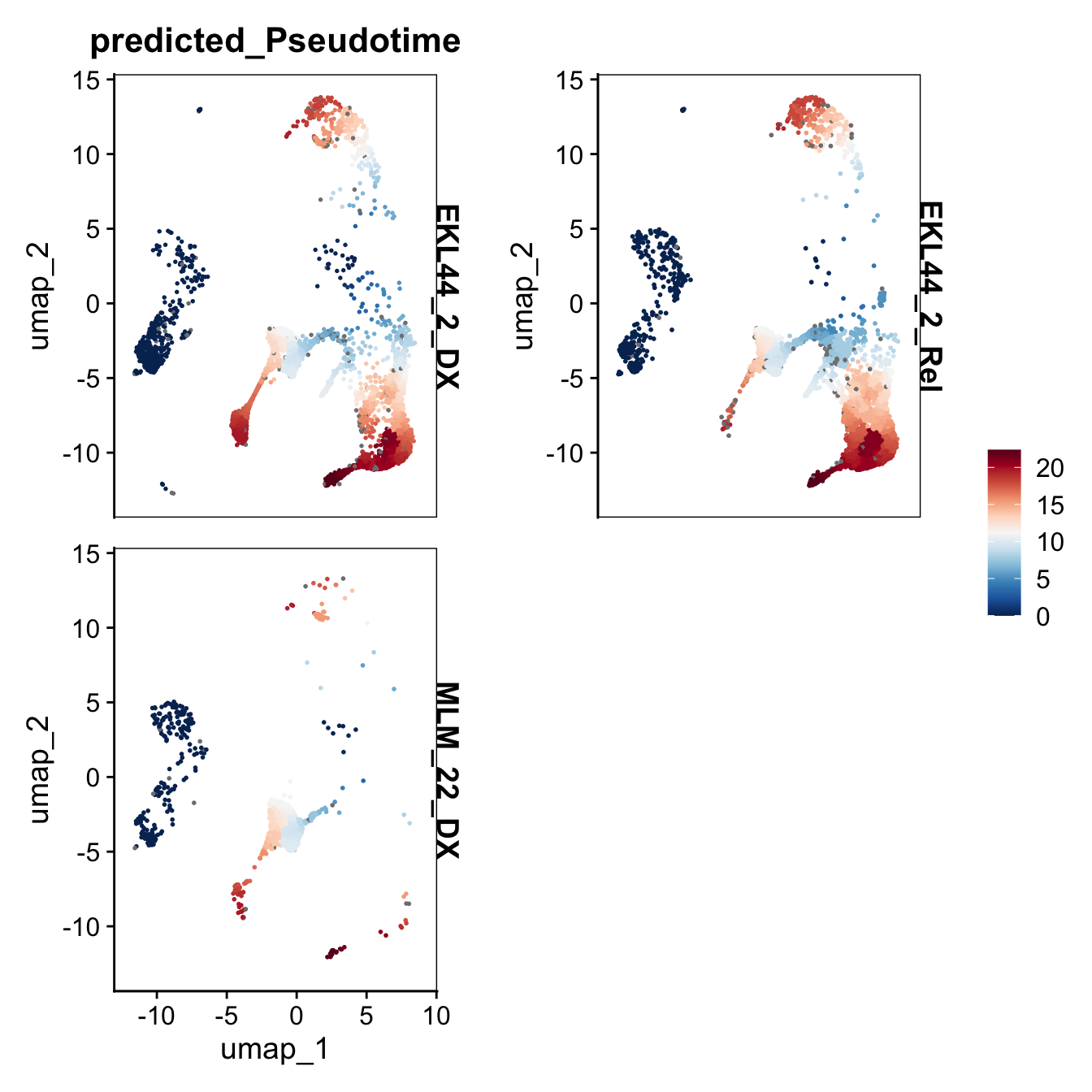
Projection density
# Set batch/condition to be visualized individually
batch_key <- 'Sample'

# returns a list of plots for each donor from a pre-specified batch variable
projection_plots <- plot_Projection_byDonor(
  query_obj = query,
  batch_key = batch_key,
  ref_obj = ref,
  Hierarchy_only = FALSE, # Whether to exclude T/NK/Plasma/Stromal cells
  downsample_reference = TRUE,
  downsample_frac = 0.25,   # down-sample reference cells to 25%; reduces figure file size
  query_point_size = 0.2,   # adjust size of query cells based on # of cells
  saveplot = TRUE,
  save_folder = 'projectionFigures/'
)

# show plots together with patchwork. Can also just call "projection_plots" object to display one-by-one
patchwork::wrap_plots(projection_plots, ncol = 3)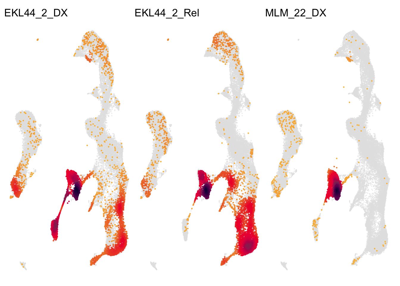
Cell type composition per sample
Cell type abundance per sample, restricted to cells with KNN classification probability > 0.5 (i.e. > 50% of nearest reference neighbours agree on the assigned label).
query_composition <- get_Composition(
  query_obj = query,
  donor_key = 'Sample',
  celltype_label = 'predicted_CellType',
  mapQC_col = 'mapping_error_QC',
  knn_prob_cutoff = 0.5,
  return_type = 'long')

query_composition
# A tibble: 140 × 4
Sample predicted_CellType count proportion
<fct> <chr> <int> <dbl>
1 EKL44_2_DX Pro-B VDJ 2177 0.240
2 EKL44_2_DX Small Pre-B 994 0.110
3 EKL44_2_DX Mature B 882 0.0974
4 EKL44_2_DX CD14 Mono 866 0.0956
5 EKL44_2_DX Large Pre-B 697 0.0770
6 EKL44_2_DX Immature B 591 0.0653
7 EKL44_2_DX Pro-B Cycling 493 0.0544
8 EKL44_2_DX Early ProMono 355 0.0392
9 EKL44_2_DX CD16 Mono 221 0.0244
10 EKL44_2_DX NK 212 0.0234
# ℹ 130 more rowsquery_composition %>%
dplyr::filter(proportion > 0.01) %>%
mutate(predicted_CellType = fct_drop(predicted_CellType)) %>%
ggplot(aes(x = Sample, y = proportion, fill= predicted_CellType)) +
geom_bar(stat = "identity", outline = 1) +
paletteer::scale_fill_paletteer_d(palette = "ggthemes::Tableau_20") +
guides(fill = guide_legend(ncol = 3)) +
theme(legend.position = "bottom")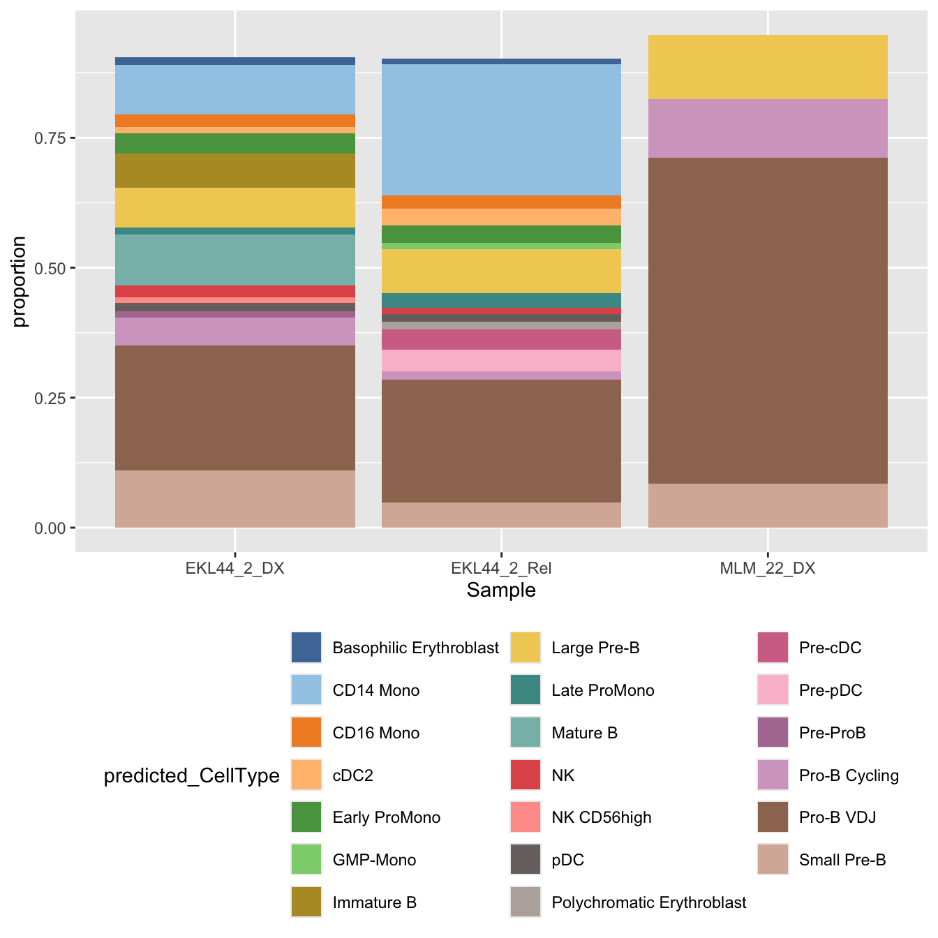
Or as a wide table with counts of # of cells
query_composition_wide_counts <- get_Composition(
  query_obj = query,
  donor_key = 'Sample',
  celltype_label = 'predicted_CellType',
  mapQC_col = 'mapping_error_QC',
  knn_prob_cutoff = 0.5,
  return_type = 'count')

query_composition_wide_counts
# A tibble: 3 × 55
Sample `Pro-B VDJ` `Small Pre-B` `Mature B` `CD14 Mono` `Large Pre-B`
<fct> <int> <int> <int> <int> <int>
1 EKL44_2_DX 2177 994 882 866 697
2 EKL44_2_Rel 1525 313 13 1623 546
3 MLM_22_DX 4800 647 32 6 945
# ℹ 49 more variables: `Immature B` <int>, `Pro-B Cycling` <int>,
# `Early ProMono` <int>, `CD16 Mono` <int>, NK <int>,
# `Basophilic Erythroblast` <int>, pDC <int>, `Late ProMono` <int>,
# `Pre-ProB` <int>, cDC2 <int>, `NK CD56high` <int>, `GMP-Mono` <int>,
# `Pre-cDC` <int>, `Pro-Erythroblast` <int>, CLP <int>,
# `Polychromatic Erythroblast` <int>, `CFU-E` <int>,
# `CD8 Effector Memory 1` <int>, `CD8 Effector Memory 2` <int>, …Or as a wide table with proportion of each cell type within each donor
query_composition_wide_props <- get_Composition(
  query_obj = query,
  donor_key = 'Sample',
  celltype_label = 'predicted_CellType',
  mapQC_col = 'mapping_error_QC',
  knn_prob_cutoff = 0.5,
  return_type = 'proportion')

query_composition_wide_props
# A tibble: 3 × 55
Sample `Pro-B VDJ` `Small Pre-B` `Mature B` `CD14 Mono` `Large Pre-B`
<fct> <dbl> <dbl> <dbl> <dbl> <dbl>
1 EKL44_2_DX 0.240 0.110 0.0974 0.0956 0.0770
2 EKL44_2_Rel 0.237 0.0486 0.00202 0.252 0.0847
3 MLM_22_DX 0.627 0.0845 0.00418 0.000784 0.123
# ℹ 49 more variables: `Immature B` <dbl>, `Pro-B Cycling` <dbl>,
# `Early ProMono` <dbl>, `CD16 Mono` <dbl>, NK <dbl>,
# `Basophilic Erythroblast` <dbl>, pDC <dbl>, `Late ProMono` <dbl>,
# `Pre-ProB` <dbl>, cDC2 <dbl>, `NK CD56high` <dbl>, `GMP-Mono` <dbl>,
# `Pre-cDC` <dbl>, `Pro-Erythroblast` <dbl>, CLP <dbl>,
# `Polychromatic Erythroblast` <dbl>, `CFU-E` <dbl>,
# `CD8 Effector Memory 1` <dbl>, `CD8 Effector Memory 2` <dbl>, …Heatmap of cell type composition by sample.
# Simple heatmap to visualize composition of projected samples
p <- query_composition_wide_props %>%
  # show celltypes present in >1% of total cells
  select(Sample,
         colnames(query_composition_wide_props)[-1][colSums(query_composition_wide_props[-1]) > 0.01]) %>%
  # convert to matrix and display heatmap
  column_to_rownames('Sample') %>% data.matrix() %>% ComplexHeatmap::Heatmap()
p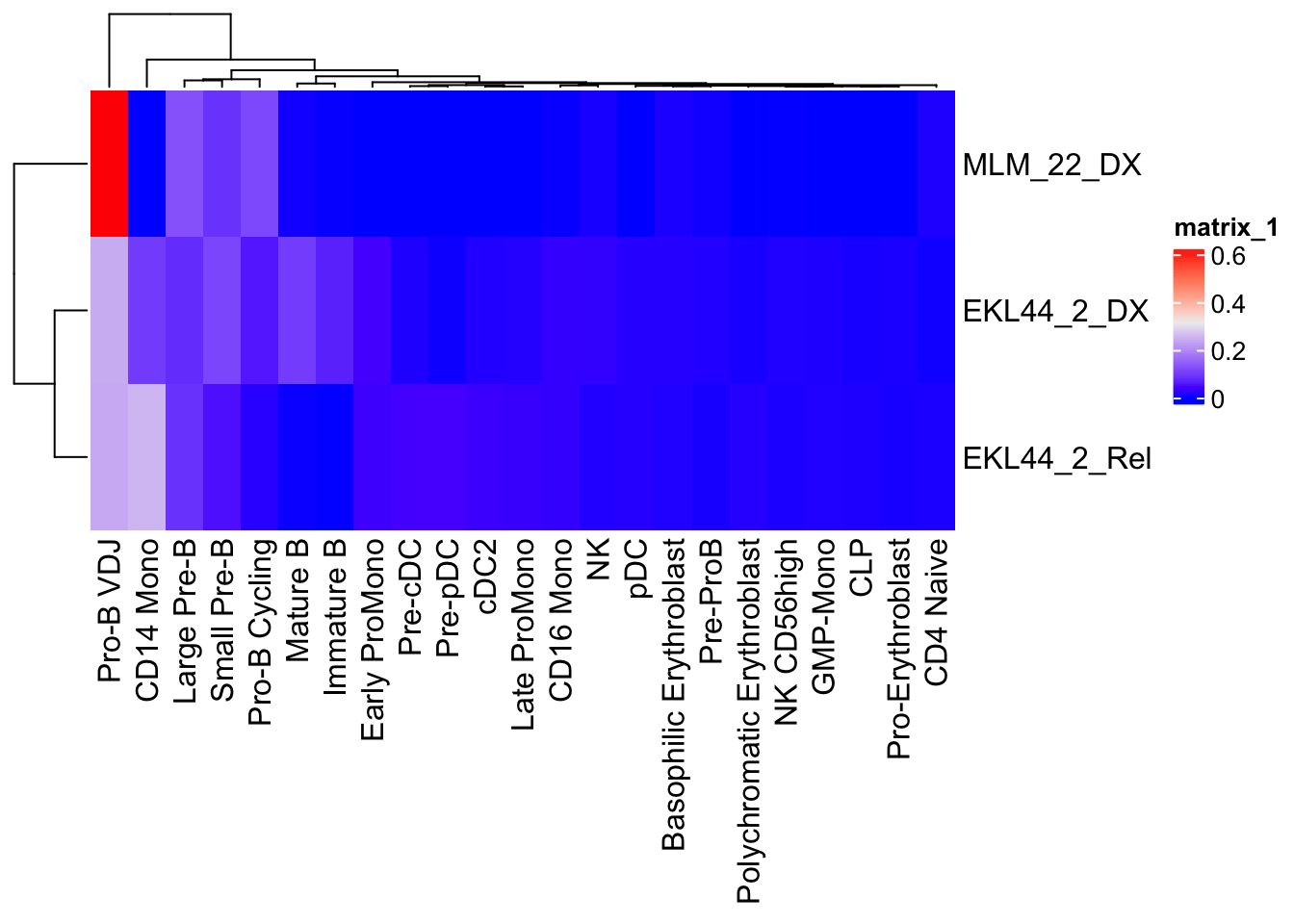
Save data
out <- here("data", "RDS", "ball_exp1_annotated.seu.rds")
if(!file.exists(out)) saveRDS(query, out)
fs::file_chmod(out, "664")
try(fs::file_chown(out, group_id = "oshlack_lab"),
    silent = TRUE)
Session info
sessioninfo::session_info()─ Session info ───────────────────────────────────────────────────────────────
setting value
version R version 4.4.1 (2024-06-14)
os macOS 15.5
system aarch64, darwin20
ui X11
language (EN)
collate en_US.UTF-8
ctype en_US.UTF-8
tz Australia/Melbourne
date 2026-07-15
pandoc 3.8.3 @ /Applications/RStudio.app/Contents/Resources/app/quarto/bin/tools/aarch64/ (via rmarkdown)
quarto 1.9.38 @ /Applications/RStudio.app/Contents/Resources/app/quarto/bin/quarto
─ Packages ───────────────────────────────────────────────────────────────────
! package * version date (UTC) lib source
P abind 1.4-8 2024-09-12 [?] CRAN (R 4.4.1)
P annotate 1.84.0 2024-11-08 [?] Bioconduc~
P AnnotationDbi 1.68.0 2024-11-08 [?] Bioconduc~
AUCell 1.28.0 2024-11-08 [1] Bioconductor 3.20 (R 4.4.1)
P backports 1.5.0 2024-05-23 [?] CRAN (R 4.4.1)
P beeswarm 0.4.0 2021-06-01 [?] CRAN (R 4.4.1)
P Biobase * 2.66.0 2024-11-08 [?] Bioconduc~
P BiocGenerics * 0.52.0 2024-11-08 [?] Bioconduc~
P BiocManager 1.30.27 2025-11-14 [?] CRAN (R 4.4.3)
P BiocNeighbors 2.0.1 2024-11-28 [?] Bioconduc~
P Biostrings 2.74.1 2024-12-16 [?] Bioconduc~
P bit 4.6.0 2025-03-06 [?] CRAN (R 4.4.1)
P bit64 4.6.0-1 2025-01-16 [?] CRAN (R 4.4.1)
P blob 1.2.4 2023-03-17 [?] CRAN (R 4.4.0)
BoneMarrowMap * 0.1.0 2025-06-04 [1] Github (andygxzeng/BoneMarrowMap@81f2756)
P broom 1.0.8 2025-03-28 [?] CRAN (R 4.4.1)
P bslib 0.9.0 2025-01-30 [?] CRAN (R 4.4.1)
P cachem 1.1.0 2024-05-16 [?] CRAN (R 4.4.1)
P Cairo 1.6-2 2023-11-28 [?] CRAN (R 4.4.1)
P callr 3.7.6 2024-03-25 [?] CRAN (R 4.4.0)
P car 3.1-3 2024-09-27 [?] CRAN (R 4.4.1)
P carData 3.0-5 2022-01-06 [?] CRAN (R 4.4.1)
P circlize 0.4.16 2024-02-20 [?] CRAN (R 4.4.0)
P cli 3.6.5 2025-04-23 [?] CRAN (R 4.4.1)
P clue 0.3-66 2024-11-13 [?] CRAN (R 4.4.1)
P cluster 2.1.6 2023-12-01 [?] CRAN (R 4.4.1)
P codetools 0.2-20 2024-03-31 [?] CRAN (R 4.4.1)
P colorspace 2.1-1 2024-07-26 [?] CRAN (R 4.4.1)
P ComplexHeatmap 2.22.0 2024-11-08 [?] Bioconduc~
P cowplot 1.1.3 2024-01-22 [?] CRAN (R 4.4.0)
P crayon 1.5.3 2024-06-20 [?] CRAN (R 4.4.1)
P data.table 1.18.2.1 2026-01-27 [?] CRAN (R 4.4.3)
P DBI 1.2.3 2024-06-02 [?] CRAN (R 4.4.1)
P DelayedArray 0.32.0 2024-11-08 [?] Bioconduc~
P DelayedMatrixStats 1.28.1 2025-01-09 [?] Bioconduc~
P deldir 2.0-4 2024-02-28 [?] CRAN (R 4.4.1)
P digest 0.6.37 2024-08-19 [?] CRAN (R 4.4.1)
P doParallel 1.0.17 2022-02-07 [?] CRAN (R 4.4.0)
P dotCall64 1.2 2024-10-04 [?] CRAN (R 4.4.1)
P dplyr * 1.1.4 2023-11-17 [?] CRAN (R 4.4.0)
P evaluate 1.0.3 2025-01-10 [?] CRAN (R 4.4.1)
P farver 2.1.2 2024-05-13 [?] CRAN (R 4.4.1)
P fastDummies 1.7.5 2025-01-20 [?] CRAN (R 4.4.1)
P fastmap 1.2.0 2024-05-15 [?] CRAN (R 4.4.1)
P fitdistrplus 1.2-2 2025-01-07 [?] CRAN (R 4.4.1)
P forcats * 1.0.0 2023-01-29 [?] CRAN (R 4.4.0)
P foreach 1.5.2 2022-02-02 [?] CRAN (R 4.4.0)
P Formula 1.2-5 2023-02-24 [?] CRAN (R 4.4.1)
P fs 1.6.6 2025-04-12 [?] CRAN (R 4.4.1)
P future 1.49.0 2025-05-09 [?] CRAN (R 4.4.1)
P future.apply 1.11.3 2024-10-27 [?] CRAN (R 4.4.1)
P generics 0.1.4 2025-05-09 [?] CRAN (R 4.4.1)
P GenomeInfoDb * 1.42.3 2025-01-27 [?] Bioconduc~
P GenomeInfoDbData 1.2.13 2025-05-28 [?] Bioconductor
P GenomicRanges * 1.58.0 2024-11-08 [?] Bioconduc~
P GetoptLong 1.0.5 2020-12-15 [?] CRAN (R 4.4.1)
P getPass 0.2-4 2023-12-10 [?] CRAN (R 4.4.1)
P ggbeeswarm 0.7.2 2023-04-29 [?] CRAN (R 4.4.0)
P ggplot2 * 4.0.2 2026-02-03 [?] CRAN (R 4.4.3)
ggpointdensity 0.2.0 2025-05-16 [1] CRAN (R 4.4.1)
P ggpubr 0.6.0 2023-02-10 [?] CRAN (R 4.4.0)
P ggrastr 1.0.2 2023-06-01 [?] CRAN (R 4.4.0)
P ggrepel 0.9.6 2024-09-07 [?] CRAN (R 4.4.1)
P ggridges 0.5.6 2024-01-23 [?] CRAN (R 4.4.0)
P ggsignif 0.6.4 2022-10-13 [?] CRAN (R 4.4.0)
P git2r 0.36.2 2025-03-29 [?] CRAN (R 4.4.1)
P GlobalOptions 0.1.2 2020-06-10 [?] CRAN (R 4.4.1)
P globals 0.18.0 2025-05-08 [?] CRAN (R 4.4.1)
P glue * 1.8.0 2024-09-30 [?] CRAN (R 4.4.1)
P goftest 1.2-3 2021-10-07 [?] CRAN (R 4.4.1)
graph 1.84.1 2025-01-02 [1] Bioconductor 3.20 (R 4.4.2)
P gridExtra 2.3 2017-09-09 [?] CRAN (R 4.4.1)
GSEABase 1.68.0 2024-11-08 [1] Bioconductor 3.20 (R 4.4.1)
P gtable 0.3.6 2024-10-25 [?] CRAN (R 4.4.1)
P harmony 1.2.3 2024-11-27 [?] CRAN (R 4.4.1)
P here * 1.0.1 2020-12-13 [?] CRAN (R 4.4.1)
P hms 1.1.3 2023-03-21 [?] CRAN (R 4.4.0)
P htmltools 0.5.8.1 2024-04-04 [?] CRAN (R 4.4.1)
P htmlwidgets 1.6.4 2023-12-06 [?] CRAN (R 4.4.0)
P httpuv 1.6.16 2025-04-16 [?] CRAN (R 4.4.1)
P httr 1.4.7 2023-08-15 [?] CRAN (R 4.4.0)
P ica 1.0-3 2022-07-08 [?] CRAN (R 4.4.1)
P igraph 2.1.4 2025-01-23 [?] CRAN (R 4.4.1)
P IRanges * 2.40.1 2024-12-05 [?] Bioconduc~
P irlba 2.3.5.1 2022-10-03 [?] CRAN (R 4.4.0)
P iterators 1.0.14 2022-02-05 [?] CRAN (R 4.4.1)
jcolors 0.0.5 2025-06-04 [1] Github (jaredhuling/jcolors@7c29a50)
P jquerylib 0.1.4 2021-04-26 [?] CRAN (R 4.4.0)
P jsonlite 2.0.0 2025-03-27 [?] CRAN (R 4.4.1)
P KEGGREST 1.46.0 2024-11-08 [?] Bioconduc~
P KernSmooth 2.23-24 2024-05-17 [?] CRAN (R 4.4.1)
P knitr 1.50 2025-03-16 [?] CRAN (R 4.4.1)
P labeling 0.4.3 2023-08-29 [?] CRAN (R 4.4.1)
P later 1.4.2 2025-04-08 [?] CRAN (R 4.4.1)
P lattice 0.22-6 2024-03-20 [?] CRAN (R 4.4.1)
P lazyeval 0.2.2 2019-03-15 [?] CRAN (R 4.4.1)
P lifecycle 1.0.4 2023-11-07 [?] CRAN (R 4.4.1)
P listenv 0.9.1 2024-01-29 [?] CRAN (R 4.4.1)
P lmtest 0.9-40 2022-03-21 [?] CRAN (R 4.4.1)
P lubridate * 1.9.4 2024-12-08 [?] CRAN (R 4.4.1)
P magrittr 2.0.3 2022-03-30 [?] CRAN (R 4.4.1)
P MASS 7.3-60.2 2024-04-26 [?] CRAN (R 4.4.1)
P Matrix 1.7-0 2024-04-26 [?] CRAN (R 4.4.1)
P MatrixGenerics * 1.18.1 2025-01-09 [?] Bioconduc~
P matrixStats * 1.5.0 2025-01-07 [?] CRAN (R 4.4.1)
P memoise 2.0.1 2021-11-26 [?] CRAN (R 4.4.0)
P mime 0.13 2025-03-17 [?] CRAN (R 4.4.1)
P miniUI 0.1.2 2025-04-17 [?] CRAN (R 4.4.1)
P nlme 3.1-164 2023-11-27 [?] CRAN (R 4.4.1)
P paletteer 1.6.0 2024-01-21 [?] CRAN (R 4.4.0)
P parallelly 1.45.0 2025-06-02 [?] CRAN (R 4.4.1)
P patchwork * 1.3.0 2024-09-16 [?] CRAN (R 4.4.1)
P pbapply 1.7-4 2025-07-20 [?] CRAN (R 4.4.1)
P pillar 1.10.2 2025-04-05 [?] CRAN (R 4.4.1)
P pkgconfig 2.0.3 2019-09-22 [?] CRAN (R 4.4.1)
P plotly 4.10.4 2024-01-13 [?] CRAN (R 4.4.0)
P plyr 1.8.9 2023-10-02 [?] CRAN (R 4.4.1)
P png 0.1-8 2022-11-29 [?] CRAN (R 4.4.1)
P polyclip 1.10-7 2024-07-23 [?] CRAN (R 4.4.1)
P prismatic 1.1.2 2024-04-10 [?] CRAN (R 4.4.1)
P processx 3.8.6 2025-02-21 [?] CRAN (R 4.4.1)
P progressr 0.15.1 2024-11-22 [?] CRAN (R 4.4.1)
P promises 1.3.3 2025-05-29 [?] CRAN (R 4.4.1)
P ps 1.9.1 2025-04-12 [?] CRAN (R 4.4.1)
P purrr * 1.0.4 2025-02-05 [?] CRAN (R 4.4.1)
P R.methodsS3 1.8.2 2022-06-13 [?] CRAN (R 4.4.1)
P R.oo 1.27.1 2025-05-02 [?] CRAN (R 4.4.1)
P R.utils 2.13.0 2025-02-24 [?] CRAN (R 4.4.1)
P R6 2.6.1 2025-02-15 [?] CRAN (R 4.4.1)
P ragg 1.4.0 2025-04-10 [?] CRAN (R 4.4.1)
P RANN 2.6.2 2024-08-25 [?] CRAN (R 4.4.1)
P RColorBrewer 1.1-3 2022-04-03 [?] CRAN (R 4.4.1)
P Rcpp 1.1.1-1.1 2026-04-24 [?] CRAN (R 4.4.1)
P RcppAnnoy 0.0.22 2024-01-23 [?] CRAN (R 4.4.1)
P RcppHNSW 0.6.0 2024-02-04 [?] CRAN (R 4.4.1)
P readr * 2.1.5 2024-01-10 [?] CRAN (R 4.4.0)
P rematch2 2.1.2 2020-05-01 [?] CRAN (R 4.4.0)
renv 1.1.4 2025-03-20 [1] CRAN (R 4.4.1)
P reshape2 1.4.4 2020-04-09 [?] CRAN (R 4.4.0)
P reticulate 1.42.0 2025-03-25 [?] CRAN (R 4.4.1)
P rjson 0.2.23 2024-09-16 [?] CRAN (R 4.4.1)
P rlang 1.1.6 2025-04-11 [?] CRAN (R 4.4.1)
P rmarkdown 2.29 2024-11-04 [?] CRAN (R 4.4.1)
P ROCR 1.0-11 2020-05-02 [?] CRAN (R 4.4.0)
P rprojroot 2.0.4 2023-11-05 [?] CRAN (R 4.4.1)
P RSpectra 0.16-2 2024-07-18 [?] CRAN (R 4.4.0)
P RSQLite 2.4.0 2025-05-31 [?] CRAN (R 4.4.1)
P rstatix 0.7.2 2023-02-01 [?] CRAN (R 4.4.0)
P rstudioapi 0.17.1 2024-10-22 [?] CRAN (R 4.4.1)
P Rtsne 0.17 2023-12-07 [?] CRAN (R 4.4.1)
P S4Arrays 1.6.0 2024-11-08 [?] Bioconduc~
P S4Vectors * 0.44.0 2024-11-08 [?] Bioconduc~
P S7 0.2.0 2024-11-07 [?] CRAN (R 4.4.1)
P sass 0.4.10 2025-04-11 [?] CRAN (R 4.4.1)
P scales * 1.4.0 2025-04-24 [?] CRAN (R 4.4.1)
P scattermore 1.2 2023-06-12 [?] CRAN (R 4.4.0)
P sctransform 0.4.2 2025-04-30 [?] CRAN (R 4.4.1)
P sessioninfo 1.2.3 2025-02-05 [?] CRAN (R 4.4.1)
P Seurat * 5.3.0 2025-04-23 [?] CRAN (R 4.4.1)
P SeuratObject * 5.1.0 2025-04-22 [?] CRAN (R 4.4.1)
P shape 1.4.6.1 2024-02-23 [?] CRAN (R 4.4.1)
P shiny 1.10.0 2024-12-14 [?] CRAN (R 4.4.1)
P SingleCellExperiment * 1.28.1 2024-11-23 [?] Bioconduc~
P sp * 2.2-0 2025-02-01 [?] CRAN (R 4.4.1)
P spam 2.11-1 2025-01-20 [?] CRAN (R 4.4.1)
P SparseArray 1.6.2 2025-02-20 [?] Bioconduc~
P sparseMatrixStats 1.18.0 2024-11-08 [?] Bioconduc~
P spatstat.data 3.1-6 2025-03-17 [?] CRAN (R 4.4.1)
P spatstat.explore 3.4-3 2025-05-21 [?] CRAN (R 4.4.1)
P spatstat.geom 3.4-1 2025-05-20 [?] CRAN (R 4.4.1)
P spatstat.random 3.4-1 2025-05-20 [?] CRAN (R 4.4.1)
P spatstat.sparse 3.1-0 2024-06-21 [?] CRAN (R 4.4.0)
P spatstat.univar 3.1-3 2025-05-08 [?] CRAN (R 4.4.1)
P spatstat.utils 3.1-4 2025-05-15 [?] CRAN (R 4.4.1)
P stringi 1.8.7 2025-03-27 [?] CRAN (R 4.4.1)
P stringr * 1.6.0 2025-11-04 [?] CRAN (R 4.4.1)
P SummarizedExperiment * 1.36.0 2024-11-08 [?] Bioconduc~
P survival 3.6-4 2024-04-24 [?] CRAN (R 4.4.1)
P symphony * 0.1.1 2023-01-16 [?] CRAN (R 4.4.0)
P systemfonts 1.2.3 2025-04-30 [?] CRAN (R 4.4.1)
P tensor 1.5 2012-05-05 [?] CRAN (R 4.4.1)
P textshaping 1.0.1 2025-05-01 [?] CRAN (R 4.4.1)
P tibble * 3.2.1 2023-03-20 [?] CRAN (R 4.4.0)
P tidyr * 1.3.1 2024-01-24 [?] CRAN (R 4.4.1)
P tidyselect 1.2.1 2024-03-11 [?] CRAN (R 4.4.0)
P tidyverse * 2.0.0 2023-02-22 [?] CRAN (R 4.4.0)
P timechange 0.3.0 2024-01-18 [?] CRAN (R 4.4.1)
P tzdb 0.5.0 2025-03-15 [?] CRAN (R 4.4.1)
P UCSC.utils 1.2.0 2024-11-08 [?] Bioconduc~
P utf8 1.2.5 2025-05-01 [?] CRAN (R 4.4.1)
P uwot 0.2.3 2025-02-24 [?] CRAN (R 4.4.1)
P vctrs 0.6.5 2023-12-01 [?] CRAN (R 4.4.0)
P vipor 0.4.7 2023-12-18 [?] CRAN (R 4.4.1)
P viridisLite 0.4.2 2023-05-02 [?] CRAN (R 4.4.1)
P whisker 0.4.1 2022-12-05 [?] CRAN (R 4.4.1)
P withr 3.0.2 2024-10-28 [?] CRAN (R 4.4.1)
P workflowr * 1.7.1 2023-08-23 [?] CRAN (R 4.4.0)
P xfun 0.56 2026-01-18 [?] CRAN (R 4.4.3)
P XML 3.99-0.18 2025-01-01 [?] CRAN (R 4.4.1)
P xtable 1.8-4 2019-04-21 [?] CRAN (R 4.4.1)
P XVector 0.46.0 2024-11-08 [?] Bioconduc~
P yaml 2.3.10 2024-07-26 [?] CRAN (R 4.4.1)
P zlibbioc 1.52.0 2024-11-08 [?] Bioconduc~
P zoo 1.8-14 2025-04-10 [?] CRAN (R 4.4.1)
[1] /Users/maksimovicjovana/Library/CloudStorage/OneDrive-PeterMac/Desktop/projects/my_research/flex-fusion-probes/renv/library/macos/R-4.4/aarch64-apple-darwin20
[2] /Users/maksimovicjovana/Library/Caches/org.R-project.R/R/renv/sandbox/macos/R-4.4/aarch64-apple-darwin20/f7156815
* ── Packages attached to the search path.
P ── Loaded and on-disk path mismatch.
──────────────────────────────────────────────────────────────────────────────
sessionInfo()R version 4.4.1 (2024-06-14)
Platform: aarch64-apple-darwin20
Running under: macOS 15.5
Matrix products: default
BLAS: /Library/Frameworks/R.framework/Versions/4.4-arm64/Resources/lib/libRblas.0.dylib
LAPACK: /Library/Frameworks/R.framework/Versions/4.4-arm64/Resources/lib/libRlapack.dylib; LAPACK version 3.12.0
locale:
[1] en_US.UTF-8/en_US.UTF-8/en_US.UTF-8/C/en_US.UTF-8/en_US.UTF-8
time zone: Australia/Melbourne
tzcode source: internal
attached base packages:
[1] stats4 stats graphics grDevices datasets utils methods
[8] base
other attached packages:
[1] BoneMarrowMap_0.1.0 symphony_0.1.1
[3] patchwork_1.3.0 scales_1.4.0
[5] Seurat_5.3.0 SeuratObject_5.1.0
[7] sp_2.2-0 SingleCellExperiment_1.28.1
[9] SummarizedExperiment_1.36.0 Biobase_2.66.0
[11] GenomicRanges_1.58.0 GenomeInfoDb_1.42.3
[13] IRanges_2.40.1 S4Vectors_0.44.0
[15] BiocGenerics_0.52.0 MatrixGenerics_1.18.1
[17] matrixStats_1.5.0 glue_1.8.0
[19] here_1.0.1 lubridate_1.9.4
[21] forcats_1.0.0 stringr_1.6.0
[23] dplyr_1.1.4 purrr_1.0.4
[25] readr_2.1.5 tidyr_1.3.1
[27] tibble_3.2.1 ggplot2_4.0.2
[29] tidyverse_2.0.0 workflowr_1.7.1
loaded via a namespace (and not attached):
[1] fs_1.6.6 spatstat.sparse_3.1-0
[3] doParallel_1.0.17 httr_1.4.7
[5] RColorBrewer_1.1-3 tools_4.4.1
[7] sctransform_0.4.2 backports_1.5.0
[9] utf8_1.2.5 R6_2.6.1
[11] lazyeval_0.2.2 uwot_0.2.3
[13] GetoptLong_1.0.5 withr_3.0.2
[15] gridExtra_2.3 progressr_0.15.1
[17] cli_3.6.5 textshaping_1.0.1
[19] Cairo_1.6-2 spatstat.explore_3.4-3
[21] fastDummies_1.7.5 prismatic_1.1.2
[23] labeling_0.4.3 sass_0.4.10
[25] S7_0.2.0 spatstat.data_3.1-6
[27] ggridges_0.5.6 pbapply_1.7-4
[29] systemfonts_1.2.3 R.utils_2.13.0
[31] harmony_1.2.3 sessioninfo_1.2.3
[33] parallelly_1.45.0 rstudioapi_0.17.1
[35] RSQLite_2.4.0 shape_1.4.6.1
[37] generics_0.1.4 ica_1.0-3
[39] spatstat.random_3.4-1 car_3.1-3
[41] Matrix_1.7-0 ggbeeswarm_0.7.2
[43] abind_1.4-8 R.methodsS3_1.8.2
[45] lifecycle_1.0.4 whisker_0.4.1
[47] yaml_2.3.10 carData_3.0-5
[49] SparseArray_1.6.2 Rtsne_0.17
[51] paletteer_1.6.0 grid_4.4.1
[53] blob_1.2.4 promises_1.3.3
[55] crayon_1.5.3 miniUI_0.1.2
[57] lattice_0.22-6 cowplot_1.1.3
[59] annotate_1.84.0 KEGGREST_1.46.0
[61] ComplexHeatmap_2.22.0 pillar_1.10.2
[63] knitr_1.50 rjson_0.2.23
[65] future.apply_1.11.3 codetools_0.2-20
[67] getPass_0.2-4 spatstat.univar_3.1-3
[69] data.table_1.18.2.1 vctrs_0.6.5
[71] png_0.1-8 spam_2.11-1
[73] gtable_0.3.6 rematch2_2.1.2
[75] cachem_1.1.0 xfun_0.56
[77] S4Arrays_1.6.0 mime_0.13
[79] survival_3.6-4 iterators_1.0.14
[81] fitdistrplus_1.2-2 ROCR_1.0-11
[83] nlme_3.1-164 bit64_4.6.0-1
[85] RcppAnnoy_0.0.22 rprojroot_2.0.4
[87] bslib_0.9.0 irlba_2.3.5.1
[89] vipor_0.4.7 KernSmooth_2.23-24
[91] colorspace_2.1-1 DBI_1.2.3
[93] ggrastr_1.0.2 tidyselect_1.2.1
[95] processx_3.8.6 bit_4.6.0
[97] compiler_4.4.1 AUCell_1.28.0
[99] git2r_0.36.2 graph_1.84.1
[101] BiocNeighbors_2.0.1 DelayedArray_0.32.0
[103] plotly_4.10.4 jcolors_0.0.5
[105] lmtest_0.9-40 callr_3.7.6
[107] digest_0.6.37 goftest_1.2-3
[109] spatstat.utils_3.1-4 rmarkdown_2.29
[111] XVector_0.46.0 htmltools_0.5.8.1
[113] pkgconfig_2.0.3 sparseMatrixStats_1.18.0
[115] fastmap_1.2.0 GlobalOptions_0.1.2
[117] rlang_1.1.6 htmlwidgets_1.6.4
[119] UCSC.utils_1.2.0 shiny_1.10.0
[121] DelayedMatrixStats_1.28.1 farver_2.1.2
[123] jquerylib_0.1.4 zoo_1.8-14
[125] jsonlite_2.0.0 R.oo_1.27.1
[127] magrittr_2.0.3 Formula_1.2-5
[129] GenomeInfoDbData_1.2.13 dotCall64_1.2
[131] Rcpp_1.1.1-1.1 reticulate_1.42.0
[133] stringi_1.8.7 zlibbioc_1.52.0
[135] MASS_7.3-60.2 plyr_1.8.9
[137] parallel_4.4.1 listenv_0.9.1
[139] ggrepel_0.9.6 deldir_2.0-4
[141] Biostrings_2.74.1 splines_4.4.1
[143] tensor_1.5 circlize_0.4.16
[145] hms_1.1.3 ps_1.9.1
[147] igraph_2.1.4 ggpubr_0.6.0
[149] spatstat.geom_3.4-1 ggsignif_0.6.4
[151] RcppHNSW_0.6.0 reshape2_1.4.4
[153] XML_3.99-0.18 evaluate_1.0.3
[155] renv_1.1.4 BiocManager_1.30.27
[157] foreach_1.5.2 tzdb_0.5.0
[159] httpuv_1.6.16 RANN_2.6.2
[161] polyclip_1.10-7 clue_0.3-66
[163] future_1.49.0 scattermore_1.2
[165] broom_1.0.8 xtable_1.8-4
[167] RSpectra_0.16-2 rstatix_0.7.2
[169] later_1.4.2 viridisLite_0.4.2
[171] ggpointdensity_0.2.0 ragg_1.4.0
[173] memoise_2.0.1 beeswarm_0.4.0
[175] AnnotationDbi_1.68.0 cluster_2.1.6
[177] timechange_0.3.0 globals_0.18.0
[179] GSEABase_1.68.0