B-ALL Experiment 1: Clustering
Per-sample clustering, BoneMarrowMap annotation, and Figure 3 / Supplementary Figure 2 assembly
Jovana Maksimovic
July 15, 2026
Last updated: 2026-07-15
Checks: 7 0
Knit directory: flex-fusion-probes/
This reproducible R Markdown analysis was created with workflowr (version 1.7.1). The Checks tab describes the reproducibility checks that were applied when the results were created. The Past versions tab lists the development history.
Great! Since the R Markdown file has been committed to the Git repository, you know the exact version of the code that produced these results.
Great job! The global environment was empty. Objects defined in the global environment can affect the analysis in your R Markdown file in unknown ways. For reproduciblity it’s best to always run the code in an empty environment.
The command set.seed(20240925) was run prior to running
the code in the R Markdown file. Setting a seed ensures that any results
that rely on randomness, e.g. subsampling or permutations, are
reproducible.
Great job! Recording the operating system, R version, and package versions is critical for reproducibility.
Nice! There were no cached chunks for this analysis, so you can be confident that you successfully produced the results during this run.
Great job! Using relative paths to the files within your workflowr project makes it easier to run your code on other machines.
Great! You are using Git for version control. Tracking code development and connecting the code version to the results is critical for reproducibility.
The results in this page were generated with repository version 8074194. See the Past versions tab to see a history of the changes made to the R Markdown and HTML files.
Note that you need to be careful to ensure that all relevant files for
the analysis have been committed to Git prior to generating the results
(you can use wflow_publish or
wflow_git_commit). workflowr only checks the R Markdown
file, but you know if there are other scripts or data files that it
depends on. Below is the status of the Git repository when the results
were generated:
Ignored files:
    Ignored:    .DS_Store
    Ignored:    .Rhistory
    Ignored:    .Rproj.user/
    Ignored:    analysis/.gitignore
    Ignored:    analysis/TOM/
    Ignored:    analysis/obsolete/B-ALL_nonblast_fusion_analysis_cache/
    Ignored:    analysis/projectionFigures/
    Ignored:    code/files/
    Ignored:    data/.DS_Store
    Ignored:    data/BoneMarrowMap/
    Ignored:    data/BoneMarrowMapBoneMarrowMap_SymphonyReference.rds
    Ignored:    data/BoneMarrowMapBoneMarrowMap_uwot_model.uwot
    Ignored:    data/CAPTURE-1-POOL-FLEX/
    Ignored:    data/CAPTURE-2-POOL-FLEX/
    Ignored:    data/Pool-240917-FLEX/
    Ignored:    data/RDS/
    Ignored:    data/Run_1_and_Run_2/
    Ignored:    data/Run_2/
    Ignored:    logs/
    Ignored:    output/
    Ignored:    renv/library/
    Ignored:    renv/staging/

Untracked files:
    Untracked:  CLAUDE.md
    Untracked:  analysis/B-ALL_exp2_c1437_clone_analysis.Rmd
    Untracked:  analysis/B-ALL_exp2_c369_mrd_analysis.Rmd
    Untracked:  analysis/B-ALL_exp2_joint_clustering.Rmd
    Untracked:  analysis/fig4_assembly.Rmd
    Untracked:  data/sample_information_flex_experiment_2_table.csv
    Untracked:  poster.pptx

Unstaged changes:
    Modified:   analysis/B-ALL_exp1_annotate_with_BoneMarrowMap.Rmd
    Modified:   analysis/B-ALL_exp2_annotate_with_BoneMarrowMap.Rmd
    Deleted:    analysis/B-ALL_exp2_c1437_li2025_clone_analysis.Rmd
    Modified:   analysis/B-ALL_exp2_quality_control.Rmd
    Modified:   analysis/B-ALL_nonblast_fusion_analysis.Rmd
    Modified:   analysis/index.Rmd
    Modified:   render_all.sh
Note that any generated files, e.g. HTML, png, CSS, etc., are not included in this status report because it is ok for generated content to have uncommitted changes.
These are the previous versions of the repository in which changes were
made to the R Markdown (analysis/B-ALL_exp1_clustering.Rmd)
and HTML (docs/B-ALL_exp1_clustering.html) files. If you’ve
configured a remote Git repository (see ?wflow_git_remote),
click on the hyperlinks in the table below to view the files as they
were in that past version.
| File | Version | Author | Date | Message |
|---|---|---|---|---|
| Rmd | 8074194 | Jovana Maksimovic | 2026-07-15 | wflow_publish("analysis/B-ALL_exp1_clustering.Rmd") |
| html | d48f642 | Jovana Maksimovic | 2026-06-01 | Build site. |
| html | abab370 | Jovana Maksimovic | 2026-05-19 | Build site. |
| Rmd | 5481825 | Jovana Maksimovic | 2026-05-19 | Update figure labels, add C369 heading, comment out exp1 DE section, minor point size |
| html | bb2d2c8 | Jovana Maksimovic | 2026-05-14 | Build site. |
| html | 1b5bb97 | Jovana Maksimovic | 2026-05-11 | Build site. |
| Rmd | 1f3159b | Jovana Maksimovic | 2026-05-08 | Rename RDS checkpoints to systematic naming scheme |
| Rmd | 71c5f99 | Jovana Maksimovic | 2026-05-08 | docs: add getting_started page; fix myeloid_types error; move exploratory notebooks to obsolete |
| Rmd | 1578018 | Jovana Maksimovic | 2026-05-08 | docs: add prose, standardise headings and figure labels across all 10 B-ALL notebooks |
| Rmd | 1a33400 | Jovana Maksimovic | 2026-05-08 | B-ALL cleanup: fix index links, stray library() calls, add chunk labels |
| Rmd | 1724beb | Jovana Maksimovic | 2026-05-08 | Standardise YAML headers and chunk names across all notebooks; merge utility_functions into utilities.R |
| Rmd | 10d2f5e | Jovana Maksimovic | 2026-05-08 | Rename analysis notebooks to new naming scheme |
This notebook performs unsupervised clustering of the three B-ALL
patient samples from Experiment 1 (MLM_22_DX, EKL44_2_DX, EKL44_2_Rel),
starting from the BoneMarrowMap-annotated Seurat object. Each sample is
clustered independently using SCTransform + Leiden to characterise
per-sample transcriptional structure. The joint UMAP coloured by sample
and cell type forms Figure 3A–B; the per-sample
four-panel grid (clusters, annotation, fusion highlights, marker dot
plots) contributes Figure 3C and 3E.
All six Figure 3 panels are assembled here. Supplementary Figure
2 (QC summary A–B + per-sample grid C) is also assembled here,
reading QC data from exp1_qc.sce.rds produced by
B-ALL_exp1_quality_control.Rmd.
Load data
file <- here("data", "RDS", "ball_exp1_annotated.seu.rds")
seu <- readRDS(file)
Overall transcriptional landscape
All cells from the three patient samples are normalised together and projected into a shared UMAP embedding. This provides an overview of the transcriptional landscape and the distribution of BoneMarrowMap-annotated cell types across samples.
seu <- NormalizeData(seu)
seu <- FindVariableFeatures(seu, selection.method = "vst",
                                  nfeatures = 3000, verbose = FALSE)
seu <- ScaleData(seu)
seu <- RunPCA(seu, verbose = FALSE, npcs = 30)
seu <- RunUMAP(seu, dims = 1:30, reduction = "pca")
Quick overview UMAP coloured by sample and by BoneMarrowMap cell type.
DimPlot(seu, reduction = "umap", group.by = "Sample") +
  scale_color_manual(values = RColorBrewer::brewer.pal(n = 8, "Dark2")) +
  guides(colour = guide_legend(ncol = 3,
                               override.aes = list(size = 3))) +
  theme(legend.position = "bottom") -> p1

DimPlot(seu, reduction = "umap", group.by = "predicted_CellType_Broad") +
  paletteer::scale_color_paletteer_d("pals::glasbey") +
  guides(colour = guide_legend(ncol = 3,
                               override.aes = list(size = 3))) +
  theme(legend.position = "bottom") -> p2

p1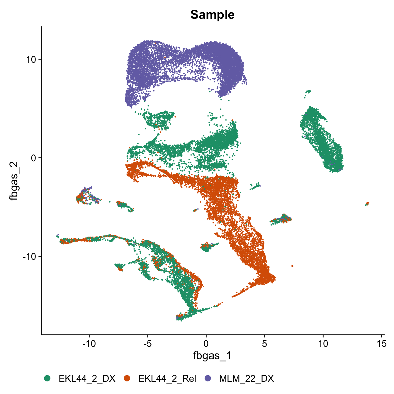
p2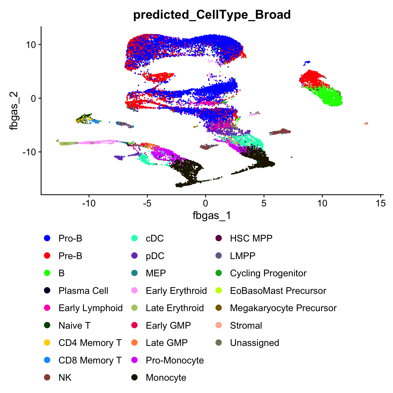
Publication-quality UMAP coloured by sample (left) and BoneMarrowMap-annotated cell type (right), using a curated colour palette that groups cell types by lineage. This two-panel plot corresponds to Figure 3A–B.
# Figure 3A-B: Combined UMAP coloured by sample and BoneMarrowMap cell type

# ── Sample rename (done here so p1/p2 are always built with post-rename labels) ─
# EKL44_2_DX is early refractory, not diagnosis — drop the misleading _DX suffix.
# sub() is idempotent: if "EKL44_2" is already present it is unchanged.
seu@meta.data[["Sample"]] <- factor(
  sub("EKL44_2_DX", "EKL44_2", as.character(seu@meta.data[["Sample"]])),
  levels = c("MLM_22_DX", "EKL44_2", "EKL44_2_Rel")
)

# ── Shared UMAP theme ─────────────────────────────────────────────────────────
umap_theme <- function() {
  theme_classic(base_size = 10) +
    theme(
      plot.title      = element_text(size = 10, face = "bold", color = "grey15",
                                     margin = margin(b = 6)),
      axis.title      = element_blank(),
      axis.text       = element_blank(),
      axis.ticks      = element_blank(),
      axis.line       = element_blank(),
      panel.grid      = element_blank(),
      panel.border    = element_blank(),
      legend.title    = element_blank(),
      legend.text     = element_text(size = 7, color = "grey20"),
      legend.key.size = unit(0.4, "lines"),
    #  aspect.ratio    = 1,
      plot.margin     = margin(4, 4, 4, 4)
    )
}

# ── Shared arrow style (used by all 4 UMAPs in Figure 3) ─────────────────────
# Defined here so the same values are available in fig3-full for panel E.
arrow_head_size <- unit(0.10, "cm")
arrow_linewidth  <- 0.35

# ── UMAP coordinate range for axis arrows ─────────────────────────────────────
umap_coords  <- as.data.frame(seu@reductions$umap@cell.embeddings)
x_range_umap <- range(umap_coords[, 1])
y_range_umap <- range(umap_coords[, 2])
arrow_len_x  <- diff(x_range_umap) * 0.08
arrow_len_y  <- diff(y_range_umap) * 0.08

umap_arrows <- list(
  geom_segment(
    aes(x    = x_range_umap[1],
        xend = x_range_umap[1] + arrow_len_x,
        y    = y_range_umap[1],
        yend = y_range_umap[1]),
    arrow       = arrow(length = arrow_head_size, type = "closed"),
    linewidth   = arrow_linewidth, color = "black", inherit.aes = FALSE
  ),
  geom_segment(
    aes(x    = x_range_umap[1],
        xend = x_range_umap[1],
        y    = y_range_umap[1],
        yend = y_range_umap[1] + arrow_len_y),
    arrow       = arrow(length = arrow_head_size, type = "closed"),
    linewidth   = arrow_linewidth, color = "black", inherit.aes = FALSE
  ),
  annotate(
    "text",
    x     = x_range_umap[1] + arrow_len_x / 2,
    y     = y_range_umap[1] - diff(y_range_umap) * 0.04,
    label = "UMAP",
    size  = 3, fontface = "italic", color = "grey30", hjust = 0.5
  )
)

# ── Sample colours ────────────────────────────────────────────────────────────
sample_colours <- c(
  "EKL44_2"     = "#1A8A9A",   # lighter teal  (early refractory)
  "EKL44_2_Rel" = "#0A4A57",   # darker teal   (relapse — same patient)
  "MLM_22_DX"   = "#C0392B"    # red
)

# ── Cell type order and colours ───────────────────────────────────────────────
# Move MEP to sit with erythroid
cell_type_order <- c(
  "Pro-B", "Pre-B", "B", "Plasma Cell",
  "Early Lymphoid", "Naive T", "CD4 Memory T", "CD8 Memory T", "NK",
  "cDC", "pDC",
  "MEP", "Early Erythroid", "Late Erythroid",  # all erythroid together
  "Early GMP", "Late GMP", "Pro-Monocyte", "Monocyte",
  "HSC MPP", "LMPP", "Cycling Progenitor",
  "EoBasoMast Precursor", "Megakaryocyte Precursor",
  "Stromal", "Unassigned"
)

cell_type_colours <- c(
  # B lineage — blues
  "Pro-B"          = "#D6EEF8",  # lightest — most primitive
  "Pre-B"          = "#89C4E1",
  "B"              = "#2E86C1",  # mature B
  "Plasma Cell"    = "#1A3A5C",  # darkest — most differentiated

  # T lineage — greens
  "Early Lymphoid" = "#D5E8D4",  # primitive
  "Naive T"        = "#82C785",
  "CD4 Memory T"   = "#2E8B57",
  "CD8 Memory T"   = "#1A5C38",
  "NK"             = "#0D3320",  # darkest

  # Myeloid — oranges/ambers
  "Early GMP"      = "#FDE8CC",  # primitive
  "Late GMP"       = "#F5B942",
  "Pro-Monocyte"   = "#E67E22",
  "Monocyte"       = "#A04000",  # most differentiated

  # Dendritic cells — purples
  "cDC"            = "#D7BDE2",
  "pDC"            = "#7D3C98",

  # Erythroid — reds/pinks
  "MEP"            = "#FADBD8",  # primitive
  "Early Erythroid"= "#E8736A",
  "Late Erythroid" = "#C0392B",

  # Progenitors — teals
  "HSC MPP"        = "#A2D9CE",  # most primitive
  "LMPP"           = "#45B39D",
  "Cycling Progenitor" = "#1A7A8A",

  # Other lineages
  "EoBasoMast Precursor" = "#F9E79F",  # yellow
  "Megakaryocyte Precursor" = "#D4AC0D",

  # Non-haematopoietic
  "Stromal"        = "#CCD1D1",  # neutral grey
  "Unassigned"     = "#EAECEE"   # lightest grey
)


# ── Apply ordered factor ──────────────────────────────────────────────────────
seu$predicted_CellType_Broad_clean <- factor(
  ifelse(is.na(seu$predicted_CellType_Broad), "Unassigned",
         as.character(seu$predicted_CellType_Broad)),
  levels = cell_type_order
)

# ── Plot 1: Sample UMAP ───────────────────────────────────────────────────────
p1 <- DimPlot(
  seu,
  reduction = "umap",
  group.by  = "Sample",
  pt.size   = 0.5,
  label     = FALSE
) +
  scale_color_manual(values = sample_colours, name = "Sample") +
  guides(colour = guide_legend(
    ncol         = 1,
    override.aes = list(size = 3)
  )) +
  labs(title = NULL) +
  umap_arrows +
  umap_theme() +
  theme(
    legend.position = "right",
    legend.title    = element_text(size = 8, face = "bold", color = "grey15")
  )
# Reduce alpha to reveal overlapping samples
p1$layers[[1]]$aes_params$alpha <- 0.6

p2 <- DimPlot(
  seu,
  reduction = "umap",
  group.by  = "predicted_CellType_Broad_clean",
  pt.size   = 0.5,
  label     = FALSE
) +
  scale_color_manual(values = cell_type_colours, name = "Cell type\n(BoneMarrowMap)") +
  guides(colour = guide_legend(
    ncol         = 1,
    override.aes = list(size = 3)
  )) +
  labs(title = NULL) +
  umap_arrows +
  umap_theme() +
  theme(
    legend.position = "right",
    legend.title    = element_text(size = 8, face = "bold", color = "grey15")
  )

# ── Combine ───────────────────────────────────────────────────────────────────
p1 + p2 +
  plot_annotation(
    title = "Transcriptional landscape of B-ALL patient samples",
    theme = theme(
      plot.title = element_text(size = 11, face = "bold",
                                color = "grey15", hjust = 0.5)
    )
  ) +
  plot_layout(widths = c(1, 1))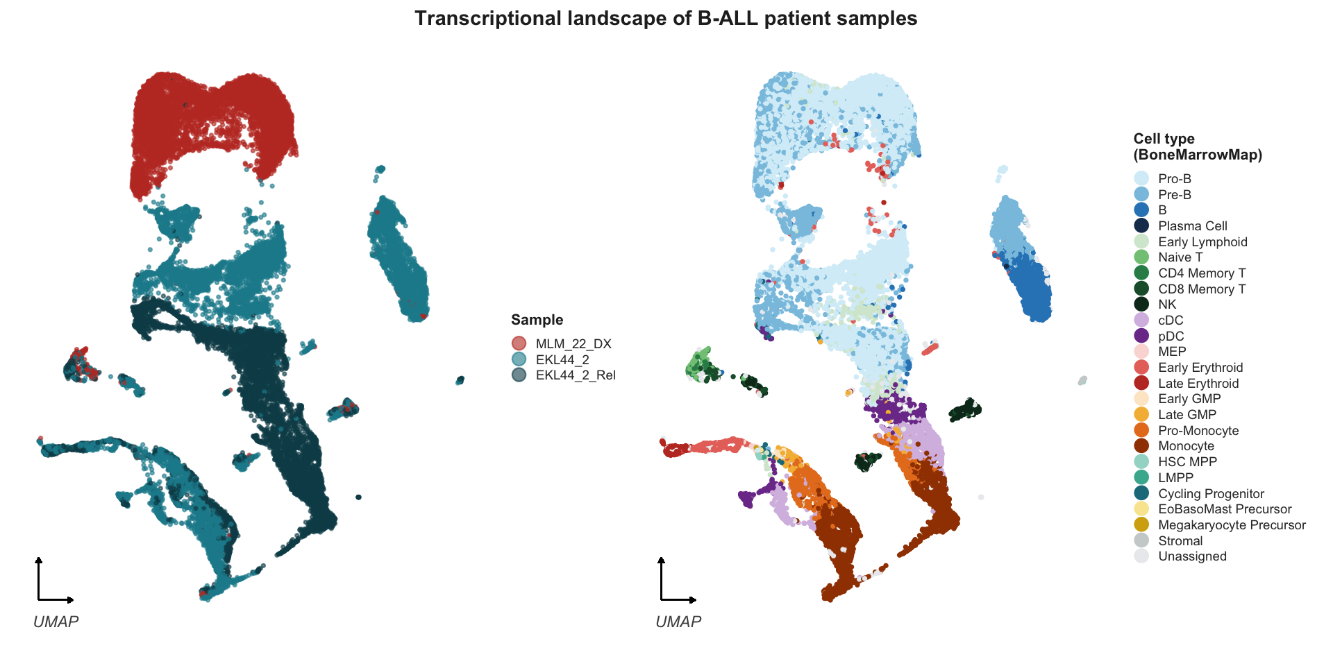
Unsupervised clustering
Each patient sample is clustered independently using SCTransform normalisation followed by Leiden clustering across a range of resolutions. This allows identification of the leukaemic cell population within each sample without interference from batch effects.
out <- here("data", "RDS", "ball_exp1_clustered.seu.rds")

if(!file.exists(out)) {

  seu_lst <- SplitObject(seu, split.by = "Sample")

  lapply(seu_lst, function(seu){
    seu <- SCTransform(seu, verbose = FALSE,
                       return.only.var.genes = FALSE)
    seu <- RunPCA(seu, verbose = FALSE, npcs = 30)
    seu <- RunUMAP(seu, dims = 1:30, reduction = "pca")

    seu <- FindNeighbors(seu, reduction = "pca", dims = 1:30)
    seu <- FindClusters(seu, resolution = seq(0.1, 1, by = 0.1),
                        algorithm = "Leiden")
    seu

  }) -> seu_lst

  saveRDS(seu_lst, file = out)
  fs::file_chmod(out, "664")
  try(fs::file_chown(out, group_id = "oshlack_lab"),
      silent = TRUE)

} else {
  seu_lst <- readRDS(out)

}
Select clustering resolution
Clustree plots show cluster stability across resolutions. Resolution 0.4 is selected as a reasonable balance between over- and under-clustering across all three samples.
lapply(seu_lst, function(seu){
  clustree(seu, prefix = "SCT_snn_res.")
})
$EKL44_2_DX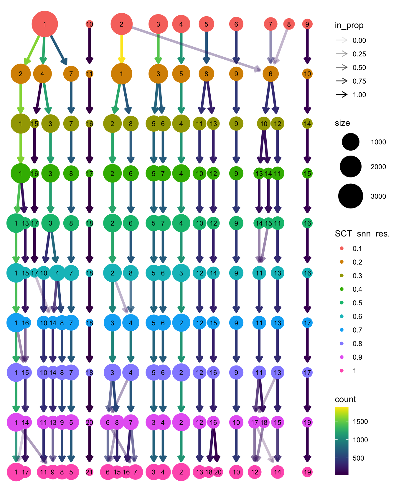
$EKL44_2_Rel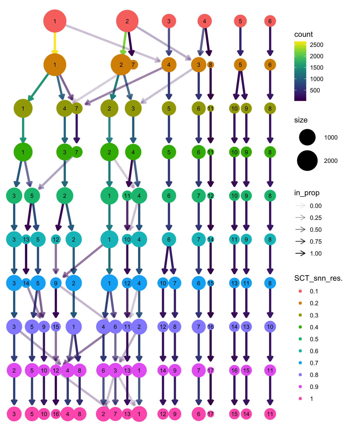
$MLM_22_DX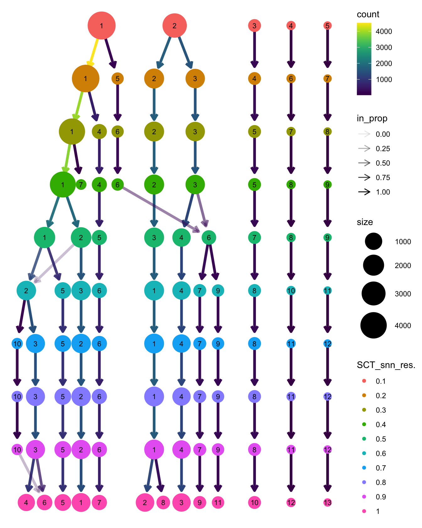
Cell cycle annotation
Cell cycle phase (S, G2M, or G1) is scored for each cell using canonical S- and G2M-phase marker gene lists from Seurat. This annotation is used to assess whether proliferating cells confound the clustering structure.
s.genes <- cc.genes$s.genes
g2m.genes <- cc.genes$g2m.genes

lapply(seu_lst, function(seu){
  seu <- CellCycleScoring(seu,
                          s.features = s.genes,
                          g2m.features = g2m.genes)
  seu
}) -> seu_lst
Cluster UMAPs
Exploratory per-sample UMAPs showing unsupervised clusters, fusion-positive cells highlighted, BoneMarrowMap cell type labels, and cell cycle phase.
grp <- rep("SCT_snn_res.0.4", length(seu_lst))

lapply(seq_along(1:length(grp)), function(i){
  DimPlot(seu_lst[[i]], reduction = "umap", label = TRUE, repel = TRUE,
          label.size = 2.5, group.by = grp[i]) +
    theme(legend.text = element_text(size = 8)) -> p1

    DimPlot(seu_lst[[i]], reduction = "umap", label = TRUE, repel = TRUE,
          label.size = 2.5, group.by = grp[i],
          cells.highlight = which(seu_lst[[i]]$patient_fusion != "not-detected")) +
    NoLegend() -> p2

    DimPlot(seu_lst[[i]], reduction = "umap", label = TRUE, repel = TRUE,
          label.size = 2.5, group.by = "predicted_CellType_Broad") +
    NoLegend() -> p3

    DimPlot(seu_lst[[i]], reduction = "umap", label = TRUE, repel = TRUE,
          label.size = 2.5, group.by = "Phase") +
    NoLegend() -> p4

  wrap_plots(p1, p2, p3, p4) + plot_annotation(title = names(seu_lst)[i])
}) -> p

p
[[1]]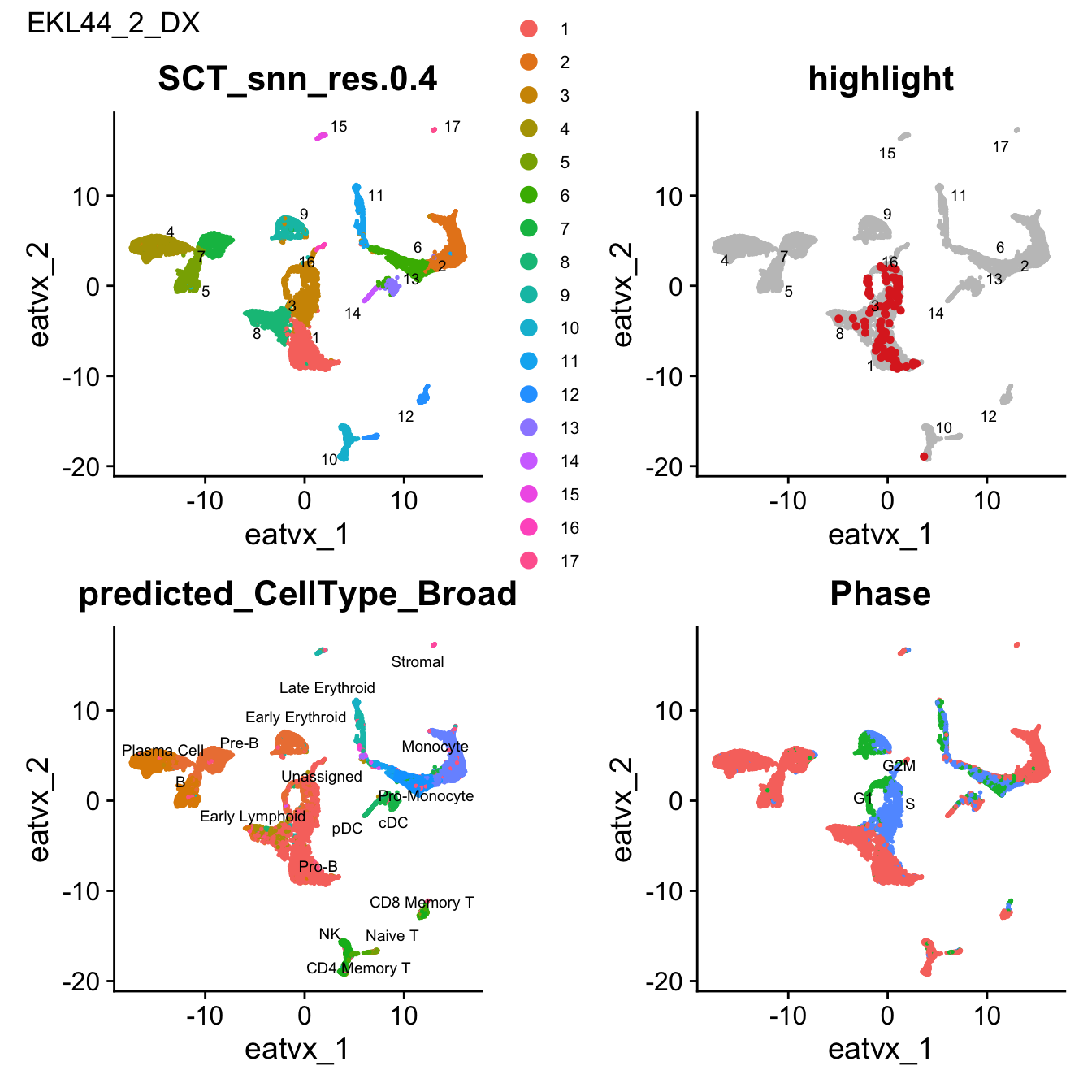
[[2]]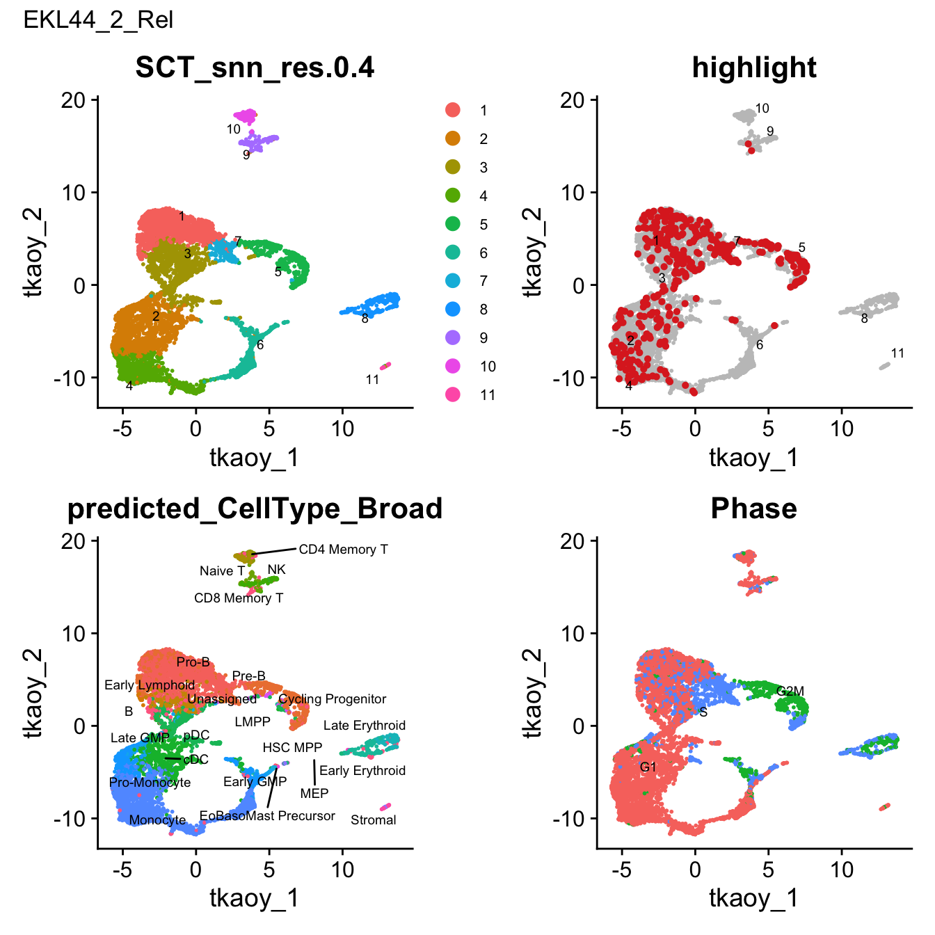
[[3]]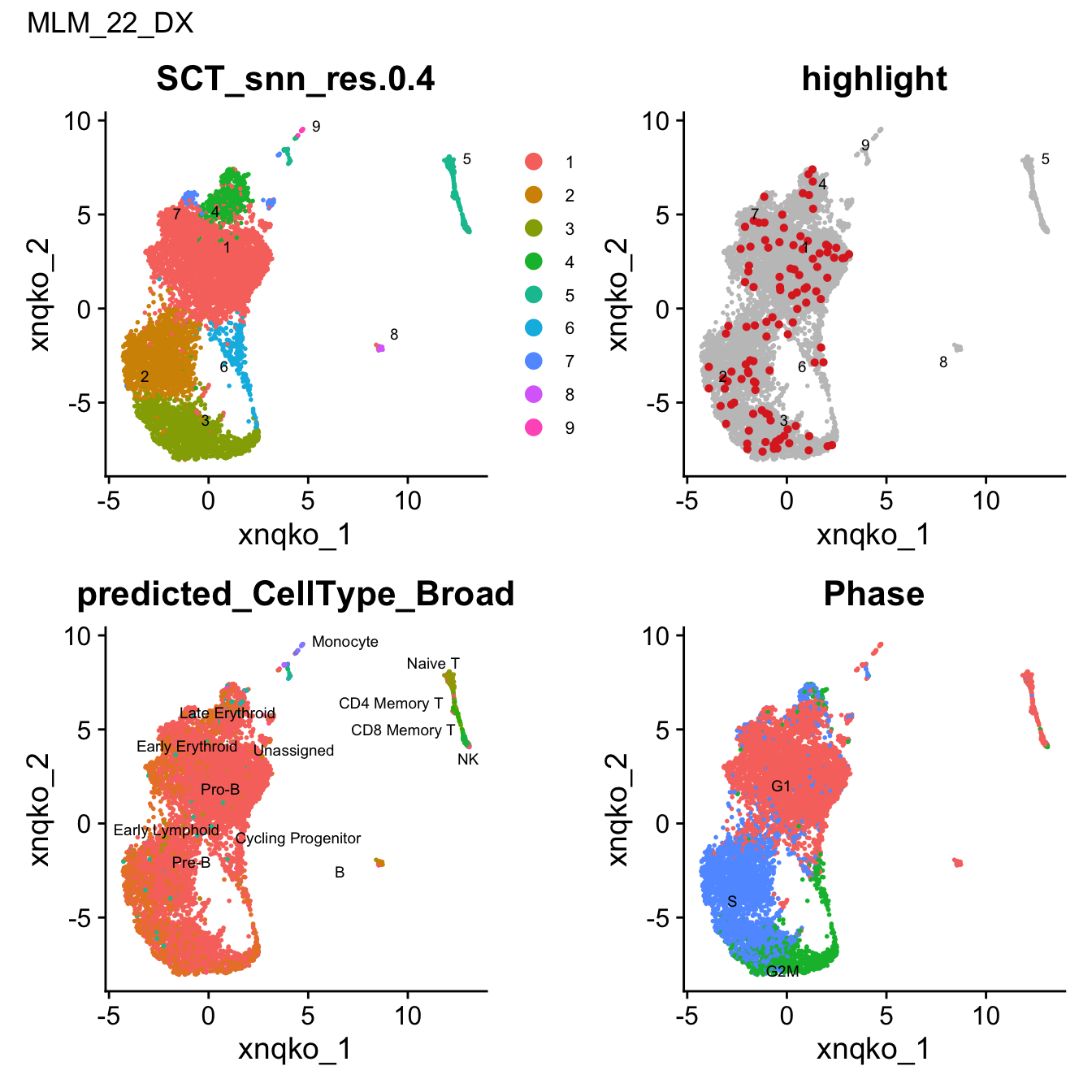
Comparing EKL44_2 at diagnosis and relapse reveals transcriptionally distinct clusters at diagnosis (e.g. Pro-B and monocyte-like populations) that become more similar at relapse, coinciding with an expansion of fusion-expressing cells with a monocyte-like transcriptional profile.
Publication-quality per-sample figure showing, for each of the three patient samples (rows): unsupervised cluster labels, majority-vote cell type annotation, fusion transcript expression highlighted per fusion type, and a dot plot of canonical lineage markers. Rows are ordered MLM_22_DX → EKL44_2 → EKL44_2_Rel (the middle sample is internally keyed as “EKL44_2_DX” — early refractory, not diagnosis — but displayed as “EKL44_2”; see the display-name relabel below). This figure contributes to Figure 3C and Figure 3E, and forms panel C of Supplementary Figure 2 (assembled with the QC summary panels below).
# Figure 3C, 3E / Supplementary Figure 2C: Per-sample four-panel figure
# ── Shared theme for all panels ───────────────────────────────────────────────
umap_theme_supp <- function() {
  theme_classic(base_size = 11) +
    theme(
      plot.title       = element_text(size = 11, face = "bold", color = "grey15",
                                      hjust = 0.5, margin = margin(b = 4)),
      axis.title       = element_blank(),
      axis.text        = element_blank(),
      axis.ticks       = element_blank(),
      axis.line        = element_blank(),
      panel.grid       = element_blank(),
      panel.border     = element_blank(),
      legend.text      = element_text(size = 9, color = "grey20"),
      legend.key.size  = unit(0.5, "lines"),
      legend.title     = element_blank(),
      plot.margin      = margin(8, 2, 8, 2)
    )
}

dot_theme_supp <- function() {
  theme_classic(base_size = 9) +
    theme(
      plot.title       = element_text(size = 11, face = "bold", color = "grey15",
                                      hjust = 0.5, margin = margin(b = 4)),
      axis.text.x      = element_text(size = 6, color = "grey20",
                                      angle = 90, hjust = 1, vjust = 0.5),
      axis.text.y      = element_text(size = 7, color = "grey15"),
      axis.title       = element_blank(),
      panel.grid.major = element_line(color = "grey92", linewidth = 0.3),
      legend.text      = element_text(size = 7, color = "grey20"),
      legend.key.size  = unit(0.4, "lines"),
      legend.title     = element_text(size = 7, color = "grey20"),
      plot.margin      = margin(8, 2, 8, 2)
    )
}

# ── Sample order ──────────────────────────────────────────────────────────────
sample_order <- c("MLM_22_DX", "EKL44_2_DX", "EKL44_2_Rel")
seu_lst      <- seu_lst[sample_order]

# ── Fusion colours ────────────────────────────────────────────────────────────
fusion_colours <- c(
  "P2RY8::CRLF2"   = "#E69F00",
  "NR3C1::ZSCAN26" = "#CC79A7",
  "BRD9::NUTM1"    = "#009E73"
)

# ── Canonical markers ─────────────────────────────────────────────────────────
# CD19 (B), CD3E (T), and CD14 (monocyte) are broad lineage markers relevant
# to every sample — all three patients have these populations. CD34 (HSC/
# progenitor) was dropped: a diagnostic check (see B-ALL_exp1_clustering
# session notes) showed CD34 is genuinely high in HSC MPP/LMPP/Cycling
# Progenitor/Early GMP/MEP cells, but those populations are only 1-37 cells
# per sample — far too rare to ever be a cluster's majority-vote cell type
# here, so they never appear as a column in this panel. CD34 was therefore
# always going to look uniformly faint in the cell types that do appear
# (Pro-B/Pre-B/B/Monocyte etc, where it's genuinely low), which isn't
# validating anything and was also pulling down the shared colour-scale cap.
#
# Every marker below targets a single specific cell type and is
# lineage-restricted the same way HBB/CXCL12 originally were: not every
# sample has that cell type annotated at all (e.g. MLM_22_DX has no NK, DC,
# Early Erythroid, or Stromal cluster). Showing a marker in a sample with no
# matching cluster isn't validating anything — any non-zero signal there is
# most likely low-level ambient contamination, not a real population — and it
# adds a spurious, often disproportionately high value that distorts the
# shared colour scale for no biological payoff. So each of these is only
# included in a given row if its target cell type is actually present in that
# sample's annotation (`predicted_CellType_Broad`/`majority_type`).
core_markers <- c("CD19", "CD3E", "CD14")
# One marker per lineage/cell type only — DNTT and MME both mark the same
# blast/B-precursor population (Pro-B/Pre-B/Early Lymphoid), so keep DNTT
# (TdT) alone as the single blast marker rather than both.
lineage_restricted_markers <- list(
  DNTT   = c("Pro-B", "Pre-B", "Early Lymphoid"),  # blast/B-precursor (TdT) — same populations Fig 3E uses
  GNLY   = c("NK"),
  LILRA4 = c("pDC"),
  FCER1A = c("cDC"),
  HBB    = c("Early Erythroid", "Late Erythroid", "MEP"),
  CXCL12 = c("Stromal")
)
canonical_markers <- c(core_markers, names(lineage_restricted_markers))

# Display order for the dot plot's marker (y) axis, grouped by lineage in the
# same sequence as cell_type_order above (B -> T/NK -> DC -> Erythroid ->
# Myeloid -> Stromal), rather than the core/lineage-restricted split used
# above just for bookkeeping.
marker_lineage_order <- c(
  "CD19", "DNTT",             # B lineage (incl. blast/precursor)
  "CD3E", "GNLY",             # T / NK
  "FCER1A", "LILRA4",         # DC: cDC, pDC (matches cell_type_order's cDC, pDC sequence)
  "HBB",                      # Erythroid
  "CD14",                     # Myeloid
  "CXCL12"                    # Stromal
)

# ── Global max expression for consistent dot plot scale ───────────────────────
# CD19/CD3E/CD14 check whether unsupervised clusters and BoneMarrowMap
# annotations agree across the populations present in every sample. Every
# lineage-restricted marker above (DNTT/GNLY/LILRA4/FCER1A/HBB/CXCL12) is
# excluded from the scale-reference calculation below: each is expected to be
# highly and near-exclusively expressed in one specific (sometimes rare) cell
# type, so any one of them would stretch the colour scale and wash out
# CD19/CD3E/CD14's contrast with each other, the same problem HBB and CXCL12
# originally caused alone.
#
# Cap at the 95th percentile of the three reference markers rather than the
# raw max — a single unusually high value would otherwise still drag the
# ceiling up and compress everything else, the same problem at smaller scale.
# scales::squish (on the colour scale below) means values above the cap still
# render as the darkest colour rather than being clipped to NA.
#
# Important: the percentile must be computed over *expressing* cells only
# (count > 0), not all cells. The first version of this cap pooled every
# cell's normalised value, including the zeros from cells that don't express
# a given lineage marker at all (the large majority, since each marker is
# lineage-restricted) — that zero-inflated distribution's 95th percentile came
# out far lower than the group-level means actually plotted in the dot plot
# (each `mean_expr` below is itself already an average restricted to
# expressing cells), so almost every dot ended up at or past the cap and the
# whole plot looked uniformly dark. Restricting the percentile calculation to
# expressing cells only puts it on the same basis as what's plotted.
scale_ref_markers <- core_markers
ref_expr_vals <- unlist(lapply(seu_lst, function(s) {
  avail  <- scale_ref_markers[scale_ref_markers %in% rownames(s)]
  counts <- GetAssayData(s, layer = "counts")[avail, , drop = FALSE]
  norm   <- GetAssayData(s, layer = "data")[avail, , drop = FALSE]
  as.numeric(norm)[as.numeric(counts) > 0]
}))
global_max_expr <- unname(quantile(ref_expr_vals, probs = 0.95, na.rm = TRUE))

# ── Column title theme ────────────────────────────────────────────────────────
col_title_theme <- theme(
  plot.title = element_text(size = 11, face = "bold", color = "grey15",
                            hjust = 0.5, margin = margin(b = 20))
)

# ── Small UMAP axis-arrow annotation, leftmost column only ────────────────────
# Each row is an independent per-sample UMAP embedding with its own coordinate
# range, so (unlike Figure 3, where all samples share one joint embedding) the
# arrows must be rebuilt per row from that row's own xlim_vals/ylim_vals.
# Reuses arrow_head_size / arrow_linewidth defined earlier (Figure 3A-B chunk)
# for a consistent look.
make_row_umap_arrows <- function(xlim_vals, ylim_vals) {
  arrow_len_x <- diff(xlim_vals) * 0.08
  arrow_len_y <- diff(ylim_vals) * 0.08
  list(
    geom_segment(
      aes(x    = xlim_vals[1],
          xend = xlim_vals[1] + arrow_len_x,
          y    = ylim_vals[1],
          yend = ylim_vals[1]),
      arrow       = arrow(length = arrow_head_size, type = "closed"),
      linewidth   = arrow_linewidth, color = "black", inherit.aes = FALSE
    ),
    geom_segment(
      aes(x    = xlim_vals[1],
          xend = xlim_vals[1],
          y    = ylim_vals[1],
          yend = ylim_vals[1] + arrow_len_y),
      arrow       = arrow(length = arrow_head_size, type = "closed"),
      linewidth   = arrow_linewidth, color = "black", inherit.aes = FALSE
    ),
    annotate(
      "text",
      x     = xlim_vals[1] + arrow_len_x / 2,
      y     = ylim_vals[1] - diff(ylim_vals) * 0.04,
      label = "UMAP",
      size  = 2.3, fontface = "italic", color = "grey30", hjust = 0.5
    )
  )
}

# ── Build panels for each sample ──────────────────────────────────────────────
all_rows <- lapply(seq_along(seu_lst), function(i) {

  s       <- seu_lst[[i]]
  s_name  <- names(seu_lst)[i]
  # Display-only relabel: EKL44_2_DX is early refractory, not diagnosis, so it
  # should read as "EKL44_2" everywhere (matching the rename already applied
  # to the joint `seu` object for Figure 3A-B). seu_lst here can come from a
  # cached ball_exp1_clustered.seu.rds (see unsupervised-clustering chunk
  # above) that may predate that rename, so the fix is applied at display time
  # rather than assumed to already be reflected in seu_lst's own names.
  s_display_name <- sub("^EKL44_2_DX$", "EKL44_2", s_name)
  is_last <- i == length(seu_lst)

  # ── Majority vote annotation per cluster ──────────────────────────────────
  cluster_annotation <- s@meta.data %>%
    tibble::rownames_to_column("cell") %>%
    mutate(
      cluster   = as.character(.data[["SCT_snn_res.0.4"]]),
      cell_type = as.character(predicted_CellType_Broad)
    ) %>%
    group_by(cluster, cell_type) %>%
    summarise(n = n(), .groups = "drop") %>%
    group_by(cluster) %>%
    slice_max(n, n = 1, with_ties = FALSE) %>%
    ungroup() %>%
    dplyr::select(cluster, majority_type = cell_type)

  s$majority_type <- cluster_annotation$majority_type[
    match(as.character(s$SCT_snn_res.0.4),
          cluster_annotation$cluster)
  ]

  # ── UMAP coordinate range ─────────────────────────────────────────────────
  umap_emb  <- Embeddings(s, reduction = "umap")
  xlim_vals <- range(umap_emb[, 1]) + c(-1, 1)
  ylim_vals <- range(umap_emb[, 2]) + c(-1, 1)
  ar        <- diff(ylim_vals) / diff(xlim_vals)

  # ── UMAP column names ─────────────────────────────────────────────────────
  umap_df   <- as.data.frame(umap_emb)
  umap_col1 <- colnames(umap_df)[1]
  umap_col2 <- colnames(umap_df)[2]

  # ── Median UMAP per majority type ─────────────────────────────────────────
  label_df <- umap_df %>%
    rownames_to_column("cell") %>%
    mutate(label = s$majority_type[cell]) %>%
    filter(!is.na(label)) %>%
    group_by(label) %>%
    summarise(
      x = median(.data[[umap_col1]]),
      y = median(.data[[umap_col2]]),
      .groups = "drop"
    )

  # ── Panel 1: Unsupervised clusters ──────────────────────────────────────────
  p1 <- DimPlot(
    s, reduction = "umap",
    group.by   = "SCT_snn_res.0.4",
    label      = TRUE, repel = TRUE,
    label.size = 2.5, pt.size = 0.4
  ) +
    labs(title = if (i == 1) "Unsupervised clusters" else NULL) +
    umap_theme_supp() +
    { if (i == 1) col_title_theme else theme() } +
    coord_cartesian(xlim = xlim_vals, ylim = ylim_vals, clip = "off") +
    make_row_umap_arrows(xlim_vals, ylim_vals) +
    theme(legend.position = "none", aspect.ratio = ar)

  # ── Panel 2: Majority vote annotation ────────────────────────────────────
  p2 <- DimPlot(
    s, reduction = "umap",
    group.by   = "majority_type",
    label      = FALSE,
    pt.size    = 0.4
  ) +
    geom_text_repel(
      data          = label_df,
      aes(x = x, y = y, label = label),
      size          = 2.5,
      color         = "grey15",
      fontface      = "plain",
      box.padding   = 0.3,
      point.padding = 0.1,
      segment.size  = 0.3,
      segment.color = "grey50",
      max.overlaps  = 20,
      inherit.aes   = FALSE
    ) +
    labs(title = if (i == 1) "Cluster annotation\n(majority vote)" else NULL) +
    umap_theme_supp() +
    { if (i == 1) col_title_theme else theme() } +
    coord_cartesian(xlim = xlim_vals, ylim = ylim_vals, clip = "off") +
    theme(legend.position = "none", aspect.ratio = ar)

  # ── Panel 3: Fusion highlight ──────────────────────────────────────────────
  # Built as a manual ggplot rather than DimPlot's cells.highlight/cols.highlight
  # (same fix as Figure 3 panels C/E): cols.highlight is paired to
  # cells.highlight positionally, and DimPlot doesn't guarantee it preserves
  # our list's order, which was rendering some samples' fusion colours
  # swapped/wrong. A named scale_colour_manual() binds colour to fusion by
  # name in the scale itself, so it can't be silently reordered.
  fusion_df3 <- umap_df %>%
    tibble::rownames_to_column("cell") %>%
    dplyr::left_join(
      tibble::rownames_to_column(s@meta.data["patient_fusion"], "cell"),
      by = "cell"
    ) %>%
    mutate(
      fusion_label = dplyr::case_when(
        patient_fusion == "P2RY8-CRLF2-fusion"   ~ "P2RY8::CRLF2",
        patient_fusion == "NR3C1-ZSCAN26-fusion"  ~ "NR3C1::ZSCAN26",
        patient_fusion == "BRD9-NUTM1-fusion"     ~ "BRD9::NUTM1",
        TRUE                                      ~ "Unselected"
      ),
      fusion_label = factor(fusion_label, levels = c("Unselected", names(fusion_colours)))
    ) %>%
    arrange(fusion_label)   # Unselected plotted first (behind fusion-positive cells)

  p3 <- ggplot(fusion_df3, aes(x = .data[[umap_col1]], y = .data[[umap_col2]],
                               colour = fusion_label)) +
    geom_point(size = 0.4, alpha = 0.8) +
    scale_colour_manual(
      values = c("Unselected" = "grey88", fusion_colours),
      breaks = names(fusion_colours),
      name   = "Fusion"
    ) +
    labs(title = if (i == 1) "Fusion expression" else NULL, x = NULL, y = NULL) +
    umap_theme_supp() +
    { if (i == 1) col_title_theme else theme() } +
    coord_cartesian(xlim = xlim_vals, ylim = ylim_vals, clip = "off") +
    # Stack the fusion-type keys vertically (one per line) rather than
    # ggplot's default horizontal row for legend.position = "bottom", which
    # was overflowing the narrow column and truncating longer fusion names.
    guides(colour = guide_legend(direction = "vertical",
                                 override.aes = list(size = 3, alpha = 1))) +
    theme(
      aspect.ratio    = ar,
      legend.position = if (is_last) "bottom" else "none",
      legend.box      = "vertical"
    )

  # ── Panel 4: Dot plot ────────────────────────────────────────────────────
  meta <- s@meta.data %>%
    tibble::rownames_to_column("cell") %>%
    mutate(majority_type = s$majority_type[cell])

  # Only include a lineage-restricted marker if its target cell type is
  # actually annotated in this sample (see lineage_restricted_markers above);
  # core lineage markers are always included. Markers are then ordered by
  # marker_lineage_order (grouped by lineage), not by core/extra membership.
  present_types <- unique(na.omit(as.character(s$majority_type)))
  extra_markers <- names(lineage_restricted_markers)[
    vapply(lineage_restricted_markers,
           function(types) any(types %in% present_types),
           logical(1))
  ]
  sample_markers <- marker_lineage_order[marker_lineage_order %in% c(core_markers, extra_markers)]
  avail_markers  <- sample_markers[sample_markers %in% rownames(s)]
  marker_counts  <- GetAssayData(s, layer = "counts")[avail_markers, ]
  marker_norm    <- GetAssayData(s, layer = "data")[avail_markers, ]

  dot_df <- lapply(avail_markers, function(gn) {
    counts_vec <- as.numeric(marker_counts[gn, meta$cell])
    norm_vec   <- as.numeric(marker_norm[gn, meta$cell])
    meta %>%
      mutate(expressed = counts_vec > 0, norm_expr = norm_vec) %>%
      group_by(majority_type) %>%
      summarise(
        pct_expressing = mean(expressed) * 100,
        mean_expr      = ifelse(any(expressed),
                                mean(norm_expr[expressed]), NA_real_),
        .groups = "drop"
      ) %>%
      mutate(marker = gn)
  }) %>%
    bind_rows() %>%
    mutate(
      marker = factor(marker, levels = rev(avail_markers)),
      # cell_type_order (defined earlier, Figure 3A-B chunk) already groups
      # cell types by lineage in the same sequence marker_lineage_order
      # follows above, so reuse it here for a consistent x-axis ordering.
      majority_type = factor(majority_type, levels = cell_type_order)
    )

  p4 <- ggplot(
    dot_df %>% filter(!is.na(pct_expressing) & pct_expressing > 0),
    aes(x = majority_type, y = marker,
        size = pct_expressing, colour = mean_expr)
  ) +
    geom_point(alpha = 0.9) +
    # Same palette as the Figure 3 Panel F marker dot plot (Purples distiller),
    # with a 95th-percentile cap (see global_max_expr above) so
    # CD19/CD3E/CD14 stay visually distinct from each other rather than
    # reading as pale near-white, while oob = squish still renders every
    # lineage-restricted marker (DNTT/GNLY/LILRA4/FCER1A/HBB/CXCL12) as the
    # darkest colour rather than washing out everything else or clipping to NA.
    # NB: an earlier version of this scale added trans = "sqrt" on top of the
    # percentile cap, which over-corrected — sqrt's steep slope near zero
    # pushed even modest expression values most of the way up the colour
    # range, so everything looked uniformly dark instead of showing gradation
    # (and produced overlapping colourbar tick labels). Removed; the
    # percentile cap alone is doing the contrast work now.
    scale_colour_distiller(
      palette   = "Purples",
      direction = 1,
      name      = "Mean\nexpr.",
      limits    = c(0, global_max_expr),
      na.value  = "grey80",
      oob       = scales::squish,
      guide     = guide_colourbar(direction    = "horizontal",
                                  title.position = "left",
                                  barwidth     = 4,
                                  barheight    = 0.5)
    ) +
    scale_size_continuous(
      name   = "% expr.",
      range  = c(0.5, 6),
      breaks = c(1, 25, 50, 75),
      limits = c(0, 100),
      guide  = guide_legend(direction = "horizontal",
                            title.position = "left",
                            nrow = 1)
    ) +
    scale_y_discrete(drop = TRUE) +
    labs(title = if (i == 1) "Marker expression\nper cell type" else NULL) +
    dot_theme_supp() +
    { if (i == 1) col_title_theme else theme() } +
    theme(
      axis.text.x     = element_text(size = 6, angle = 90,
                                     hjust = 1, vjust = 0.5),
      # Only the last row keeps its legend visible, so it sits directly under
      # the Marker expression column instead of being duplicated on every row.
      legend.position = if (is_last) "bottom" else "none",
      # legend.box (vertical) stacks the colour-bar legend above the size
      # legend instead of side by side — the two together were overflowing
      # the narrow column width. Each legend keeps its own internal
      # horizontal orientation (bar width / one row of size keys).
      legend.box = "vertical",
      legend.direction = "horizontal"
    )

  # ── Vertical sample label ─────────────────────────────────────────────────
  label_panel <- ggplot() +
    annotate(
      "text",
      x = 0.5, y = 0.5,
      label    = s_display_name,
      angle    = 90,
      size     = 4,
      fontface = "bold",
      color    = "grey15"
    ) +
    theme_void() +
    theme(plot.margin = margin(0, 6, 0, 6),
          legend.position = "none")

  # ── Assemble row ──────────────────────────────────────────────────────────
  row <- (label_panel | p1 | p2 | p3 | p4) +
    plot_layout(widths = c(0.06, 1, 1, 1, 0.5))

  row
})

# ── Stack all rows ─────────────────────────────────────────────────────────────
# No shared guide_area()/guides="collect" here: only the last row's fusion
# (p3) and marker (p4) panels have a visible legend (set via legend.position
# above), so each legend simply renders inline, directly under its own
# column, instead of being collected into one shared strip at the bottom.
p_supp2c <- wrap_plots(all_rows, ncol = 1)

p_supp2c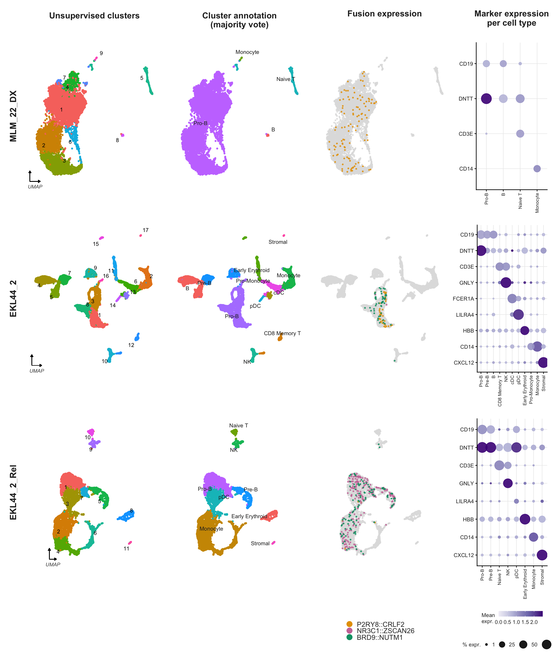
Supplementary Figure 2
Panels A–B are the QC recovery/violin summary, reusing the
four-sample (MCF7 + three B-ALL patients) QC’d object saved by
B-ALL_exp1_quality_control.Rmd. MCF7 is excluded from the
annotated Seurat object (seu) used everywhere else in this
notebook, so these two panels are the only ones that need the earlier
QC-stage object rather than seu/seu_lst. Panel
C is the per-sample clustering/annotation/fusion/marker grid
(p_supp2c) built above.
qc_sce <- readRDS(here("data", "RDS", "exp1_qc.sce.rds"))

# EKL44_2_DX is early refractory, not diagnosis — drop the misleading _DX
# suffix, matching the rename already applied to `seu` for Figure 3A-B.
# exp1_qc.sce.rds is produced independently by B-ALL_exp1_quality_control.Rmd,
# which doesn't apply this rename, so it's repeated here for panels A-B.
qc_sce$Sample <- sub("^EKL44_2_DX$", "EKL44_2", as.character(qc_sce$Sample))
# Supplementary Figure 2A-B: cell recovery + QC violins (MCF7 + 3 B-ALL samples)
supp2_sample_colours <- c(
"MCF7" = "#888888",
"MLM_22_DX" = "#56B4E9",
"EKL44_2" = "#E69F00",
"EKL44_2_Rel" = "#D55E00"
)
supp2_sample_levels <- c("MCF7", "MLM_22_DX", "EKL44_2", "EKL44_2_Rel")
# ── Panel A: Cell recovery ─────────────────────────────────────────────────────
supp2_cell_counts <- data.frame(table(qc_sce$Sample)) %>%
setNames(c("Sample", "n_cells")) %>%
mutate(Sample = factor(Sample, levels = rev(supp2_sample_levels)))
p_supp2a <- ggplot(supp2_cell_counts,
aes(x = Sample, y = n_cells, fill = Sample)) +
geom_col(width = 0.7) +
geom_text(aes(label = n_cells),
hjust = -0.1, size = 2.8, color = "grey30") +
scale_fill_manual(values = supp2_sample_colours, guide = "none") +
scale_y_continuous(expand = expansion(mult = c(0, 0.15)),
labels = scales::comma) +
coord_flip() +
labs(x = NULL, y = "Cells retained",
title = "Cell recovery after QC") +
theme_classic(base_size = 10) +
theme(
plot.title = element_text(size = 10, face = "bold",
color = "grey15", margin = margin(b = 8)),
axis.text = element_text(size = 8, color = "grey20"),
axis.line = element_line(color = "grey60", linewidth = 0.4),
axis.ticks = element_line(color = "grey60", linewidth = 0.3),
panel.grid.major.x = element_line(color = "grey95", linewidth = 0.4)
)
# ── QC data ────────────────────────────────────────────────────────────────────
supp2_qc_df <- colData(qc_sce) %>%
data.frame() %>%
dplyr::select(Sample, sum, detected, subsets_is_mito_percent) %>%
mutate(Sample = factor(Sample, levels = supp2_sample_levels))
# ── Violin helper ──────────────────────────────────────────────────────────────
make_supp2_violin <- function(df, y_var, y_lab, log_scale = FALSE) {
p <- ggplot(df, aes(x = Sample,
y = .data[[y_var]],
fill = Sample)) +
geom_violin(scale = "width",
trim = TRUE,
linewidth = 0.3,
color = "grey30",
alpha = 0.85) +
geom_boxplot(width = 0.12,
fill = "white",
color = "grey30",
linewidth = 0.3,
outlier.shape = NA) +
scale_fill_manual(values = supp2_sample_colours, guide = "none") +
labs(x = NULL, y = y_lab) +
theme_classic(base_size = 9) +
theme(
axis.text.x = element_text(size = 7, color = "grey20",
angle = 45, hjust = 1),
axis.text.y = element_text(size = 7, color = "grey30"),
axis.title.y = element_text(size = 8, color = "grey20",
margin = margin(r = 4)),
axis.line = element_line(color = "grey60", linewidth = 0.4),
axis.ticks = element_line(color = "grey60", linewidth = 0.3),
panel.grid.major.y = element_line(color = "grey95", linewidth = 0.3)
)
if (log_scale) p <- p + scale_y_log10(labels = scales::comma)
p
}
p_supp2b1 <- make_supp2_violin(supp2_qc_df, "sum", "Total UMI (log scale)", log_scale = TRUE)
p_supp2b2 <- make_supp2_violin(supp2_qc_df, "detected", "Genes detected")
p_supp2b3 <- make_supp2_violin(supp2_qc_df, "subsets_is_mito_percent", "Mitochondrial %")
# Panels A and B sit side by side as the top row (C goes full-width below,
# not beside them, so A and B share the row instead of stacking in a column).
p_supp2ab <- p_supp2a + (p_supp2b1 / p_supp2b2 / p_supp2b3) +
plot_layout(ncol = 2, widths = c(1, 1))
p_supp2ab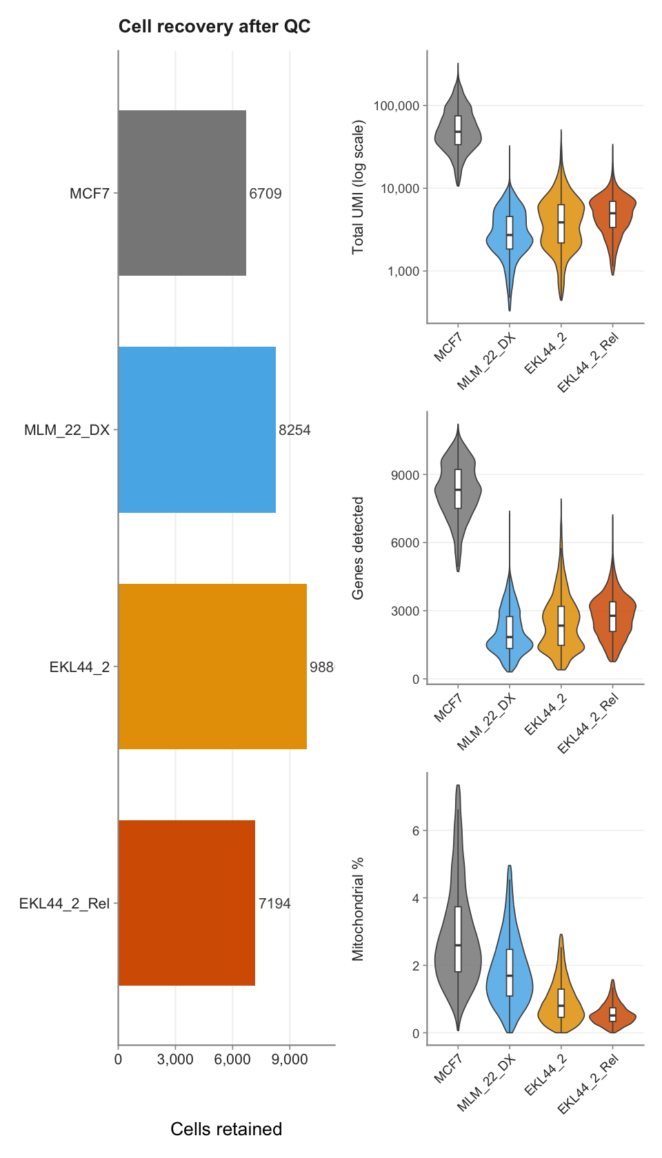
Assemble Supplementary Figure 2
Panels A–B (QC summary, side by side) form the top row; panel C
(per-sample clustering grid, p_supp2c, built above) spans
the full width beneath. There is no separate panel for fusion/marker
expression restricted to EKL44_2 diagnosis vs. relapse — that dot plot
(previously mislabelled “Supplementary Figure 3A” in
B-ALL_exp1_annotate_with_BoneMarrowMap.Rmd) has been
dropped as redundant with panel C, which already shows marker expression
per cell type for every sample including both EKL44_2 timepoints.
Figure 3’s exact tagging mechanism (flat + combination
of panels each carrying their own + tag_theme, then
plot_annotation(tag_levels = "A")) doesn’t transfer
directly here, and the previous render confirms why: every one of Figure
3’s six panels (p1/p2/pC/pD/pE/pF) is a single leaf ggplot (pE achieves
its per-sample look with facet/split.by, not
patchwork nesting), so patchwork tags each of the six once. Panel B (the
violin stack) and panel C (the per-sample grid) here are themselves
nested patchwork compositions built from many leaf ggplots —
combining them with a bare + exposes every one of those
leaves to plot_annotation(), which is why the previous
attempt produced tags A through S instead of A/B/C (one tag per leaf
panel, not per conceptual panel).
wrap_elements() is the fix for tag
placement/scope: it converts a whole nested composition into a
single opaque patch, so patchwork’s tagging treats it as one panel
again. But theming the content before it gets wrapped doesn’t
work either way (tried both + and & —
neither reaches the tag). wrap_elements() doesn’t inspect
the theme of what it’s given; it treats the input as generic graphics
and renders the tag using its own patch-level theme. That theme lives on
the object wrap_elements() returns, so styling has
to be applied to that returned patch, after wrapping — the same
+ tag_theme idiom Figure 3 uses, just applied one level
further out (to the wrapped patch, not the pre-wrap ggplot).
# Supplementary Figure 2: full assembly with A/B/C plot tags (size 18, bold,
# matching Figure 3's tag styling). wrap_elements() makes the violin stack
# (B) and per-sample grid (C) each count as a single taggable panel instead
# of patchwork descending into and tagging every leaf plot inside them.
tag_theme <- theme(plot.tag = element_text(size = 18, face = "bold"))

# Panel B gets its own title (Panel A already has one) so the top row reads
# as two clearly labelled panels rather than one titled + one bare.
supp2_violins <- (p_supp2b1 / p_supp2b2 / p_supp2b3) +
  plot_annotation(title = "QC metrics per sample",
                  theme = theme(plot.title = element_text(
                    size = 10, face = "bold", color = "grey15",
                    margin = margin(b = 8))))

# Apply tag_theme to the wrap_elements() *output*, not the pre-wrap content —
# that output is the actual patch patchwork tags, so its theme is what
# controls tag styling. (Theming the content before wrapping, tried with
# both `+` and `&`, doesn't propagate through — wrap_elements() doesn't
# inspect the theme of what's handed to it.)
pA_tagged <- wrap_elements(p_supp2a) + tag_theme
pB_tagged <- wrap_elements(supp2_violins) + tag_theme
pC_tagged <- wrap_elements(p_supp2c) + tag_theme

supp2_design <- "
AABB
CCCC
"

pA_tagged + pB_tagged + pC_tagged +
  plot_layout(design = supp2_design, heights = c(0.4, 1)) +
  plot_annotation(tag_levels = "A")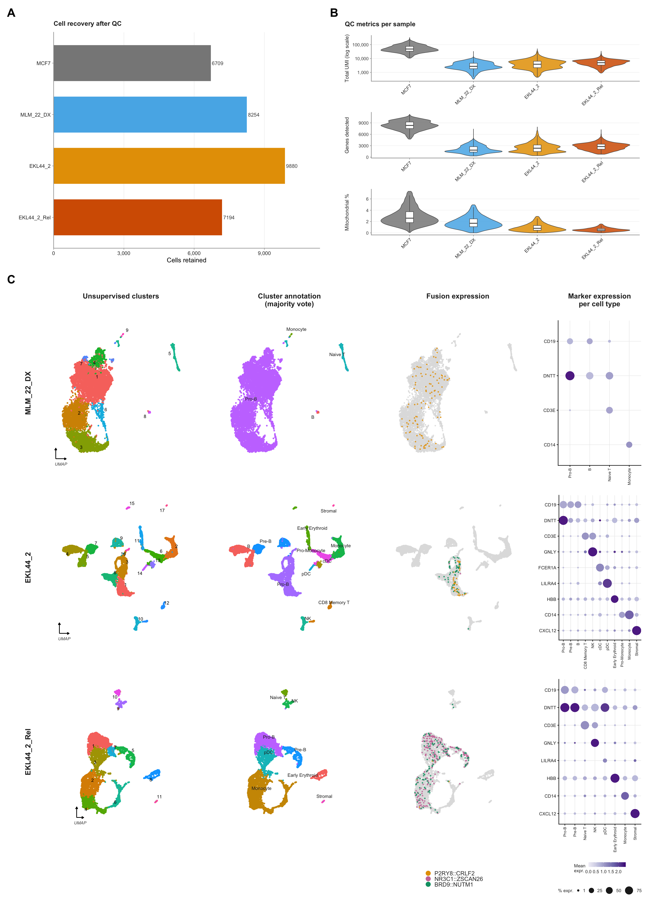
Supplementary Figure 2. Quality control and per-sample clustering for B-ALL Experiment 1. (A) Cells retained per sample after QC filtering. (B) Violin plots of total UMI count (log scale), genes detected, and mitochondrial read percentage per sample after filtering. (C) Per-sample unsupervised Leiden clustering (SCT normalisation, resolution = 0.4; left column), with cluster identities assigned by majority vote of BoneMarrowMap broad cell type annotations (centre-left column). Fusion-positive cells are highlighted per sample (centre-right column). Canonical lineage marker expression per majority-annotated cell type confirms concordance between unsupervised clusters and BoneMarrowMap annotations (right column); marker expression is shown as mean normalised expression (colour) and percentage of cells expressing (dot size).
Figure 3
Panels A and B are defined above (p1 and
p2). Panels C–F are built here using the annotated Seurat
object, then all six are assembled as a single patchwork figure.
- A Joint UMAP coloured by sample
- B Joint UMAP coloured by BoneMarrowMap broad cell type
- C Joint UMAP with fusion-positive cells highlighted
- D Bar chart: fusion-positive cell counts per sample
- E Per-sample BoneMarrowMap UMAPs with fusion highlights and cell type labels
- F Marker dot plot across fusion+/− cell groups per sample
# ── Shared fusion colours ──────────────────────────────────────────────────────
fusion_colours <- c(
  "P2RY8::CRLF2"   = "#E69F00",
  "NR3C1::ZSCAN26" = "#CC79A7",
  "BRD9::NUTM1"    = "#009E73"
)

# ── Override p1/p2 legend position for fig3 (bottom saves horizontal space) ───
# Rename is done upstream in fig-exp1-sample-celltype-umap; p1 already has
# "EKL44_2" labels. sample_colours is also defined there.
p1 <- p1 +
  labs(title = "Sample") +
  scale_color_manual(
    values = sample_colours,
    name   = "Sample"
  ) +
  guides(colour = guide_legend(ncol = 3, title.position = "top",
                               override.aes = list(size = 3))) +
  theme(legend.position      = "bottom",
        legend.justification = "top",
        plot.title           = element_text(size = 10, face = "bold", color = "grey15",
                                            margin = margin(b = 4)),
        legend.title         = element_text(size = 8, face = "bold", color = "grey15"))
p2 <- p2 +
  labs(title = "Cell type") +
  guides(colour = guide_legend(ncol = 3, title.position = "top",
                               override.aes = list(size = 3))) +
  theme(legend.position      = "bottom",
        legend.justification = "top",
        plot.title           = element_text(size = 10, face = "bold", color = "grey15",
                                            margin = margin(b = 4)),
        legend.title         = element_text(size = 8, face = "bold", color = "grey15"))

# ══════════════════════════════════════════════════════════════════════════════
# Panel C: fusion-positive cells on the joint normalised UMAP
# ══════════════════════════════════════════════════════════════════════════════
# Rebuilt directly from seu (joined by barcode) rather than reusing the
# umap_coords object captured much earlier in fig-exp1-sample-celltype-umap:
# a positional mutate() of seu$patient_fusion onto that old data frame is only
# correct if cell order in seu never shifted between the two chunks, and in
# this consolidated notebook it's not safe to assume that. Joining by barcode
# guarantees each cell's coordinates and fusion status stay paired correctly
# regardless of any reordering in between.
plot_df_c <- as.data.frame(seu@reductions$umap@cell.embeddings) %>%
  setNames(c("UMAP_1", "UMAP_2")) %>%
  tibble::rownames_to_column("barcode") %>%
  dplyr::left_join(
    tibble::rownames_to_column(seu@meta.data["patient_fusion"], "barcode"),
    by = "barcode"
  ) %>%
  mutate(
    fusion_label = dplyr::case_when(
      patient_fusion == "P2RY8-CRLF2-fusion"   ~ "P2RY8::CRLF2",
      patient_fusion == "NR3C1-ZSCAN26-fusion"  ~ "NR3C1::ZSCAN26",
      patient_fusion == "BRD9-NUTM1-fusion"     ~ "BRD9::NUTM1",
      TRUE                                      ~ "Unselected"
    ),
    fusion_label = factor(fusion_label, levels = c("Unselected", names(fusion_colours)))
  ) %>%
  arrange(fusion_label)   # Unselected plotted first (behind fusion-positive cells)

pC <- ggplot(plot_df_c, aes(x = UMAP_1, y = UMAP_2, colour = fusion_label)) +
  geom_point(size = 0.5, alpha = 0.8) +
  scale_colour_manual(
    values = c("Unselected" = "grey88", fusion_colours),
    breaks = names(fusion_colours),
    name   = "Fusion"
  ) +
  guides(colour = guide_legend(ncol = 3, title.position = "top",
                               override.aes = list(size = 3, alpha = 1))) +
  labs(title = "Fusion detection") +
  umap_arrows +
  umap_theme() +
  theme(
    plot.title           = element_text(size = 10, face = "bold", color = "grey15",
                                        margin = margin(b = 4)),
    legend.position      = "bottom",
    legend.justification = "top",
    legend.title         = element_text(size = 8, face = "bold", color = "grey15"),
    legend.text          = element_text(size = 7, color = "grey20")
  )

# ══════════════════════════════════════════════════════════════════════════════
# Panel D: fusion-positive cell counts per sample
# ══════════════════════════════════════════════════════════════════════════════
fusion_sample_counts <- seu@meta.data %>%
  filter(patient_fusion != "not-detected") %>%
  mutate(
    fusion_label = dplyr::case_when(
      patient_fusion == "P2RY8-CRLF2-fusion"   ~ "P2RY8::CRLF2",
      patient_fusion == "NR3C1-ZSCAN26-fusion"  ~ "NR3C1::ZSCAN26",
      patient_fusion == "BRD9-NUTM1-fusion"     ~ "BRD9::NUTM1",
      TRUE                                      ~ patient_fusion
    )
  ) %>%
  group_by(Sample, fusion_label) %>%
  summarise(n_cells = n(), .groups = "drop") %>%
  complete(
    Sample       = levels(seu$Sample),
    fusion_label = names(fusion_colours),
    fill         = list(n_cells = 0)
  ) %>%
  mutate(
    Sample       = factor(Sample, levels = levels(seu$Sample)),
    fusion_label = factor(fusion_label, levels = names(fusion_colours))
  )

pD <- ggplot(fusion_sample_counts,
             aes(x = Sample, y = n_cells, fill = fusion_label)) +
  geom_col(position = position_dodge(width = 0.75),
           width     = 0.65,
           color     = "white",
           linewidth = 0.3) +
  geom_text(
    aes(label = n_cells, y = n_cells),
    position = position_dodge(width = 0.75),
    vjust    = -0.4,
    size     = 2.8,
    color    = "grey30",
    fontface = "bold"
  ) +
  scale_fill_manual(values = fusion_colours, name = "Fusion") +
  scale_x_discrete(expand = expansion(add = 0.5)) +
  guides(fill = guide_legend(title.position = "top", nrow = 1)) +
  labs(x = NULL, y = "No. fusion-positive cells",
       title = "Fusion-positive cells") +
  theme_classic(base_size = 10) +
  theme(
    plot.title         = element_text(size = 10, face = "bold", color = "grey15",
                                      margin = margin(b = 4)),
    axis.title.y       = element_text(size = 9, color = "grey20", margin = margin(r = 4)),
    axis.text.x        = element_text(size = 8, color = "grey20"),
    axis.text.y        = element_text(size = 8, color = "grey30"),
    axis.line          = element_line(color = "grey60", linewidth = 0.4),
    axis.ticks         = element_line(color = "grey60", linewidth = 0.3),
    panel.grid.major.y = element_line(color = "grey95", linewidth = 0.4),
    legend.position      = "bottom",
    legend.justification = "top",
    legend.direction     = "horizontal",
    legend.title         = element_text(size = 8, face = "bold", color = "grey15"),
    legend.text          = element_text(size = 9, color = "grey20"),
    legend.key.size      = unit(0.4, "lines"),
    plot.margin          = margin(6, 6, 6, 6)
  )

# ══════════════════════════════════════════════════════════════════════════════
# Panel E: per-sample BoneMarrowMap UMAPs with fusion highlights + cell type labels
# ══════════════════════════════════════════════════════════════════════════════

# NA_character_ for Unassigned/NA cells — avoids a stray "NA" cell-type label
seu$predicted_CellType_Broad_plot <- dplyr::case_when(
  is.na(seu$predicted_CellType_Broad)          ~ NA_character_,
  seu$predicted_CellType_Broad == "Unassigned" ~ NA_character_,
  TRUE                                         ~ as.character(seu$predicted_CellType_Broad)
)

# Projected UMAP coordinates and arrow geometry
umap_proj_coords <- as.data.frame(seu@reductions$umap_projected@cell.embeddings)
x_range_proj     <- range(umap_proj_coords[, 1])
y_range_proj     <- range(umap_proj_coords[, 2])
arrow_len_x_proj <- diff(x_range_proj) * 0.08
arrow_len_y_proj <- diff(y_range_proj) * 0.08
arrow_y_proj     <- y_range_proj[1] - 2.5
arrow_x_proj     <- x_range_proj[1]

# Built as a manual ggplot rather than DimPlot's cells.highlight/cols.highlight
# (same fix as panel C): cols.highlight is paired to cells.highlight
# positionally, and DimPlot doesn't guarantee it preserves our list's order —
# that's what was rendering P2RY8::CRLF2/BRD9::NUTM1 swapped here. A named
# scale_colour_manual() binds colour to fusion by name in the scale itself,
# joined to coordinates by barcode so cell identity can't drift either.
plot_df_e <- as.data.frame(seu@reductions$umap_projected@cell.embeddings) %>%
  setNames(c("UMAP_1", "UMAP_2")) %>%
  tibble::rownames_to_column("barcode") %>%
  dplyr::left_join(
    seu@meta.data %>%
      tibble::rownames_to_column("barcode") %>%
      dplyr::select(barcode, patient_fusion, Sample),
    by = "barcode"
  ) %>%
  mutate(
    fusion_label = dplyr::case_when(
      patient_fusion == "P2RY8-CRLF2-fusion"   ~ "P2RY8::CRLF2",
      patient_fusion == "NR3C1-ZSCAN26-fusion"  ~ "NR3C1::ZSCAN26",
      patient_fusion == "BRD9-NUTM1-fusion"     ~ "BRD9::NUTM1",
      TRUE                                      ~ "Unselected"
    ),
    fusion_label = factor(fusion_label, levels = c("Unselected", names(fusion_colours))),
    Sample       = factor(Sample, levels = levels(seu$Sample))
  ) %>%
  arrange(fusion_label)   # Unselected plotted first (behind fusion-positive cells)

# Manual cell type label positions (median UMAP coord per type per sample)
label_df_e <- umap_proj_coords %>%
  setNames(c("UMAP_1", "UMAP_2")) %>%
  mutate(
    cell_type = seu$predicted_CellType_Broad_plot,
    Sample    = seu$Sample
  ) %>%
  filter(!is.na(cell_type), !is.na(Sample)) %>%
  group_by(Sample, cell_type) %>%
  summarise(x = median(UMAP_1), y = median(UMAP_2), .groups = "drop") %>%
  mutate(Sample = factor(Sample, levels = levels(seu$Sample)))

pE <- ggplot(plot_df_e, aes(x = UMAP_1, y = UMAP_2, colour = fusion_label)) +
  geom_point(size = 0.4, alpha = 0.8) +
  facet_wrap(~ Sample, nrow = 1) +
  scale_colour_manual(
    values = c("Unselected" = "grey85", fusion_colours),
    breaks = names(fusion_colours),
    name   = "Fusion"
  ) +
  # Cell type labels — one per type per sample, repelled from points
  geom_text_repel(
    data               = label_df_e,
    aes(x = x, y = y, label = cell_type),
    size               = 2.2,
    color              = "grey15",
    box.padding        = 0.2,
    point.padding      = 0.1,
    segment.size       = 0.25,
    segment.color      = "grey50",
    min.segment.length = 0.1,
    max.overlaps       = 25,
    inherit.aes        = FALSE
  ) +
  # Horizontal axis arrow — first sample panel only
  geom_segment(
    data = data.frame(Sample = factor(levels(seu$Sample)[1], levels = levels(seu$Sample))),
    aes(x    = arrow_x_proj,
        xend = arrow_x_proj + arrow_len_x_proj,
        y    = arrow_y_proj,
        yend = arrow_y_proj),
    arrow       = arrow(length = arrow_head_size, type = "closed"),
    linewidth   = arrow_linewidth, color = "black", inherit.aes = FALSE
  ) +
  # Vertical axis arrow — first sample panel only
  geom_segment(
    data = data.frame(Sample = factor(levels(seu$Sample)[1], levels = levels(seu$Sample))),
    aes(x    = arrow_x_proj,
        xend = arrow_x_proj,
        y    = arrow_y_proj,
        yend = arrow_y_proj + arrow_len_y_proj),
    arrow       = arrow(length = arrow_head_size, type = "closed"),
    linewidth   = arrow_linewidth, color = "black", inherit.aes = FALSE
  ) +
  # UMAP text label — first sample panel only
  geom_text(
    data = data.frame(
      Sample = factor(levels(seu$Sample)[1], levels = levels(seu$Sample)),
      x      = arrow_x_proj + arrow_len_x_proj / 2,
      y      = arrow_y_proj - diff(y_range_proj) * 0.03
    ),
    aes(x = x, y = y, label = "UMAP"),
    size        = 3,
    fontface    = "italic",
    color       = "grey30",
    hjust       = 0.5,
    inherit.aes = FALSE
  ) +
  guides(colour = guide_legend(title.position = "top", override.aes = list(size = 3, alpha = 1))) +
  labs(title = "Per-sample fusion detection and mapping to BoneMarrowMap reference",
       colour = "Fusion") +
  theme_classic(base_size = 10) +
  theme(
    plot.title       = element_text(size = 10, face = "bold", color = "grey15",
                                    margin = margin(b = 4)),
    axis.title       = element_blank(),
    axis.text        = element_blank(),
    axis.ticks       = element_blank(),
    axis.line        = element_blank(),
    panel.grid       = element_blank(),
    panel.border     = element_blank(),
    panel.spacing    = unit(1.5, "lines"),
    strip.text       = element_text(size = 10, face = "bold", color = "grey15"),
    strip.background = element_blank(),
    legend.position  = "bottom",
    legend.title     = element_text(size = 8, face = "bold", color = "grey15"),
    legend.text      = element_text(size = 8, color = "grey20"),
    legend.key.size  = unit(0.5, "lines")
  )

# ══════════════════════════════════════════════════════════════════════════════
# Panel F: marker expression dot plot across fusion+/− cell groups per sample
# ══════════════════════════════════════════════════════════════════════════════
blast_types_f <- c("Pro-B", "Pre-B", "Early Lymphoid")
myeloid_types_f <- c(
  "B", "Plasma Cell",
  "Naive T", "CD4 Memory T", "CD8 Memory T", "NK",
  "cDC", "pDC",
  "MEP", "Early Erythroid", "Late Erythroid",
  "Early GMP", "Late GMP", "Pro-Monocyte", "Monocyte",
  "HSC MPP", "LMPP", "Cycling Progenitor",
  "EoBasoMast Precursor", "Megakaryocyte Precursor",
  "Stromal"
)

seu$marker_group_f <- dplyr::case_when(
  seu$patient_fusion != "not-detected" &
    seu$predicted_CellType_Broad %in% blast_types_f              ~ "Fn+\nBlast",
  seu$Sample == "EKL44_2_Rel" &
    seu$patient_fusion != "not-detected" &
    seu$predicted_CellType_Broad %in% myeloid_types_f            ~ "Fn+\nMyeloid",
  seu$Sample == "EKL44_2_Rel" &
    seu$patient_fusion != "not-detected" &
    seu$predicted_CellType_Broad == "Unassigned"                 ~ "Fn+\nMyeloid",
  seu$patient_fusion == "not-detected" &
    seu$predicted_CellType_Broad %in% blast_types_f              ~ "Fn-\nBlast",
  seu$patient_fusion == "not-detected" &
    !seu$predicted_CellType_Broad %in% blast_types_f             ~ "Fn-\n(non-blast)",
  TRUE ~ NA_character_
)

group_levels_f <- c("Fn+\nBlast", "Fn+\nMyeloid",
                    "Fn-\nBlast", "Fn-\n(non-blast)")
# Blast/B-cell markers (top): CD19 → DNTT → MME → VPREB1 → CD34
# Myeloid markers (bottom): LYZ + CD14 (monocytic+) | MPO (granulocytic−, confirms monocytic identity)
markers_f <- c("CD19", "DNTT", "MME", "VPREB1", "CD34", "LYZ", "CD14", "MPO")

seu$marker_facet_f <- factor(seu$Sample, levels = levels(seu$Sample))

marker_counts_f <- GetAssayData(seu, layer = "counts")[markers_f, ]
marker_norm_f   <- GetAssayData(seu, layer = "data")[markers_f, ]

dot_df_f <- seu@meta.data %>%
  tibble::rownames_to_column("cell") %>%
  filter(!is.na(marker_group_f)) %>%
  dplyr::select(cell, marker_group_f, marker_facet_f) %>%
  { df <- .
    lapply(markers_f, function(gn) {
      counts_vec <- as.numeric(marker_counts_f[gn, df$cell])
      norm_vec   <- as.numeric(marker_norm_f[gn, df$cell])
      df %>%
        mutate(expressed = counts_vec > 0, norm_expr = norm_vec) %>%
        group_by(marker_group_f, marker_facet_f) %>%
        summarise(
          pct_expressing = mean(expressed) * 100,
          mean_expr      = ifelse(any(expressed), mean(norm_expr[expressed]), NA_real_),
          n              = n(),
          .groups        = "drop"
        ) %>%
        mutate(marker = gn)
    }) %>%
      bind_rows()
  } %>%
  mutate(
    marker         = factor(marker, levels = rev(markers_f)),
    marker_group_f = factor(marker_group_f, levels = group_levels_f),
    marker_facet_f = factor(marker_facet_f,
                            levels = levels(seu$Sample))
  ) %>%
  filter(!is.na(pct_expressing) | !is.na(mean_expr))

group_n_f <- seu@meta.data %>%
  filter(!is.na(marker_group_f), !is.na(marker_facet_f)) %>%
  group_by(marker_group_f, marker_facet_f) %>%
  summarise(n = n(), .groups = "drop") %>%
  mutate(
    marker_group_f = factor(marker_group_f, levels = group_levels_f),
    marker_facet_f = factor(marker_facet_f,
                            levels = levels(seu$Sample)),
    label = paste0("n=", scales::comma(n))
  )

vline_df_f <- data.frame(
  marker_facet_f = factor(levels(seu$Sample)[3], levels = levels(seu$Sample)),
  xintercept     = 2.5   # 2 Fn+ groups (Blast, Myeloid) then Fn- groups
)

pF <- ggplot(dot_df_f %>% filter(!is.na(marker_group_f)),
             aes(x = marker_group_f, y = marker,
                 size = pct_expressing, colour = mean_expr)) +
  geom_point(alpha = 0.9) +
  # Separator between myeloid markers (MPO, CD14, LYZ) and blast/B-cell markers (CD34–CD19)
  # With rev(markers_f): MPO=1, CD14=2, LYZ=3, CD34=4 → line at 3.5
  geom_hline(yintercept = 3.5, linetype = "dashed",
             colour = "grey50", linewidth = 0.4) +
  geom_text(
    data        = group_n_f,
    aes(x = marker_group_f, y = Inf, label = label),
    inherit.aes = FALSE,
    vjust       = 0.75,
    size        = 2.3,
    colour      = "grey40",
    fontface    = "italic"
  ) +
  geom_vline(
    data      = vline_df_f,
    aes(xintercept = xintercept),
    linetype  = "dashed",
    colour    = "grey60",
    linewidth = 0.4
  ) +
  facet_grid(
    cols   = vars(marker_facet_f),
    scales = "free_x",
    space  = "free_x"
  ) +
  scale_colour_distiller(
    palette   = "Purples",
    direction = 1,
    name      = "Mean\nexpr.",
    na.value  = "grey80",
    limits    = c(0, 4),         # LYZ peaks ~5.3; cap at 4 for better colour contrast
    oob       = scales::squish, # LYZ dots still show darkest purple, not NA
    guide     = guide_colourbar(direction      = "horizontal",
                                title.position = "top",
                                barwidth       = 4,
                                barheight      = 0.5)
  ) +
  scale_size_continuous(
    name   = "% expr.",
    range  = c(0.5, 8),
    breaks = c(1, 25, 50, 75),
    limits = c(0, 100),
    guide  = guide_legend(direction      = "horizontal",
                          title.position = "top",
                          nrow           = 1)
  ) +
  coord_cartesian(clip = "off") +
  labs(x = NULL, y = NULL,
       title = "Canonical marker gene expression") +
  theme_classic(base_size = 11) +
  theme(
    plot.title       = element_text(size = 10, face = "bold", colour = "grey15",
                                    hjust = 0, margin = margin(b = 6)),
    axis.text.x      = element_text(size = 7, colour = "grey15", hjust = 0.5),
    axis.text.y      = element_text(size = 9, colour = "grey15"),
    panel.grid.major = element_line(colour = "grey92", linewidth = 0.3),
    strip.background = element_blank(),
    strip.text       = element_text(size = 10, face = "bold", colour = "grey15"),
    legend.position  = "bottom",
    legend.box       = "horizontal",
    legend.direction = "horizontal",
    plot.margin      = margin(10, 6, 6, 6),
    panel.spacing    = unit(1, "lines")
  )

# ══════════════════════════════════════════════════════════════════════════════
# Assemble Figure 3  (A=p1, B=p2, C=pC, D=pD, E=pE, F=pF)
# 13-column grid: D gets 4 cols, E gets 8, F gets 5 (~54% wider than before)
# ══════════════════════════════════════════════════════════════════════════════
design <- "
AAABBBCCCDDDD
EEEEEEEEFFFFF
"

# Apply tag theme to each panel individually — & operator is unreliable across
# patchwork versions; patchwork reads plot.tag from each panel's own theme.
tag_theme <- theme(plot.tag = element_text(size = 18, face = "bold"))
p1 <- p1 + tag_theme
p2 <- p2 + tag_theme
pC <- pC + tag_theme
pD <- pD + tag_theme
pE <- pE + tag_theme
pF <- pF + tag_theme

p1 + p2 + pC + pD + pE + pF +
  plot_layout(design = design, guides = "keep", heights = c(1.1, 1)) +
  plot_annotation(tag_levels = "A")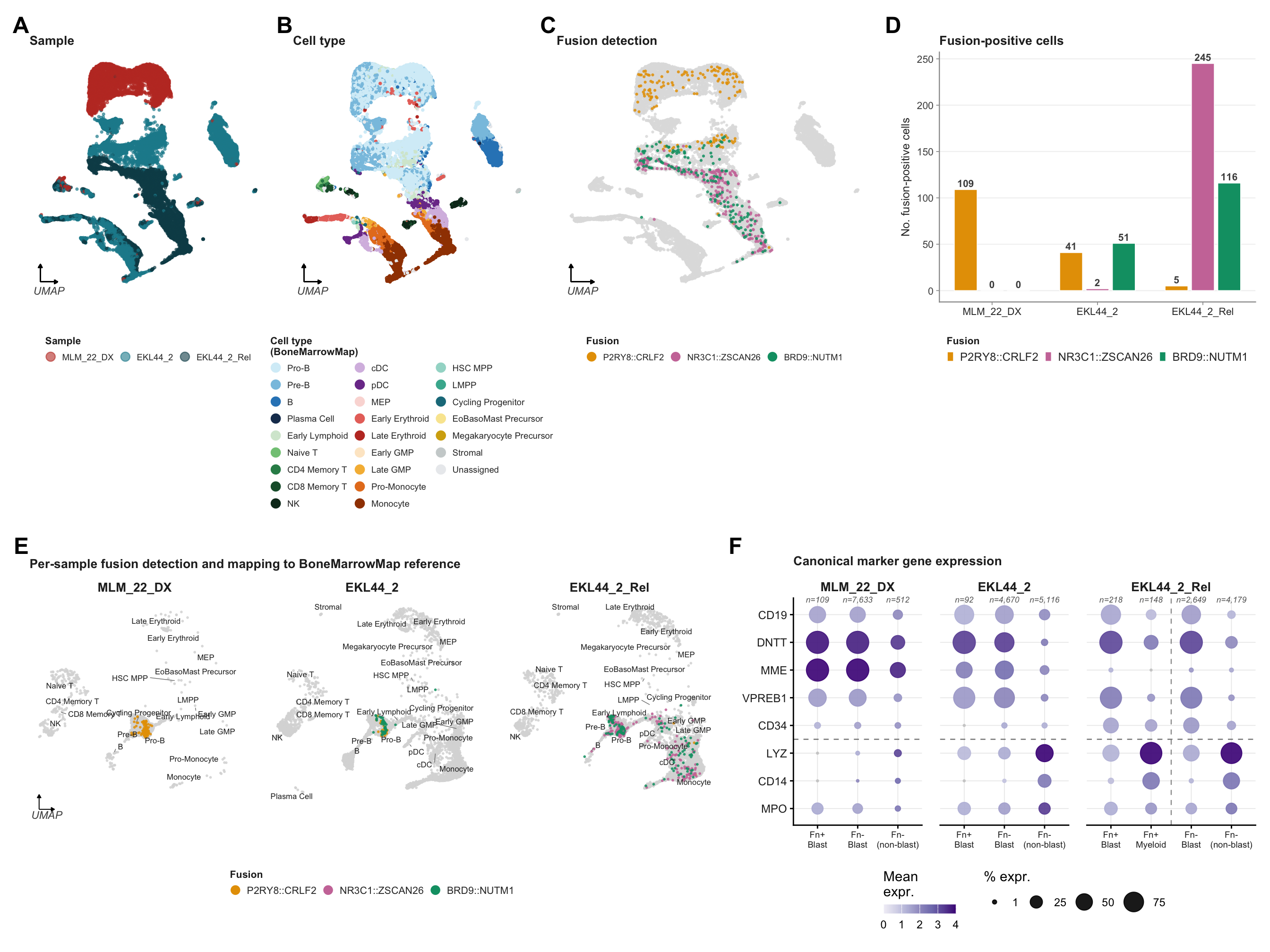
Candidate marker check: LYZ, MPO, VPREB1
Before adding markers to Panel F, check detection rates in the groups
used for that panel. marker_group_f and
marker_facet_f are carried over from the
fig3-full chunk.
candidate_genes <- c("LYZ", "MPO", "VPREB1")

# Confirm which are present in the dataset
present <- candidate_genes[candidate_genes %in% rownames(seu)]
absent  <- setdiff(candidate_genes, present)
if (length(absent)) cat("Not found in dataset:", paste(absent, collapse = ", "), "\n")

cand_counts <- GetAssayData(seu, layer = "counts")[present, , drop = FALSE]
cand_norm   <- GetAssayData(seu, layer = "data")[present,   , drop = FALSE]

base_df <- seu@meta.data %>%
  tibble::rownames_to_column("cell") %>%
  filter(!is.na(marker_group_f), !is.na(marker_facet_f)) %>%
  dplyr::select(cell, marker_group_f, marker_facet_f)

lapply(present, function(gn) {
  counts_vec <- as.numeric(cand_counts[gn, base_df$cell])
  norm_vec   <- as.numeric(cand_norm[gn,   base_df$cell])
  base_df %>%
    mutate(expressed = counts_vec > 0, norm_expr = norm_vec) %>%
    group_by(marker_facet_f, marker_group_f) %>%
    summarise(
      n_cells      = n(),
      pct_det      = round(mean(expressed) * 100, 1),
      mean_expr    = round(ifelse(any(expressed), mean(norm_expr[expressed]), NA_real_), 2),
      .groups      = "drop"
    ) %>%
    mutate(gene = gn)
}) %>%
  bind_rows() %>%
  dplyr::select(gene, marker_facet_f, marker_group_f, n_cells, pct_det, mean_expr) %>%
  arrange(gene, marker_facet_f, marker_group_f) %>%
  knitr::kable(
    col.names = c("Gene", "Sample", "Group", "N cells", "% detected", "Mean expr. (in expressing cells)"),
    caption   = "Detection rates for LYZ, MPO and VPREB1 across Panel F marker groups"
)| Gene | Sample | Group | N cells | % detected | Mean expr. (in expressing cells) |
|---|---|---|---|---|---|
| LYZ | MLM_22_DX | Fn+ | |||
| Blast | 109 | 0.0 | NA | ||
| LYZ | MLM_22_DX | Fn- | |||
| (non-blast) | 512 | 5.9 | 3.18 | ||
| LYZ | MLM_22_DX | Fn- | |||
| Blast | 7633 | 0.8 | 1.33 | ||
| LYZ | EKL44_2 | Fn+ | |||
| Blast | 92 | 28.3 | 1.11 | ||
| LYZ | EKL44_2 | Fn- | |||
| (non-blast) | 5116 | 55.4 | 4.64 | ||
| LYZ | EKL44_2 | Fn- | |||
| Blast | 4670 | 22.2 | 1.40 | ||
| LYZ | EKL44_2_Rel | Fn+ | |||
| Blast | 218 | 48.2 | 1.27 | ||
| LYZ | EKL44_2_Rel | Fn+ | |||
| Myeloid | 148 | 91.9 | 5.13 | ||
| LYZ | EKL44_2_Rel | Fn- | |||
| (non-blast) | 4179 | 85.2 | 5.02 | ||
| LYZ | EKL44_2_Rel | Fn- | |||
| Blast | 2649 | 45.8 | 1.43 | ||
| MPO | MLM_22_DX | Fn+ | |||
| Blast | 109 | 20.2 | 1.41 | ||
| MPO | MLM_22_DX | Fn- | |||
| (non-blast) | 512 | 2.5 | 2.29 | ||
| MPO | MLM_22_DX | Fn- | |||
| Blast | 7633 | 14.2 | 1.53 | ||
| MPO | EKL44_2 | Fn+ | |||
| Blast | 92 | 26.1 | 1.34 | ||
| MPO | EKL44_2 | Fn- | |||
| (non-blast) | 5116 | 20.6 | 3.34 | ||
| MPO | EKL44_2 | Fn- | |||
| Blast | 4670 | 20.7 | 1.59 | ||
| MPO | EKL44_2_Rel | Fn+ | |||
| Blast | 218 | 27.5 | 1.35 | ||
| MPO | EKL44_2_Rel | Fn+ | |||
| Myeloid | 148 | 18.9 | 1.74 | ||
| MPO | EKL44_2_Rel | Fn- | |||
| (non-blast) | 4179 | 18.2 | 2.31 | ||
| MPO | EKL44_2_Rel | Fn- | |||
| Blast | 2649 | 18.0 | 1.46 | ||
| VPREB1 | MLM_22_DX | Fn+ | |||
| Blast | 109 | 57.8 | 1.64 | ||
| VPREB1 | MLM_22_DX | Fn- | |||
| (non-blast) | 512 | 7.4 | 1.77 | ||
| VPREB1 | MLM_22_DX | Fn- | |||
| Blast | 7633 | 53.6 | 1.71 | ||
| VPREB1 | EKL44_2 | Fn+ | |||
| Blast | 92 | 89.1 | 1.71 | ||
| VPREB1 | EKL44_2 | Fn- | |||
| (non-blast) | 5116 | 5.3 | 1.98 | ||
| VPREB1 | EKL44_2 | Fn- | |||
| Blast | 4670 | 78.7 | 2.08 | ||
| VPREB1 | EKL44_2_Rel | Fn+ | |||
| Blast | 218 | 89.4 | 2.23 | ||
| VPREB1 | EKL44_2_Rel | Fn+ | |||
| Myeloid | 148 | 6.1 | 1.75 | ||
| VPREB1 | EKL44_2_Rel | Fn- | |||
| (non-blast) | 4179 | 3.0 | 1.79 | ||
| VPREB1 | EKL44_2_Rel | Fn- | |||
| Blast | 2649 | 86.9 | 2.33 |
Session info
sessioninfo::session_info()─ Session info ───────────────────────────────────────────────────────────────
setting value
version R version 4.4.1 (2024-06-14)
os macOS 15.5
system aarch64, darwin20
ui X11
language (EN)
collate en_US.UTF-8
ctype en_US.UTF-8
tz Australia/Melbourne
date 2026-07-15
pandoc 3.8.3 @ /Applications/RStudio.app/Contents/Resources/app/quarto/bin/tools/aarch64/ (via rmarkdown)
quarto 1.9.38 @ /Applications/RStudio.app/Contents/Resources/app/quarto/bin/quarto
─ Packages ───────────────────────────────────────────────────────────────────
! package * version date (UTC) lib source
P abind 1.4-8 2024-09-12 [?] CRAN (R 4.4.1)
P backports 1.5.0 2024-05-23 [?] CRAN (R 4.4.1)
P Biobase * 2.66.0 2024-11-08 [?] Bioconduc~
P BiocGenerics * 0.52.0 2024-11-08 [?] Bioconduc~
P BiocManager 1.30.27 2025-11-14 [?] CRAN (R 4.4.3)
P bslib 0.9.0 2025-01-30 [?] CRAN (R 4.4.1)
P cachem 1.1.0 2024-05-16 [?] CRAN (R 4.4.1)
P callr 3.7.6 2024-03-25 [?] CRAN (R 4.4.0)
P checkmate 2.3.2 2024-07-29 [?] CRAN (R 4.4.0)
P cli 3.6.5 2025-04-23 [?] CRAN (R 4.4.1)
P cluster 2.1.6 2023-12-01 [?] CRAN (R 4.4.1)
P clustree * 0.5.1 2023-11-05 [?] CRAN (R 4.4.0)
P codetools 0.2-20 2024-03-31 [?] CRAN (R 4.4.1)
P colorspace 2.1-1 2024-07-26 [?] CRAN (R 4.4.1)
P cowplot 1.1.3 2024-01-22 [?] CRAN (R 4.4.0)
P crayon 1.5.3 2024-06-20 [?] CRAN (R 4.4.1)
P data.table 1.18.2.1 2026-01-27 [?] CRAN (R 4.4.3)
P DelayedArray 0.32.0 2024-11-08 [?] Bioconduc~
P deldir 2.0-4 2024-02-28 [?] CRAN (R 4.4.1)
P digest 0.6.37 2024-08-19 [?] CRAN (R 4.4.1)
P dotCall64 1.2 2024-10-04 [?] CRAN (R 4.4.1)
P dplyr * 1.1.4 2023-11-17 [?] CRAN (R 4.4.0)
P evaluate 1.0.3 2025-01-10 [?] CRAN (R 4.4.1)
P farver 2.1.2 2024-05-13 [?] CRAN (R 4.4.1)
P fastDummies 1.7.5 2025-01-20 [?] CRAN (R 4.4.1)
P fastmap 1.2.0 2024-05-15 [?] CRAN (R 4.4.1)
P fitdistrplus 1.2-2 2025-01-07 [?] CRAN (R 4.4.1)
P forcats * 1.0.0 2023-01-29 [?] CRAN (R 4.4.0)
P fs 1.6.6 2025-04-12 [?] CRAN (R 4.4.1)
P future 1.49.0 2025-05-09 [?] CRAN (R 4.4.1)
P future.apply 1.11.3 2024-10-27 [?] CRAN (R 4.4.1)
P generics 0.1.4 2025-05-09 [?] CRAN (R 4.4.1)
P GenomeInfoDb * 1.42.3 2025-01-27 [?] Bioconduc~
P GenomeInfoDbData 1.2.13 2025-05-28 [?] Bioconductor
P GenomicRanges * 1.58.0 2024-11-08 [?] Bioconduc~
P getPass 0.2-4 2023-12-10 [?] CRAN (R 4.4.1)
P ggforce 0.4.2 2024-02-19 [?] CRAN (R 4.4.0)
P ggplot2 * 4.0.2 2026-02-03 [?] CRAN (R 4.4.3)
P ggraph * 2.2.1 2024-03-07 [?] CRAN (R 4.4.0)
P ggrepel * 0.9.6 2024-09-07 [?] CRAN (R 4.4.1)
P ggridges 0.5.6 2024-01-23 [?] CRAN (R 4.4.0)
P git2r 0.36.2 2025-03-29 [?] CRAN (R 4.4.1)
P glmGamPoi * 1.18.0 2024-11-08 [?] Bioconduc~
P globals 0.18.0 2025-05-08 [?] CRAN (R 4.4.1)
P glue * 1.8.0 2024-09-30 [?] CRAN (R 4.4.1)
P goftest 1.2-3 2021-10-07 [?] CRAN (R 4.4.1)
P graphlayouts 1.2.2 2025-01-23 [?] CRAN (R 4.4.1)
P gridExtra 2.3 2017-09-09 [?] CRAN (R 4.4.1)
P gtable 0.3.6 2024-10-25 [?] CRAN (R 4.4.1)
P here * 1.0.1 2020-12-13 [?] CRAN (R 4.4.1)
P hms 1.1.3 2023-03-21 [?] CRAN (R 4.4.0)
P htmltools 0.5.8.1 2024-04-04 [?] CRAN (R 4.4.1)
P htmlwidgets 1.6.4 2023-12-06 [?] CRAN (R 4.4.0)
P httpuv 1.6.16 2025-04-16 [?] CRAN (R 4.4.1)
P httr 1.4.7 2023-08-15 [?] CRAN (R 4.4.0)
P ica 1.0-3 2022-07-08 [?] CRAN (R 4.4.1)
P igraph 2.1.4 2025-01-23 [?] CRAN (R 4.4.1)
P IRanges * 2.40.1 2024-12-05 [?] Bioconduc~
P irlba 2.3.5.1 2022-10-03 [?] CRAN (R 4.4.0)
P jquerylib 0.1.4 2021-04-26 [?] CRAN (R 4.4.0)
P jsonlite 2.0.0 2025-03-27 [?] CRAN (R 4.4.1)
P KernSmooth 2.23-24 2024-05-17 [?] CRAN (R 4.4.1)
P knitr 1.50 2025-03-16 [?] CRAN (R 4.4.1)
P labeling 0.4.3 2023-08-29 [?] CRAN (R 4.4.1)
P later 1.4.2 2025-04-08 [?] CRAN (R 4.4.1)
P lattice 0.22-6 2024-03-20 [?] CRAN (R 4.4.1)
P lazyeval 0.2.2 2019-03-15 [?] CRAN (R 4.4.1)
P lifecycle 1.0.4 2023-11-07 [?] CRAN (R 4.4.1)
P listenv 0.9.1 2024-01-29 [?] CRAN (R 4.4.1)
P lmtest 0.9-40 2022-03-21 [?] CRAN (R 4.4.1)
P lubridate * 1.9.4 2024-12-08 [?] CRAN (R 4.4.1)
P magrittr 2.0.3 2022-03-30 [?] CRAN (R 4.4.1)
P MASS 7.3-60.2 2024-04-26 [?] CRAN (R 4.4.1)
P Matrix 1.7-0 2024-04-26 [?] CRAN (R 4.4.1)
P MatrixGenerics * 1.18.1 2025-01-09 [?] Bioconduc~
P matrixStats * 1.5.0 2025-01-07 [?] CRAN (R 4.4.1)
P memoise 2.0.1 2021-11-26 [?] CRAN (R 4.4.0)
P mime 0.13 2025-03-17 [?] CRAN (R 4.4.1)
P miniUI 0.1.2 2025-04-17 [?] CRAN (R 4.4.1)
P nlme 3.1-164 2023-11-27 [?] CRAN (R 4.4.1)
P paletteer 1.6.0 2024-01-21 [?] CRAN (R 4.4.0)
P parallelly 1.45.0 2025-06-02 [?] CRAN (R 4.4.1)
P patchwork * 1.3.0 2024-09-16 [?] CRAN (R 4.4.1)
P pbapply 1.7-4 2025-07-20 [?] CRAN (R 4.4.1)
P pillar 1.10.2 2025-04-05 [?] CRAN (R 4.4.1)
P pkgconfig 2.0.3 2019-09-22 [?] CRAN (R 4.4.1)
P plotly 4.10.4 2024-01-13 [?] CRAN (R 4.4.0)
P plyr 1.8.9 2023-10-02 [?] CRAN (R 4.4.1)
P png 0.1-8 2022-11-29 [?] CRAN (R 4.4.1)
P polyclip 1.10-7 2024-07-23 [?] CRAN (R 4.4.1)
P prismatic 1.1.2 2024-04-10 [?] CRAN (R 4.4.1)
P processx 3.8.6 2025-02-21 [?] CRAN (R 4.4.1)
P progressr 0.15.1 2024-11-22 [?] CRAN (R 4.4.1)
P promises 1.3.3 2025-05-29 [?] CRAN (R 4.4.1)
P ps 1.9.1 2025-04-12 [?] CRAN (R 4.4.1)
P purrr * 1.0.4 2025-02-05 [?] CRAN (R 4.4.1)
P R6 2.6.1 2025-02-15 [?] CRAN (R 4.4.1)
P RANN 2.6.2 2024-08-25 [?] CRAN (R 4.4.1)
P RColorBrewer 1.1-3 2022-04-03 [?] CRAN (R 4.4.1)
P Rcpp 1.1.1-1.1 2026-04-24 [?] CRAN (R 4.4.1)
P RcppAnnoy 0.0.22 2024-01-23 [?] CRAN (R 4.4.1)
P RcppHNSW 0.6.0 2024-02-04 [?] CRAN (R 4.4.1)
P readr * 2.1.5 2024-01-10 [?] CRAN (R 4.4.0)
P rematch2 2.1.2 2020-05-01 [?] CRAN (R 4.4.0)
renv 1.1.4 2025-03-20 [1] CRAN (R 4.4.1)
P reshape2 1.4.4 2020-04-09 [?] CRAN (R 4.4.0)
P reticulate 1.42.0 2025-03-25 [?] CRAN (R 4.4.1)
P rlang 1.1.6 2025-04-11 [?] CRAN (R 4.4.1)
P rmarkdown 2.29 2024-11-04 [?] CRAN (R 4.4.1)
P ROCR 1.0-11 2020-05-02 [?] CRAN (R 4.4.0)
P rprojroot 2.0.4 2023-11-05 [?] CRAN (R 4.4.1)
P RSpectra 0.16-2 2024-07-18 [?] CRAN (R 4.4.0)
P rstudioapi 0.17.1 2024-10-22 [?] CRAN (R 4.4.1)
P Rtsne 0.17 2023-12-07 [?] CRAN (R 4.4.1)
P S4Arrays 1.6.0 2024-11-08 [?] Bioconduc~
P S4Vectors * 0.44.0 2024-11-08 [?] Bioconduc~
P S7 0.2.0 2024-11-07 [?] CRAN (R 4.4.1)
P sass 0.4.10 2025-04-11 [?] CRAN (R 4.4.1)
P scales * 1.4.0 2025-04-24 [?] CRAN (R 4.4.1)
P scattermore 1.2 2023-06-12 [?] CRAN (R 4.4.0)
P sctransform 0.4.2 2025-04-30 [?] CRAN (R 4.4.1)
P sessioninfo 1.2.3 2025-02-05 [?] CRAN (R 4.4.1)
P Seurat * 5.3.0 2025-04-23 [?] CRAN (R 4.4.1)
P SeuratObject * 5.1.0 2025-04-22 [?] CRAN (R 4.4.1)
P shiny 1.10.0 2024-12-14 [?] CRAN (R 4.4.1)
P SingleCellExperiment * 1.28.1 2024-11-23 [?] Bioconduc~
P sp * 2.2-0 2025-02-01 [?] CRAN (R 4.4.1)
P spam 2.11-1 2025-01-20 [?] CRAN (R 4.4.1)
P SparseArray 1.6.2 2025-02-20 [?] Bioconduc~
P spatstat.data 3.1-6 2025-03-17 [?] CRAN (R 4.4.1)
P spatstat.explore 3.4-3 2025-05-21 [?] CRAN (R 4.4.1)
P spatstat.geom 3.4-1 2025-05-20 [?] CRAN (R 4.4.1)
P spatstat.random 3.4-1 2025-05-20 [?] CRAN (R 4.4.1)
P spatstat.sparse 3.1-0 2024-06-21 [?] CRAN (R 4.4.0)
P spatstat.univar 3.1-3 2025-05-08 [?] CRAN (R 4.4.1)
P spatstat.utils 3.1-4 2025-05-15 [?] CRAN (R 4.4.1)
P stringi 1.8.7 2025-03-27 [?] CRAN (R 4.4.1)
P stringr * 1.6.0 2025-11-04 [?] CRAN (R 4.4.1)
P SummarizedExperiment * 1.36.0 2024-11-08 [?] Bioconduc~
P survival 3.6-4 2024-04-24 [?] CRAN (R 4.4.1)
P tensor 1.5 2012-05-05 [?] CRAN (R 4.4.1)
P tibble * 3.2.1 2023-03-20 [?] CRAN (R 4.4.0)
P tidygraph 1.3.1 2024-01-30 [?] CRAN (R 4.4.0)
P tidyr * 1.3.1 2024-01-24 [?] CRAN (R 4.4.1)
P tidyselect 1.2.1 2024-03-11 [?] CRAN (R 4.4.0)
P tidyverse * 2.0.0 2023-02-22 [?] CRAN (R 4.4.0)
P timechange 0.3.0 2024-01-18 [?] CRAN (R 4.4.1)
P tweenr 2.0.3 2024-02-26 [?] CRAN (R 4.4.0)
P tzdb 0.5.0 2025-03-15 [?] CRAN (R 4.4.1)
P UCSC.utils 1.2.0 2024-11-08 [?] Bioconduc~
P uwot 0.2.3 2025-02-24 [?] CRAN (R 4.4.1)
P vctrs 0.6.5 2023-12-01 [?] CRAN (R 4.4.0)
P viridis 0.6.5 2024-01-29 [?] CRAN (R 4.4.0)
P viridisLite 0.4.2 2023-05-02 [?] CRAN (R 4.4.1)
P whisker 0.4.1 2022-12-05 [?] CRAN (R 4.4.1)
P withr 3.0.2 2024-10-28 [?] CRAN (R 4.4.1)
P workflowr * 1.7.1 2023-08-23 [?] CRAN (R 4.4.0)
P xfun 0.56 2026-01-18 [?] CRAN (R 4.4.3)
P xtable 1.8-4 2019-04-21 [?] CRAN (R 4.4.1)
P XVector 0.46.0 2024-11-08 [?] Bioconduc~
P yaml 2.3.10 2024-07-26 [?] CRAN (R 4.4.1)
P zlibbioc 1.52.0 2024-11-08 [?] Bioconduc~
P zoo 1.8-14 2025-04-10 [?] CRAN (R 4.4.1)
[1] /Users/maksimovicjovana/Library/CloudStorage/OneDrive-PeterMac/Desktop/projects/my_research/flex-fusion-probes/renv/library/macos/R-4.4/aarch64-apple-darwin20
[2] /Users/maksimovicjovana/Library/Caches/org.R-project.R/R/renv/sandbox/macos/R-4.4/aarch64-apple-darwin20/f7156815
* ── Packages attached to the search path.
P ── Loaded and on-disk path mismatch.
──────────────────────────────────────────────────────────────────────────────
sessionInfo()R version 4.4.1 (2024-06-14)
Platform: aarch64-apple-darwin20
Running under: macOS 15.5
Matrix products: default
BLAS: /Library/Frameworks/R.framework/Versions/4.4-arm64/Resources/lib/libRblas.0.dylib
LAPACK: /Library/Frameworks/R.framework/Versions/4.4-arm64/Resources/lib/libRlapack.dylib; LAPACK version 3.12.0
locale:
[1] en_US.UTF-8/en_US.UTF-8/en_US.UTF-8/C/en_US.UTF-8/en_US.UTF-8
time zone: Australia/Melbourne
tzcode source: internal
attached base packages:
[1] stats4 stats graphics grDevices datasets utils methods
[8] base
other attached packages:
[1] ggrepel_0.9.6 glmGamPoi_1.18.0
[3] clustree_0.5.1 ggraph_2.2.1
[5] patchwork_1.3.0 scales_1.4.0
[7] Seurat_5.3.0 SeuratObject_5.1.0
[9] sp_2.2-0 SingleCellExperiment_1.28.1
[11] SummarizedExperiment_1.36.0 Biobase_2.66.0
[13] GenomicRanges_1.58.0 GenomeInfoDb_1.42.3
[15] IRanges_2.40.1 S4Vectors_0.44.0
[17] BiocGenerics_0.52.0 MatrixGenerics_1.18.1
[19] matrixStats_1.5.0 glue_1.8.0
[21] here_1.0.1 lubridate_1.9.4
[23] forcats_1.0.0 stringr_1.6.0
[25] dplyr_1.1.4 purrr_1.0.4
[27] readr_2.1.5 tidyr_1.3.1
[29] tibble_3.2.1 ggplot2_4.0.2
[31] tidyverse_2.0.0 workflowr_1.7.1
loaded via a namespace (and not attached):
[1] RcppAnnoy_0.0.22 splines_4.4.1 later_1.4.2
[4] prismatic_1.1.2 polyclip_1.10-7 fastDummies_1.7.5
[7] lifecycle_1.0.4 rprojroot_2.0.4 globals_0.18.0
[10] processx_3.8.6 lattice_0.22-6 MASS_7.3-60.2
[13] backports_1.5.0 magrittr_2.0.3 plotly_4.10.4
[16] sass_0.4.10 rmarkdown_2.29 jquerylib_0.1.4
[19] yaml_2.3.10 httpuv_1.6.16 sctransform_0.4.2
[22] spam_2.11-1 sessioninfo_1.2.3 spatstat.sparse_3.1-0
[25] reticulate_1.42.0 cowplot_1.1.3 pbapply_1.7-4
[28] RColorBrewer_1.1-3 abind_1.4-8 zlibbioc_1.52.0
[31] Rtsne_0.17 tweenr_2.0.3 git2r_0.36.2
[34] GenomeInfoDbData_1.2.13 irlba_2.3.5.1 listenv_0.9.1
[37] spatstat.utils_3.1-4 goftest_1.2-3 RSpectra_0.16-2
[40] spatstat.random_3.4-1 fitdistrplus_1.2-2 parallelly_1.45.0
[43] codetools_0.2-20 DelayedArray_0.32.0 ggforce_0.4.2
[46] tidyselect_1.2.1 UCSC.utils_1.2.0 farver_2.1.2
[49] viridis_0.6.5 spatstat.explore_3.4-3 jsonlite_2.0.0
[52] tidygraph_1.3.1 progressr_0.15.1 ggridges_0.5.6
[55] survival_3.6-4 tools_4.4.1 ica_1.0-3
[58] Rcpp_1.1.1-1.1 gridExtra_2.3 SparseArray_1.6.2
[61] xfun_0.56 withr_3.0.2 BiocManager_1.30.27
[64] fastmap_1.2.0 callr_3.7.6 digest_0.6.37
[67] timechange_0.3.0 R6_2.6.1 mime_0.13
[70] colorspace_2.1-1 scattermore_1.2 tensor_1.5
[73] spatstat.data_3.1-6 generics_0.1.4 renv_1.1.4
[76] data.table_1.18.2.1 graphlayouts_1.2.2 httr_1.4.7
[79] htmlwidgets_1.6.4 S4Arrays_1.6.0 whisker_0.4.1
[82] uwot_0.2.3 pkgconfig_2.0.3 gtable_0.3.6
[85] lmtest_0.9-40 S7_0.2.0 XVector_0.46.0
[88] htmltools_0.5.8.1 dotCall64_1.2 png_0.1-8
[91] spatstat.univar_3.1-3 knitr_1.50 rstudioapi_0.17.1
[94] tzdb_0.5.0 reshape2_1.4.4 checkmate_2.3.2
[97] nlme_3.1-164 cachem_1.1.0 zoo_1.8-14
[100] KernSmooth_2.23-24 parallel_4.4.1 miniUI_0.1.2
[103] pillar_1.10.2 grid_4.4.1 vctrs_0.6.5
[106] RANN_2.6.2 promises_1.3.3 xtable_1.8-4
[109] cluster_2.1.6 paletteer_1.6.0 evaluate_1.0.3
[112] cli_3.6.5 compiler_4.4.1 rlang_1.1.6
[115] crayon_1.5.3 future.apply_1.11.3 labeling_0.4.3
[118] rematch2_2.1.2 ps_1.9.1 getPass_0.2-4
[121] plyr_1.8.9 fs_1.6.6 stringi_1.8.7
[124] viridisLite_0.4.2 deldir_2.0-4 lazyeval_0.2.2
[127] spatstat.geom_3.4-1 Matrix_1.7-0 RcppHNSW_0.6.0
[130] hms_1.1.3 future_1.49.0 shiny_1.10.0
[133] ROCR_1.0-11 igraph_2.1.4 memoise_2.0.1
[136] bslib_0.9.0