B-ALL Experiment 1: Quality Control

Cell calling, mito% filtering, doublet removal, and MCF7 ambient contamination

workflowr

• Summary
• Checks
• Past versions

Last updated: 2026-07-15

Checks: 7 0

Knit directory: flex-fusion-probes/

This reproducible R Markdown analysis was created with workflowr (version 1.7.1). The Checks tab describes the reproducibility checks that were applied when the results were created. The Past versions tab lists the development history.

---

R Markdown file: up-to-date

Great! Since the R Markdown file has been committed to the Git repository, you know the exact version of the code that produced these results.

Environment: empty

Great job! The global environment was empty. Objects defined in the global environment can affect the analysis in your R Markdown file in unknown ways. For reproduciblity it’s best to always run the code in an empty environment.

Seed: set.seed(20240925)

The command set.seed(20240925) was run prior to running the code in the R Markdown file. Setting a seed ensures that any results that rely on randomness, e.g. subsampling or permutations, are reproducible.

Session information: recorded

Great job! Recording the operating system, R version, and package versions is critical for reproducibility.

Cache: none

Nice! There were no cached chunks for this analysis, so you can be confident that you successfully produced the results during this run.

File paths: relative

Great job! Using relative paths to the files within your workflowr project makes it easier to run your code on other machines.

Repository version: f869e49

Great! You are using Git for version control. Tracking code development and connecting the code version to the results is critical for reproducibility.

The results in this page were generated with repository version f869e49. See the Past versions tab to see a history of the changes made to the R Markdown and HTML files.

Note that you need to be careful to ensure that all relevant files for the analysis have been committed to Git prior to generating the results (you can use wflow_publish or wflow_git_commit). workflowr only checks the R Markdown file, but you know if there are other scripts or data files that it depends on. Below is the status of the Git repository when the results were generated:

Ignored files:
    Ignored:    .DS_Store
    Ignored:    .Rhistory
    Ignored:    .Rproj.user/
    Ignored:    analysis/.gitignore
    Ignored:    analysis/TOM/
    Ignored:    analysis/figure/
    Ignored:    analysis/obsolete/B-ALL_nonblast_fusion_analysis_cache/
    Ignored:    analysis/projectionFigures/
    Ignored:    code/files/
    Ignored:    data/.DS_Store
    Ignored:    data/BoneMarrowMap/
    Ignored:    data/BoneMarrowMapBoneMarrowMap_SymphonyReference.rds
    Ignored:    data/BoneMarrowMapBoneMarrowMap_uwot_model.uwot
    Ignored:    data/CAPTURE-1-POOL-FLEX/
    Ignored:    data/CAPTURE-2-POOL-FLEX/
    Ignored:    data/Pool-240917-FLEX/
    Ignored:    data/RDS/
    Ignored:    data/Run_1_and_Run_2/
    Ignored:    data/Run_2/
    Ignored:    logs/
    Ignored:    output/
    Ignored:    renv/library/
    Ignored:    renv/staging/

Untracked files:
    Untracked:  CLAUDE.md
    Untracked:  analysis/B-ALL_exp2_c1437_clone_analysis.Rmd
    Untracked:  analysis/B-ALL_exp2_c369_mrd_analysis.Rmd
    Untracked:  analysis/B-ALL_exp2_joint_clustering.Rmd
    Untracked:  analysis/fig4_assembly.Rmd
    Untracked:  data/sample_information_flex_experiment_2_table.csv
    Untracked:  poster.pptx

Unstaged changes:
    Modified:   analysis/B-ALL_exp1_annotate_with_BoneMarrowMap.Rmd
    Modified:   analysis/B-ALL_exp1_clustering.Rmd
    Modified:   analysis/B-ALL_exp2_annotate_with_BoneMarrowMap.Rmd
    Deleted:    analysis/B-ALL_exp2_c1437_li2025_clone_analysis.Rmd
    Modified:   analysis/B-ALL_exp2_quality_control.Rmd
    Modified:   analysis/B-ALL_nonblast_fusion_analysis.Rmd
    Modified:   analysis/index.Rmd
    Modified:   render_all.sh

Note that any generated files, e.g. HTML, png, CSS, etc., are not included in this status report because it is ok for generated content to have uncommitted changes.

---

These are the previous versions of the repository in which changes were made to the R Markdown (analysis/B-ALL_exp1_quality_control.Rmd) and HTML (docs/B-ALL_exp1_quality_control.html) files. If you’ve configured a remote Git repository (see ?wflow_git_remote), click on the hyperlinks in the table below to view the files as they were in that past version.

File	Version	Author	Date	Message
Rmd	f869e49	Jovana Maksimovic	2026-07-15	wflow_publish("analysis/B-ALL_exp1_quality_control.Rmd")
html	a8def9a	Jovana Maksimovic	2026-05-18	Build site.
Rmd	08f1e2b	Jovana Maksimovic	2026-05-18	Update index and exp1/exp2 notebooks
html	1b5bb97	Jovana Maksimovic	2026-05-11	Build site.
Rmd	1f3159b	Jovana Maksimovic	2026-05-08	Rename RDS checkpoints to systematic naming scheme
Rmd	1578018	Jovana Maksimovic	2026-05-08	docs: add prose, standardise headings and figure labels across all 10 B-ALL notebooks
Rmd	1a33400	Jovana Maksimovic	2026-05-08	B-ALL cleanup: fix index links, stray library() calls, add chunk labels
Rmd	1724beb	Jovana Maksimovic	2026-05-08	Standardise YAML headers and chunk names across all notebooks; merge utility_functions into utilities.R
Rmd	10d2f5e	Jovana Maksimovic	2026-05-08	Rename analysis notebooks to new naming scheme

---

This notebook performs quality control for B-ALL Experiment 1, which includes three patient samples (MLM_22_DX, EKL44_2_DX, EKL44_2_Rel) and an MCF7 breast cancer cell line control, all multiplexed together in a single Flex capture. Cell calling uses emptyDrops() (FDR < 0.001) combined with the CellRanger knee-point calls (union), which recovers genuine low-UMI cells that the conservative CellRanger algorithm discards. The QC pipeline then covers mito% filtering, doublet detection, and assessment of ambient MCF7 fusion transcript contamination in the B-ALL samples.

The 4-panel contamination figure produced here is Supplementary Figure 3 in the paper.

Load data

emptyDrops() is run on the raw (unfiltered) feature-barcode matrix and the result is cached so that re-running the notebook does not repeat the slow statistical test. Delete exp1_emptydrops.sce.rds to force a fresh run.

ed_rds  <- here("data", "RDS", "exp1_emptydrops.sce.rds")
raw_dir <- here("data", "Run_1_and_Run_2",
                "Cellranger_Config_Sample_Pool-240917-FLEX",
                "outs", "multi", "count", "raw_feature_bc_matrix")
ps_dir  <- here("data", "Run_1_and_Run_2",
                "Cellranger_Config_Sample_Pool-240917-FLEX",
                "outs", "per_sample_outs")

if (file.exists(ed_rds)) {
  cat("Loading cached emptyDrops result ...\n")
  sce <- readRDS(ed_rds)
} else {
  # Collect CellRanger-called barcodes from all per-sample filtered matrices
  filtered_bc <- unlist(lapply(
    list.dirs(ps_dir, full.names = TRUE, recursive = FALSE),
    function(d) {
      bc_file <- file.path(d, "count", "sample_filtered_feature_bc_matrix",
                           "barcodes.tsv.gz")
      if (file.exists(bc_file)) readLines(gzcon(file(bc_file, "rb")))
    }
  ), use.names = FALSE)

  # Load raw (unfiltered) matrix; rename rows to gene symbols
  cat("Loading raw matrix ...\n")
  raw_sce <- read10xCounts(raw_dir, col.names = TRUE)

  # Run emptyDrops; keep union of CellRanger cells and emptyDrops-significant barcodes
  cat("Running emptyDrops (FDR < 0.001) ...\n")
  set.seed(100)
  ed_out  <- emptyDrops(counts(raw_sce))
  ed_sig  <- rownames(ed_out)[!is.na(ed_out$FDR) & ed_out$FDR < 0.001]
  keep_bc <- union(filtered_bc, intersect(colnames(raw_sce), ed_sig))
  sce     <- raw_sce[, colnames(raw_sce) %in% keep_bc]

  # Assign sample labels from probe barcodes (last 8 nt of the cell barcode sequence)
  probe_map <- data.frame(
    probe_bc = c("ACTTTAGG", "AACGGGAA", "AGTAGGCT", "ATGTTGAC"),
    Sample   = c("MCF7", "MLM_22_DX", "EKL44_2_DX", "EKL44_2_Rel"),
    stringsAsFactors = FALSE
  )
  bc_seq     <- sub("-[0-9]+$", "", colnames(sce))
  probe_bcs  <- substr(bc_seq, nchar(bc_seq) - 7L, nchar(bc_seq))
  idx        <- match(probe_bcs, probe_map$probe_bc)
  sce$Sample <- probe_map$Sample[idx]
  sce        <- sce[, !is.na(sce$Sample)]   # drop any unrecognised probe BCs

  cat(glue("Total cells retained: {ncol(sce)}\n"))
  cat("Cells per sample:\n")
  print(table(sce$Sample))

  saveRDS(sce, ed_rds)
  cat(glue("Cached to {ed_rds}\n"))
}

Loading cached emptyDrops result ...

sce <- logNormCounts(sce)
sce

class: SingleCellExperiment 
dim: 37170 39232 
metadata(1): Samples
assays(2): counts logcounts
rownames(37170): ENSG00000243485 ENSG00000237613 ...
  DEPRECATED_ENSG00000284873 DEPRECATED_ENSG00000285687
rowData names(3): ID Symbol Type
colnames(39232): AAACAAGCAACAAGTTACTTTAGG-1 AAACAAGCAACAAGTTAGTAGGCT-1
  ... TTTGTGAGTTGCTCCTAACGGGAA-1 TTTGTGAGTTGCTCCTACTTTAGG-1
colData names(3): Sample Barcode sizeFactor
reducedDimNames(0):
mainExpName: NULL
altExpNames(0):

Data overview

Cells per sample

Overview of cell counts per sample directly from CellRanger output, before any filtering.

p3 <- ggcells(sce) + 
  geom_bar(aes(x = Sample, fill = Sample)) + 
  coord_flip() + 
  ylab("Number of droplets") + 
  geom_text(stat = "count", aes(x = Sample, label = after_stat(count)), 
            hjust=1.5, size=3) +
  guides(fill = "none") +
  theme_bw()

p3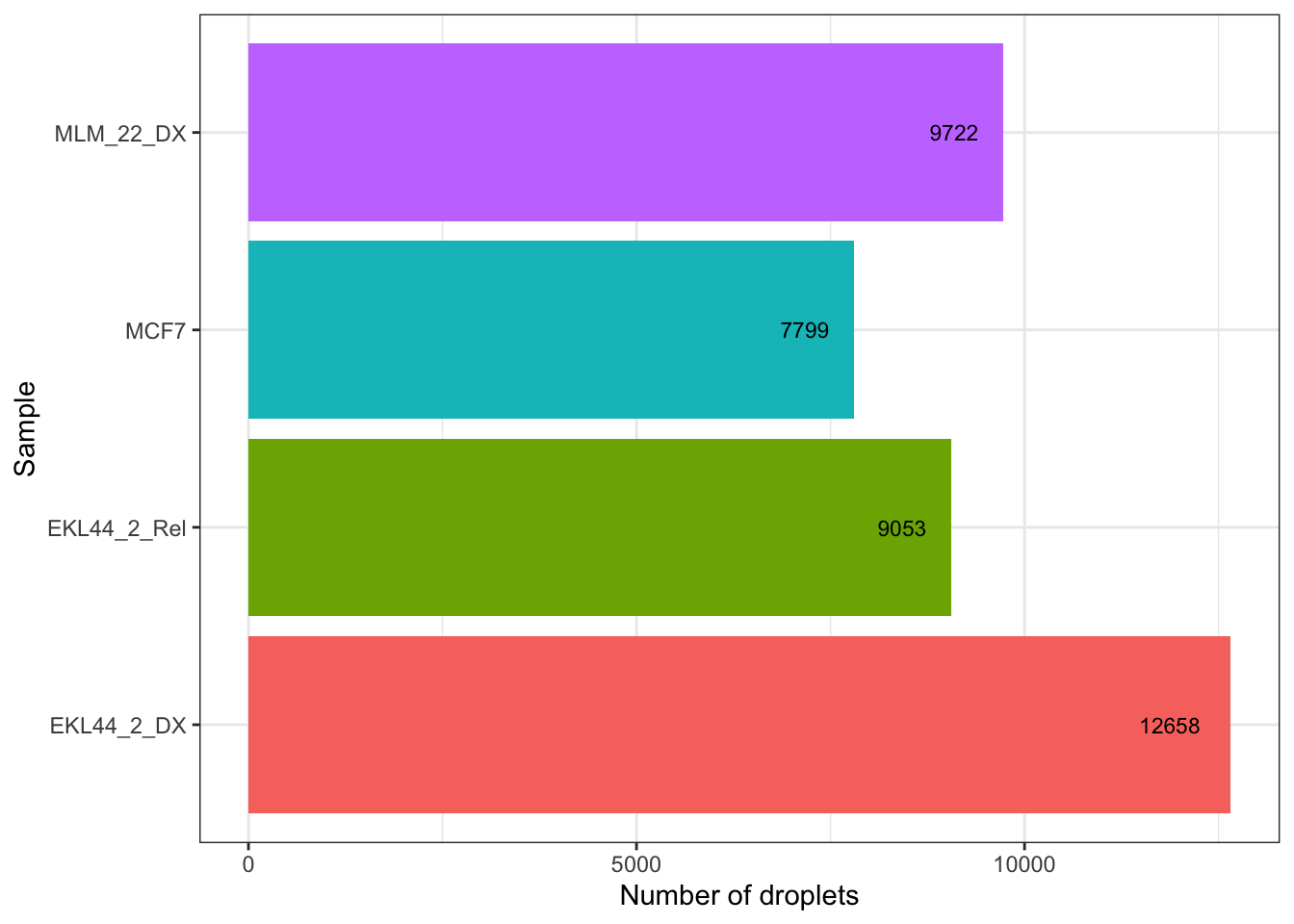 

Past versions of plot-droplets-1.png

Version	Author	Date
1b5bb97	Jovana Maksimovic	2026-05-11

Fusion probe summary

Quick look at the number of fusions assayed and how many UMIs and cells express each fusion, before any QC filtering. Provides a baseline for comparison with post-QC numbers.

sce_fusions <- sce[grepl("fusion", rownames(sce)),]
sce_fusions

class: SingleCellExperiment 
dim: 27 39232 
metadata(1): Samples
assays(2): counts logcounts
rownames(27): FOXA1_TTC6_fusion ARFGEF2_SULF2_fusion ...
  BRD9_NUTM1_fusion NR3C1_ZSCAN26_fusion
rowData names(3): ID Symbol Type
colnames(39232): AAACAAGCAACAAGTTACTTTAGG-1 AAACAAGCAACAAGTTAGTAGGCT-1
  ... TTTGTGAGTTGCTCCTAACGGGAA-1 TTTGTGAGTTGCTCCTACTTTAGG-1
colData names(3): Sample Barcode sizeFactor
reducedDimNames(0):
mainExpName: NULL
altExpNames(0):

The number of fusions assayed is 27.

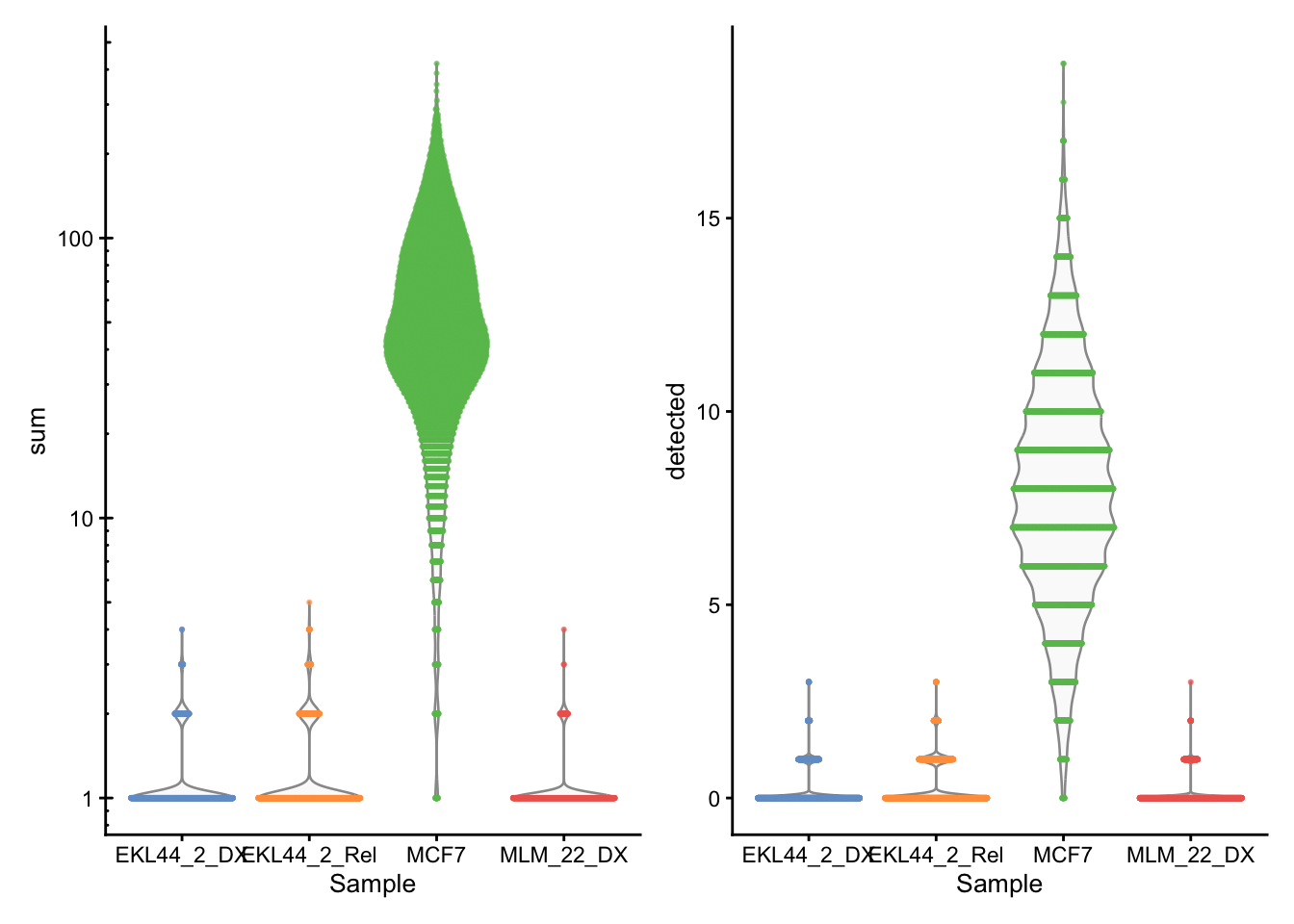
Per cell fusion summary

sce_fusions <- addPerCellQC(sce_fusions)

The library size and number of fusion genes detected per cell in each sample.

p1 <- plotColData(
  sce_fusions,
  "sum",
  x = "Sample",
  colour_by = "Sample",
  point_size = 0.5) +
  scale_y_log10() +
  annotation_logticks(
    sides = "l",
    short = unit(0.03, "cm"),
    mid = unit(0.06, "cm"),
    long = unit(0.09, "cm"))

p2 <- plotColData(
  sce_fusions,
  "detected",
  x = "Sample",
  colour_by = "Sample",
  point_size = 0.5) 

p1 + p2 +
  plot_layout(guides = "collect", ncol = 2) +
  plot_annotation(
    theme = theme(
      legend.position = "none",
      axis.text.x = element_text(angle = 90, hjust = 1, vjust = 0)
    )
  )

Past versions of plot-fusion-qc-1.png

Version	Author	Date
1b5bb97	Jovana Maksimovic	2026-05-11

Total read counts per fusion

fusion_output <- rowSums(counts(sce_fusions)) %>% 
  as.data.frame %>%
  rownames_to_column(var = "Fusion") %>%
  dplyr::rename("Total counts" = ".") %>% knitr::kable()
fusion_output

Fusion	Total counts
FOXA1_TTC6_fusion	4153
ARFGEF2_SULF2_fusion	83291
BCAS4_BCAS3_fusion	103456
YWHAE_MYO1C_fusion	7451
ATXN7_AL355306_2_91741_AL499605_1_328037_fusion	832
ZNF217_SULF2_fusion	33638
ATP9A_RNU7_92P_41182_AL357558_2_5192_fusion	1030
DEPDC1B_ELOVL7_fusion	11894
DDX42_SLC2A10_4301_RN7SKP33_118685_fusion	2967
NCOA3_AL499605_1_36653_AL596327_1_198826_fusion	187669
ATP9A_APCDD1L_fusion	82
RPS6KB1_DIAPH3_fusion	3491
PREX1_LINC01754_44376_RPL35AP_21511_fusion	588
RSBN1_AP4B1_AS1_fusion	1682
EIF2AK3_RPIA_4348_ANKRD36BP2_10530_fusion	1710
TRAPPC4_DSCAML1_fusion	608
TTC6_AL121790_1_fusion	1074
AGFG1_SCYGR1_4229_MIR5703_79954_fusion	299
BCAS3_SNTN_39526_AC104162_1_23281_fusion	1404
SNX14_SNHG5_fusion	136
GCN1_MSI1_fusion	317
USP31_CRYL1_fusion	4241
SGF29_AC244669_2_fusion	1259
ATXN7L3_FAM171A2_fusion	10969
P2RY8_CRLF2_fusion	197
BRD9_NUTM1_fusion	240
NR3C1_ZSCAN26_fusion	327

Read count summary per fusion

sapply(1:nrow(sce_fusions), function(i){
  summary(counts(sce_fusions)[i,])
}) -> fusions_summary

colnames(fusions_summary) <- rownames(sce_fusions)
fusions_summary <- t(fusions_summary)
fusions_summary %>% knitr::kable()

	Min.	1st Qu.	Median	Mean	3rd Qu.	Max.
FOXA1_TTC6_fusion	0	0	0	0.1058575	0	11
ARFGEF2_SULF2_fusion	0	0	0	2.1230373	0	72
BCAS4_BCAS3_fusion	0	0	0	2.6370310	0	106
YWHAE_MYO1C_fusion	0	0	0	0.1899215	0	9
ATXN7_AL355306_2_91741_AL499605_1_328037_fusion	0	0	0	0.0212072	0	3
ZNF217_SULF2_fusion	0	0	0	0.8574123	0	80
ATP9A_RNU7_92P_41182_AL357558_2_5192_fusion	0	0	0	0.0262541	0	3
DEPDC1B_ELOVL7_fusion	0	0	0	0.3031709	0	20
DDX42_SLC2A10_4301_RN7SKP33_118685_fusion	0	0	0	0.0756270	0	6
NCOA3_AL499605_1_36653_AL596327_1_198826_fusion	0	0	0	4.7835695	1	176
ATP9A_APCDD1L_fusion	0	0	0	0.0020901	0	2
RPS6KB1_DIAPH3_fusion	0	0	0	0.0889835	0	7
PREX1_LINC01754_44376_RPL35AP_21511_fusion	0	0	0	0.0149878	0	5
RSBN1_AP4B1_AS1_fusion	0	0	0	0.0428732	0	7
EIF2AK3_RPIA_4348_ANKRD36BP2_10530_fusion	0	0	0	0.0435869	0	4
TRAPPC4_DSCAML1_fusion	0	0	0	0.0154976	0	2
TTC6_AL121790_1_fusion	0	0	0	0.0273756	0	5
AGFG1_SCYGR1_4229_MIR5703_79954_fusion	0	0	0	0.0076213	0	3
BCAS3_SNTN_39526_AC104162_1_23281_fusion	0	0	0	0.0357871	0	4
SNX14_SNHG5_fusion	0	0	0	0.0034666	0	2
GCN1_MSI1_fusion	0	0	0	0.0080801	0	3
USP31_CRYL1_fusion	0	0	0	0.1081005	0	9
SGF29_AC244669_2_fusion	0	0	0	0.0320912	0	3
ATXN7L3_FAM171A2_fusion	0	0	0	0.2795932	0	12
P2RY8_CRLF2_fusion	0	0	0	0.0050214	0	2
BRD9_NUTM1_fusion	0	0	0	0.0061175	0	2
NR3C1_ZSCAN26_fusion	0	0	0	0.0083350	0	2

No. cells expressing each fusion per sample

lapply(levels(factor(sce$Sample)), function(samp){
nexprs(sce_fusions[, sce_fusions$Sample == samp], byrow = TRUE) %>%
  as.data.frame() %>%
  rownames_to_column(var = "Fusion") %>%
  dplyr::rename("No. cells with counts > 0" = ".") %>% 
    knitr::kable(caption = samp)
})

[[1]]


Table: EKL44_2_DX

|Fusion                                          | No. cells with counts > 0|
|:-----------------------------------------------|-------------------------:|
|FOXA1_TTC6_fusion                               |                         0|
|ARFGEF2_SULF2_fusion                            |                       149|
|BCAS4_BCAS3_fusion                              |                         7|
|YWHAE_MYO1C_fusion                              |                       210|
|ATXN7_AL355306_2_91741_AL499605_1_328037_fusion |                         0|
|ZNF217_SULF2_fusion                             |                        16|
|ATP9A_RNU7_92P_41182_AL357558_2_5192_fusion     |                        13|
|DEPDC1B_ELOVL7_fusion                           |                        17|
|DDX42_SLC2A10_4301_RN7SKP33_118685_fusion       |                         0|
|NCOA3_AL499605_1_36653_AL596327_1_198826_fusion |                      1142|
|ATP9A_APCDD1L_fusion                            |                         0|
|RPS6KB1_DIAPH3_fusion                           |                         0|
|PREX1_LINC01754_44376_RPL35AP_21511_fusion      |                         0|
|RSBN1_AP4B1_AS1_fusion                          |                         0|
|EIF2AK3_RPIA_4348_ANKRD36BP2_10530_fusion       |                         0|
|TRAPPC4_DSCAML1_fusion                          |                         0|
|TTC6_AL121790_1_fusion                          |                         0|
|AGFG1_SCYGR1_4229_MIR5703_79954_fusion          |                         0|
|BCAS3_SNTN_39526_AC104162_1_23281_fusion        |                         0|
|SNX14_SNHG5_fusion                              |                         0|
|GCN1_MSI1_fusion                                |                         0|
|USP31_CRYL1_fusion                              |                        42|
|SGF29_AC244669_2_fusion                         |                        20|
|ATXN7L3_FAM171A2_fusion                         |                       766|
|P2RY8_CRLF2_fusion                              |                        54|
|BRD9_NUTM1_fusion                               |                        89|
|NR3C1_ZSCAN26_fusion                            |                         6|

[[2]]


Table: EKL44_2_Rel

|Fusion                                          | No. cells with counts > 0|
|:-----------------------------------------------|-------------------------:|
|FOXA1_TTC6_fusion                               |                         1|
|ARFGEF2_SULF2_fusion                            |                        44|
|BCAS4_BCAS3_fusion                              |                         5|
|YWHAE_MYO1C_fusion                              |                         4|
|ATXN7_AL355306_2_91741_AL499605_1_328037_fusion |                         0|
|ZNF217_SULF2_fusion                             |                       123|
|ATP9A_RNU7_92P_41182_AL357558_2_5192_fusion     |                        14|
|DEPDC1B_ELOVL7_fusion                           |                         4|
|DDX42_SLC2A10_4301_RN7SKP33_118685_fusion       |                         0|
|NCOA3_AL499605_1_36653_AL596327_1_198826_fusion |                      1463|
|ATP9A_APCDD1L_fusion                            |                         0|
|RPS6KB1_DIAPH3_fusion                           |                         0|
|PREX1_LINC01754_44376_RPL35AP_21511_fusion      |                         0|
|RSBN1_AP4B1_AS1_fusion                          |                         0|
|EIF2AK3_RPIA_4348_ANKRD36BP2_10530_fusion       |                         0|
|TRAPPC4_DSCAML1_fusion                          |                         0|
|TTC6_AL121790_1_fusion                          |                         0|
|AGFG1_SCYGR1_4229_MIR5703_79954_fusion          |                         0|
|BCAS3_SNTN_39526_AC104162_1_23281_fusion        |                         0|
|SNX14_SNHG5_fusion                              |                         0|
|GCN1_MSI1_fusion                                |                         0|
|USP31_CRYL1_fusion                              |                        45|
|SGF29_AC244669_2_fusion                         |                        14|
|ATXN7L3_FAM171A2_fusion                         |                       682|
|P2RY8_CRLF2_fusion                              |                         6|
|BRD9_NUTM1_fusion                               |                       147|
|NR3C1_ZSCAN26_fusion                            |                       308|

[[3]]


Table: MCF7

|Fusion                                          | No. cells with counts > 0|
|:-----------------------------------------------|-------------------------:|
|FOXA1_TTC6_fusion                               |                      2870|
|ARFGEF2_SULF2_fusion                            |                      7533|
|BCAS4_BCAS3_fusion                              |                      7396|
|YWHAE_MYO1C_fusion                              |                      4106|
|ATXN7_AL355306_2_91741_AL499605_1_328037_fusion |                       754|
|ZNF217_SULF2_fusion                             |                      6863|
|ATP9A_RNU7_92P_41182_AL357558_2_5192_fusion     |                       909|
|DEPDC1B_ELOVL7_fusion                           |                      4327|
|DDX42_SLC2A10_4301_RN7SKP33_118685_fusion       |                      2272|
|NCOA3_AL499605_1_36653_AL596327_1_198826_fusion |                      7727|
|ATP9A_APCDD1L_fusion                            |                        80|
|RPS6KB1_DIAPH3_fusion                           |                      2491|
|PREX1_LINC01754_44376_RPL35AP_21511_fusion      |                       542|
|RSBN1_AP4B1_AS1_fusion                          |                      1409|
|EIF2AK3_RPIA_4348_ANKRD36BP2_10530_fusion       |                      1448|
|TRAPPC4_DSCAML1_fusion                          |                       582|
|TTC6_AL121790_1_fusion                          |                       927|
|AGFG1_SCYGR1_4229_MIR5703_79954_fusion          |                       286|
|BCAS3_SNTN_39526_AC104162_1_23281_fusion        |                      1204|
|SNX14_SNHG5_fusion                              |                       134|
|GCN1_MSI1_fusion                                |                       302|
|USP31_CRYL1_fusion                              |                      2906|
|SGF29_AC244669_2_fusion                         |                      1087|
|ATXN7L3_FAM171A2_fusion                         |                      4572|
|P2RY8_CRLF2_fusion                              |                         0|
|BRD9_NUTM1_fusion                               |                         0|
|NR3C1_ZSCAN26_fusion                            |                         0|

[[4]]


Table: MLM_22_DX

|Fusion                                          | No. cells with counts > 0|
|:-----------------------------------------------|-------------------------:|
|FOXA1_TTC6_fusion                               |                         0|
|ARFGEF2_SULF2_fusion                            |                         4|
|BCAS4_BCAS3_fusion                              |                         1|
|YWHAE_MYO1C_fusion                              |                         6|
|ATXN7_AL355306_2_91741_AL499605_1_328037_fusion |                         0|
|ZNF217_SULF2_fusion                             |                         1|
|ATP9A_RNU7_92P_41182_AL357558_2_5192_fusion     |                         5|
|DEPDC1B_ELOVL7_fusion                           |                         2|
|DDX42_SLC2A10_4301_RN7SKP33_118685_fusion       |                         0|
|NCOA3_AL499605_1_36653_AL596327_1_198826_fusion |                       853|
|ATP9A_APCDD1L_fusion                            |                         0|
|RPS6KB1_DIAPH3_fusion                           |                         0|
|PREX1_LINC01754_44376_RPL35AP_21511_fusion      |                         0|
|RSBN1_AP4B1_AS1_fusion                          |                         0|
|EIF2AK3_RPIA_4348_ANKRD36BP2_10530_fusion       |                         0|
|TRAPPC4_DSCAML1_fusion                          |                         0|
|TTC6_AL121790_1_fusion                          |                         0|
|AGFG1_SCYGR1_4229_MIR5703_79954_fusion          |                         0|
|BCAS3_SNTN_39526_AC104162_1_23281_fusion        |                         0|
|SNX14_SNHG5_fusion                              |                         0|
|GCN1_MSI1_fusion                                |                         0|
|USP31_CRYL1_fusion                              |                         5|
|SGF29_AC244669_2_fusion                         |                         0|
|ATXN7L3_FAM171A2_fusion                         |                       206|
|P2RY8_CRLF2_fusion                              |                       134|
|BRD9_NUTM1_fusion                               |                         0|
|NR3C1_ZSCAN26_fusion                            |                         0|

Fusion expression per sample

fusions <- str_detect(rownames(sce), "fusion")
plotExpression(sce, 
               rownames(sce)[fusions],
               x = "Sample",
               colour_by = "Sample",
               point_size = 1) -> p1

p1 + theme(legend.position = "none")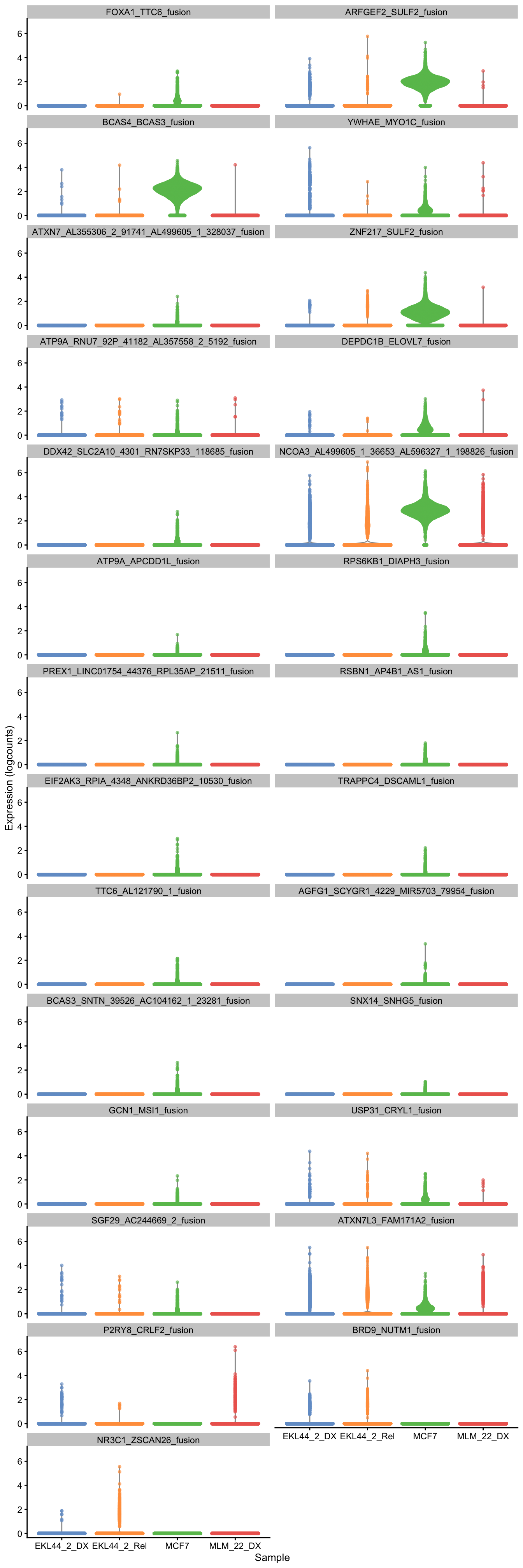

Past versions of plot-fusion-expression-1.png

Version	Author	Date
1b5bb97	Jovana Maksimovic	2026-05-11

Patient fusion per cell

Label fusion-expressing cells.

patient_fusions <- c("P2RY8_CRLF2_fusion", "BRD9_NUTM1_fusion", "NR3C1_ZSCAN26_fusion")
patient_fusions_detected <- colSums(counts(sce)[rownames(sce) %in% patient_fusions,]) > 0

table(patient_fusions_detected)

patient_fusions_detected
FALSE  TRUE 
38496   736 

fusion_type <- ifelse(counts(sce)[rownames(sce) == patient_fusions[1], ] > 0,
                      patient_fusions[1], 
                      ifelse(counts(sce)[rownames(sce) == patient_fusions[2], ] > 0,
                      patient_fusions[2],
                      ifelse(counts(sce)[rownames(sce) == patient_fusions[3], ] > 0,
                      patient_fusions[3], "not-detected")))

sce$patient_fusion <- fusion_type

table(sce$patient_fusion, sce$Sample)

                      
                       EKL44_2_DX EKL44_2_Rel  MCF7 MLM_22_DX
  BRD9_NUTM1_fusion            88         147     0         0
  not-detected              12510        8599  7799      9588
  NR3C1_ZSCAN26_fusion          6         301     0         0
  P2RY8_CRLF2_fusion           54           6     0       134

table(colSums(counts(sce)[rownames(sce) %in% patient_fusions, sce$patient_fusion != "not-detected"]))

  1   2   3 
709  26   1 

sce$patient_fusion_detected <- sce$patient_fusion != "not-detected"

colData(sce) %>%
  data.frame %>%
  rownames_to_column(var = "cell_id") %>%
  group_by(cell_id) %>%
  mutate(n = sum(patient_fusion_detected)) %>%
  filter(n > 1) 

# A tibble: 0 × 7
# Groups:   cell_id [0]
# ℹ 7 variables: cell_id <chr>, Sample <chr>, Barcode <chr>, sizeFactor <dbl>,
#   patient_fusion <chr>, patient_fusion_detected <lgl>, n <int>

Quality control

Cells are filtered based on mitochondrial read percentage. Outliers are defined per sample using the median absolute deviation (MAD) method (3 MADs above the median), which accounts for sample-specific differences in sequencing depth and cell biology.

Identify mitochondrial genes.

rowData(sce)$is_mito <- str_detect(rowData(sce)$Symbol, "^MT-")

Calculate per cell quality control metrics.

sce <- addPerCellQC(sce,
                    subsets = list(is_mito = rowData(sce)$is_mito))

Per cell QC

p1 <- plotColData(
  sce,
  "sum",
  x = "Sample",
  colour_by = "Sample",
  point_size = 0.5) +
  scale_y_log10() +
  annotation_logticks(
    sides = "l",
    short = unit(0.03, "cm"),
    mid = unit(0.06, "cm"),
    long = unit(0.09, "cm"))

p2 <- plotColData(
  sce,
  "detected",
  x = "Sample",
  colour_by = "Sample",
  point_size = 0.5) 

p3 <- plotColData(
  sce,
  "subsets_is_mito_percent",
  x = "Sample",
  colour_by = "Sample",
  point_size = 0.5) 

axis_theme <- theme(
  axis.text.x = element_text(angle = 90, hjust = 1, vjust = 0)
)

p1 <- p1 + axis_theme
p2 <- p2 + axis_theme
p3 <- p3 + axis_theme

p1 + p2 + p3 +
  plot_layout(guides = "collect", ncol = 2) +
  plot_annotation(theme = theme(legend.position = "none"))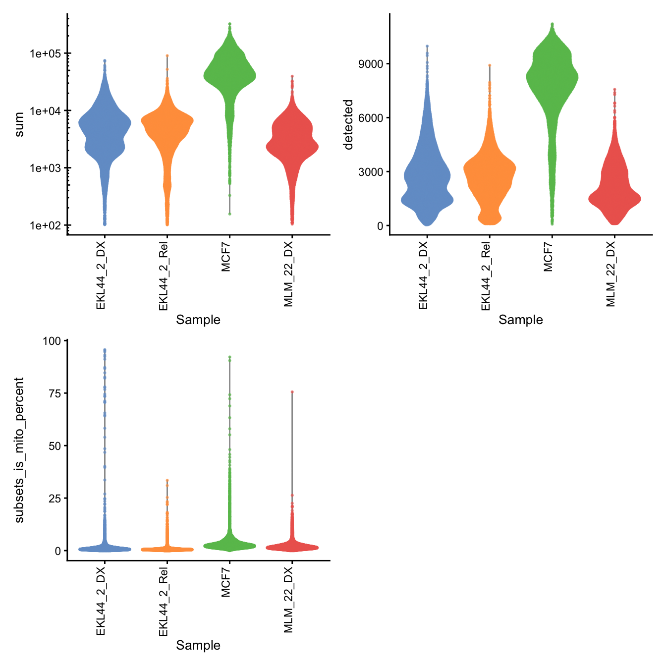

Past versions of plot-qc-metrics-1.png

Version	Author	Date
1b5bb97	Jovana Maksimovic	2026-05-11

Identify outliers by mitochondrial read %

Filtering on the mitochondrial proportion can identify stressed/damaged cells and so we seek to identify droplets with unusually large mitochondrial proportions (i.e. outliers). Outlier thresholds are defined based on the median absolute deviation (MADs) from the median value of the metric across all cells. Here, we opt to use sample-specific thresholds to account for sample-specific differences.

sce$Sample <- factor(sce$Sample)

mito_drop <- isOutlier(
  metric = sce$subsets_is_mito_percent,
  nmads = 3,
  type = "higher",
  batch = sce$Sample)
mito_drop_df <- data.frame(
  sample = factor(
    colnames(attributes(mito_drop)$thresholds),
    levels(sce$Sample)),
  lower = attributes(mito_drop)$thresholds["higher", ])

The following table summarises the QC cutoffs:

mito_drop_df %>%
  knitr::kable()

	sample	lower
EKL44_2_DX	EKL44_2_DX	2.918572
EKL44_2_Rel	EKL44_2_Rel	1.574824
MCF7	MCF7	7.349077
MLM_22_DX	MLM_22_DX	4.963800

The majority of cells are retained for all samples.

data.frame(drop = mito_drop,
           Sample = sce$Sample) %>%
  group_by(Sample) %>%
  summarise(Drop = sum(drop),
            Keep = n() - sum(drop),
            PctKeep = (n() - sum(drop))/n()*100) %>%
  knitr::kable()

Sample	Drop	Keep	PctKeep
EKL44_2_DX	906	11752	92.84247
EKL44_2_Rel	708	8345	92.17939
MCF7	554	7245	92.89653
MLM_22_DX	548	9174	94.36330

Tag cell that will be dropped.

sce$mito_keep <- !mito_drop

Identify outliers by genes detected (lower bound)

Cells with very few genes detected relative to their peers may represent empty droplets that passed emptyDrops or highly degraded cells. A lower-bound outlier threshold is defined per sample using 3 MADs below the median on the log scale.

gene_drop <- isOutlier(
  metric = sce$detected,
  nmads  = 3,
  type   = "lower",
  log    = TRUE,
  batch  = sce$Sample)

gene_drop_df <- data.frame(
  sample    = colnames(attributes(gene_drop)$thresholds),
  threshold = attributes(gene_drop)$thresholds["lower", ],
  row.names = NULL)

gene_drop_df %>% knitr::kable(row.names = FALSE)

sample	threshold
EKL44_2_DX	395.6369
EKL44_2_Rel	756.9724
MCF7	4720.5150
MLM_22_DX	305.7197

data.frame(drop = gene_drop, sample = sce$Sample) %>%
  group_by(sample) %>%
  summarise(Drop    = sum(drop),
            Keep    = n() - sum(drop),
            PctKeep = round((n() - sum(drop)) / n() * 100, 1)) %>%
  knitr::kable(row.names = FALSE)

sample	Drop	Keep	PctKeep
EKL44_2_DX	281	12377	97.8
EKL44_2_Rel	832	8221	90.8
MCF7	726	7073	90.7
MLM_22_DX	188	9534	98.1

sce$gene_keep <- !gene_drop

Combined filter summary

sce$keep_all <- sce$mito_keep & sce$gene_keep

colData(sce) %>%
  data.frame() %>%
  group_by(Sample) %>%
  summarise(
    N_total    = n(),
    Drop_mito  = sum(!mito_keep),
    Drop_genes = sum(!gene_keep),
    Drop_any   = sum(!keep_all),
    PctKeep    = round(sum(keep_all) / n() * 100, 1)
  ) %>%
  knitr::kable(caption = "Cells removed by each filter and combined",
               row.names = FALSE)

Cells removed by each filter and combined

Sample	N_total	Drop_mito	Drop_genes	Drop_any	PctKeep
EKL44_2_DX	12658	906	281	1110	91.2
EKL44_2_Rel	9053	708	832	1213	86.6
MCF7	7799	554	726	968	87.6
MLM_22_DX	9722	548	188	683	93.0

Scatter plot of total UMI vs. genes detected coloured by filter outcome, to visually confirm thresholds are sensible.

colData(sce) %>%
  data.frame() %>%
  mutate(
    filter_result = case_when(
      !mito_keep ~ "High mito",
      !gene_keep ~ "Low genes",
      TRUE       ~ "Keep"
    ),
    filter_result = factor(filter_result,
                           levels = c("Keep", "High mito", "Low genes"))
  ) %>%
  ggplot(aes(x = sum, y = detected,
             colour = filter_result, alpha = filter_result)) +
  geom_point(size = 0.3) +
  scale_x_log10(labels = scales::comma) +
  scale_y_log10(labels = scales::comma) +
  scale_colour_manual(values = c("Keep"      = "grey70",
                                 "High mito" = "#E41A1C",
                                 "Low genes" = "#377EB8")) +
  scale_alpha_manual(values  = c("Keep"      = 0.2,
                                 "High mito" = 0.8,
                                 "Low genes" = 0.8)) +
  facet_wrap(~ Sample, ncol = 2) +
  labs(x = "Total UMI (log scale)", y = "Genes detected (log scale)",
       colour = "Filter", alpha = "Filter") +
  theme_classic(base_size = 9) +
  guides(colour = guide_legend(override.aes = list(size = 2, alpha = 1)))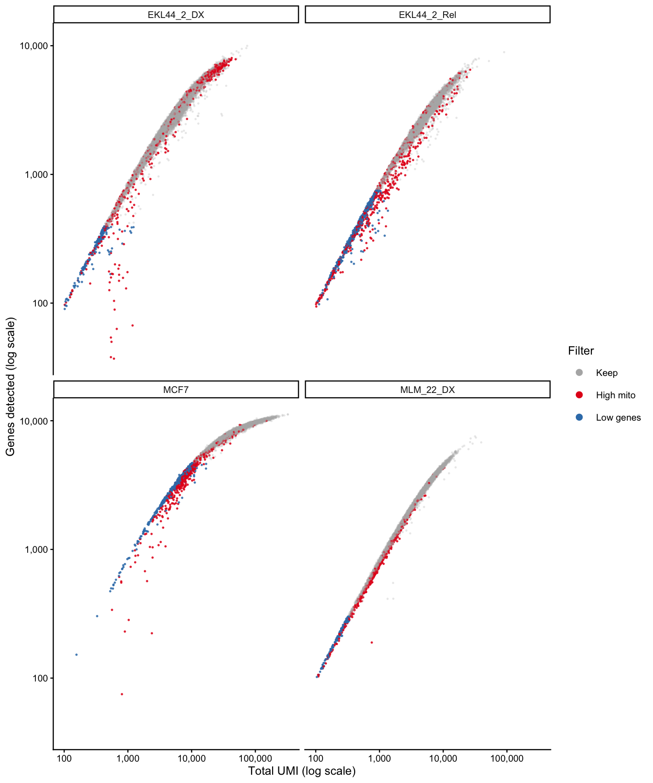

Cells to discard per sample

Another concern is whether the cells removed during QC preferentially derive from particular experimental groups. Reassuringly, the following figure shows that this is not the case.

ggcells(sce) +
  geom_bar(aes(x = Sample, fill = mito_keep)) +
  ylab("Number of droplets") +
  theme(axis.text.x = element_text(angle = 45, hjust = 1)) +
  facet_grid(Sample ~ ., scales = "free_y") +
  theme_bw()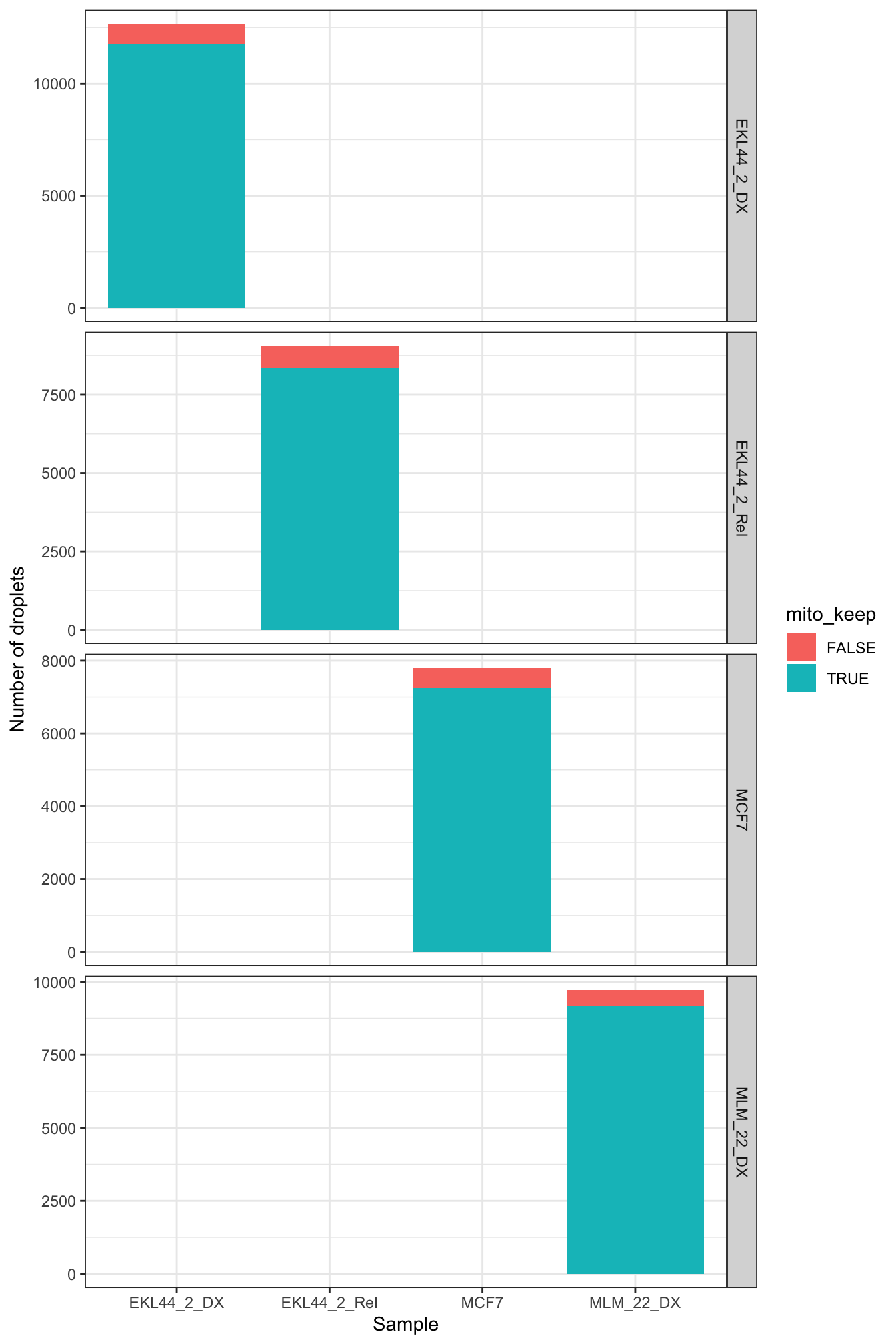

Past versions of plot-discard-1.png

Version	Author	Date
1b5bb97	Jovana Maksimovic	2026-05-11

QC metrics of poor vs. good quality cells

Finally, this figure compares the QC metrics of the discarded and retained droplets.

p1 <- plotColData(
  sce,
  "sum",
  x = "Sample",
  colour_by = "mito_keep",
  point_size = 0.5) +
  scale_y_log10() +
  theme(axis.text.x = element_text(angle = 45, hjust = 1)) +
  annotation_logticks(
    sides = "l",
    short = unit(0.03, "cm"),
    mid = unit(0.06, "cm"),
    long = unit(0.09, "cm"))
p2 <- plotColData(
  sce,
  "detected",
  x = "Sample",
  colour_by = "mito_keep",
  point_size = 0.5) +
  theme(axis.text.x = element_text(angle = 45, hjust = 1))
p3 <- plotColData(
  sce,
  "subsets_is_mito_percent",
  x = "Sample",
  colour_by = "mito_keep",
  point_size = 0.5) +
  theme(axis.text.x = element_text(angle = 45, hjust = 1))

p1 + p2 + p3 + plot_layout(guides = "collect")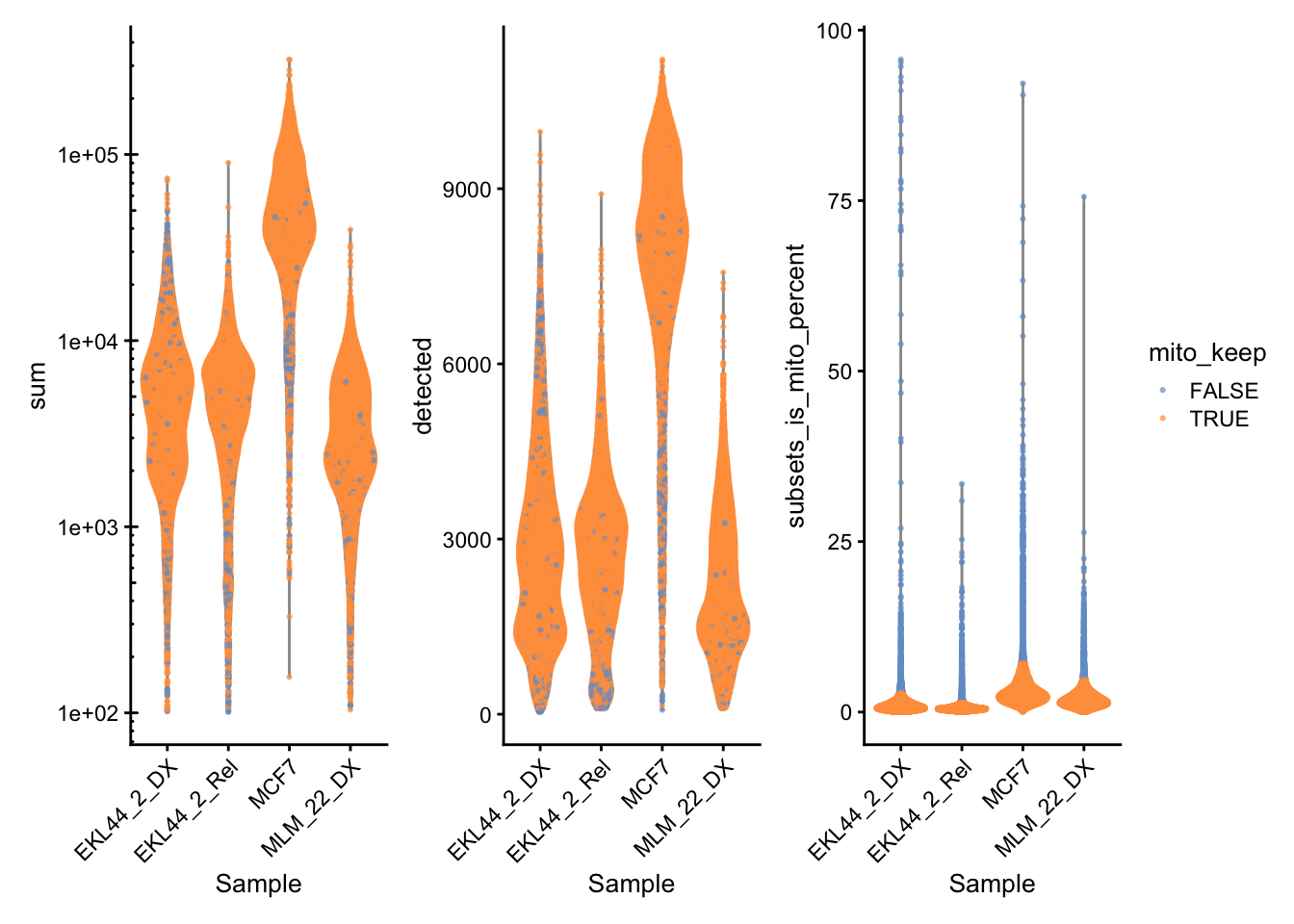

Past versions of plot-qc-good-vs-bad-1.png

Version	Author	Date
1b5bb97	Jovana Maksimovic	2026-05-11

Apply combined filter (mito % + genes detected).

sub <- sce[, sce$keep_all]
sub

class: SingleCellExperiment 
dim: 37170 35258 
metadata(1): Samples
assays(2): counts logcounts
rownames(37170): ENSG00000243485 ENSG00000237613 ...
  DEPRECATED_ENSG00000284873 DEPRECATED_ENSG00000285687
rowData names(5): ID Symbol Type is_mito subsets_is_mito
colnames(35258): AAACAAGCAACAAGTTACTTTAGG-1 AAACAAGCAACAAGTTAGTAGGCT-1
  ... TTTGTGAGTTGCTCCTAACGGGAA-1 TTTGTGAGTTGCTCCTACTTTAGG-1
colData names(14): Sample Barcode ... gene_keep keep_all
reducedDimNames(0):
mainExpName: NULL
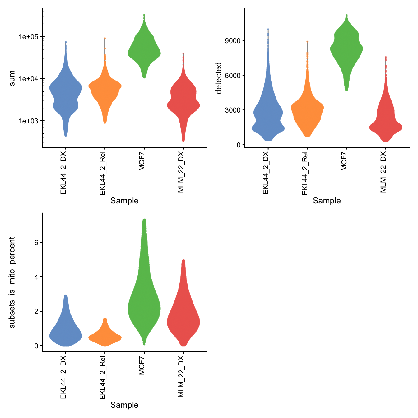
altExpNames(0):

Per cell QC after mito % filtering

p1 <- plotColData(
  sub,
  "sum",
  x = "Sample",
  colour_by = "Sample",
  point_size = 0.5) +
  scale_y_log10() +
  annotation_logticks(
    sides = "l",
    short = unit(0.03, "cm"),
    mid = unit(0.06, "cm"),
    long = unit(0.09, "cm"))
p2 <- plotColData(
  sub,
  "detected",
  x = "Sample",
  colour_by = "Sample",
  point_size = 0.5)
p3 <- plotColData(
  sub,
  "subsets_is_mito_percent",
  x = "Sample",
  colour_by = "Sample",
  point_size = 0.5)

# Define the axis text rotation theme
axis_theme <- theme(
  axis.text.x = element_text(angle = 90, hjust = 1, vjust = 0)
)

# Apply to each plot individually
p1 <- p1 + axis_theme
p2 <- p2 + axis_theme
p3 <- p3 + axis_theme

# Combine plots with patchwork
p1 + p2 + p3 +
  plot_layout(guides = "collect", ncol = 2) +
  plot_annotation(
    theme = theme(
      legend.position = "none"
    )
  )

Past versions of plot-qc-post-filter-1.png

Version	Author	Date
1b5bb97	Jovana Maksimovic	2026-05-11

No. non-empty droplets after mito % filtering

p3 <- ggcells(sub) +
  geom_bar(aes(x = Sample, fill = Sample)) +
  coord_flip() +
  ylab("Number of droplets") +
  geom_text(stat='count', aes(x = Sample, label = after_stat(count)), hjust=1.5, size=3) +
  guides(fill = "none") +
  theme_bw()

p3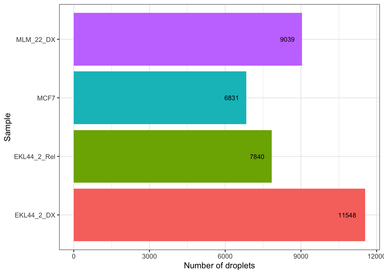

Past versions of plot-droplets-post-filter-1.png

Version	Author	Date
1b5bb97	Jovana Maksimovic	2026-05-11

Fusion expression after mito % filtering

plotExpression(sub, 
               rownames(sub)[fusions],
               x = "Sample",
               colour_by = "Sample",
               point_size = 1) -> p1

p1 + theme(legend.position = "none")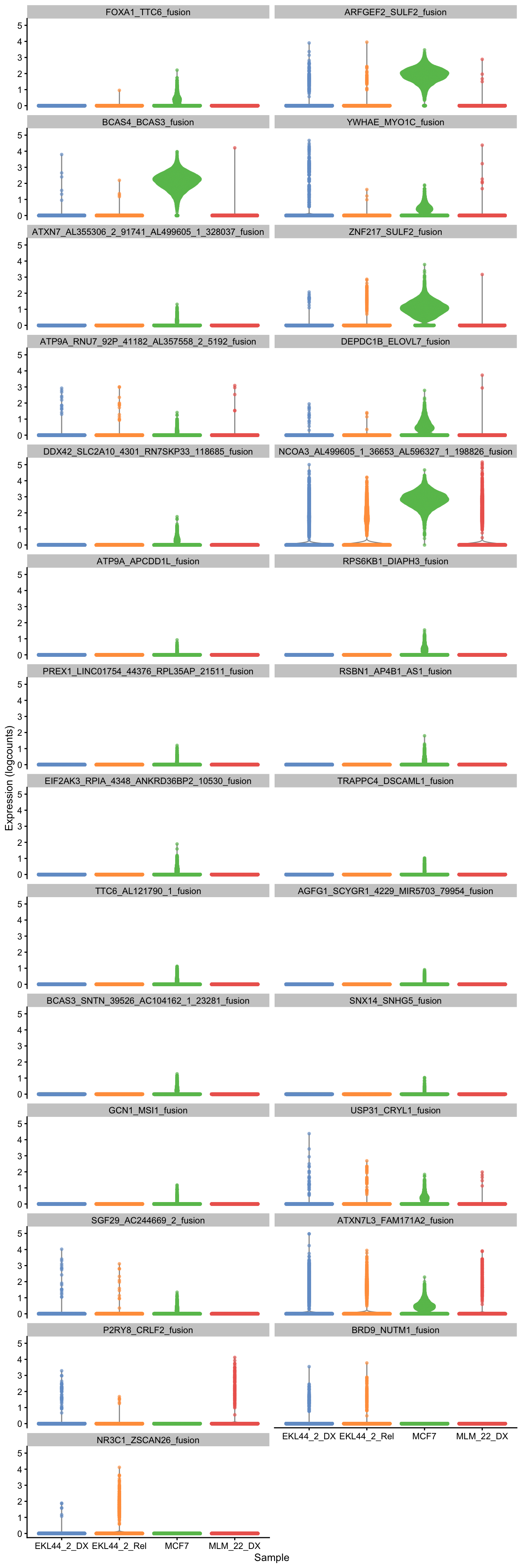

Past versions of plot-fusion-expression-post-filter-1.png

Version	Author	Date
1b5bb97	Jovana Maksimovic	2026-05-11

sce_fusions_post_qc <- sub[row.names(sce_fusions)]

fusion_output_post_qc <- rowSums(counts(sce_fusions_post_qc)) %>% 
  as.data.frame %>%
  rownames_to_column(var = "Fusion") %>%
  dplyr::rename("Total counts" = ".") %>% knitr::kable()
fusion_output_post_qc

Fusion	Total counts
FOXA1_TTC6_fusion	4002
ARFGEF2_SULF2_fusion	80401
BCAS4_BCAS3_fusion	100748
YWHAE_MYO1C_fusion	7216
ATXN7_AL355306_2_91741_AL499605_1_328037_fusion	805
ZNF217_SULF2_fusion	32542
ATP9A_RNU7_92P_41182_AL357558_2_5192_fusion	978
DEPDC1B_ELOVL7_fusion	11675
DDX42_SLC2A10_4301_RN7SKP33_118685_fusion	2880
NCOA3_AL499605_1_36653_AL596327_1_198826_fusion	179201
ATP9A_APCDD1L_fusion	81
RPS6KB1_DIAPH3_fusion	3404
PREX1_LINC01754_44376_RPL35AP_21511_fusion	572
RSBN1_AP4B1_AS1_fusion	1642
EIF2AK3_RPIA_4348_ANKRD36BP2_10530_fusion	1649
TRAPPC4_DSCAML1_fusion	576
TTC6_AL121790_1_fusion	1020
AGFG1_SCYGR1_4229_MIR5703_79954_fusion	281
BCAS3_SNTN_39526_AC104162_1_23281_fusion	1363
SNX14_SNHG5_fusion	131
GCN1_MSI1_fusion	308
USP31_CRYL1_fusion	4114
SGF29_AC244669_2_fusion	1215
ATXN7L3_FAM171A2_fusion	10629
P2RY8_CRLF2_fusion	188
BRD9_NUTM1_fusion	236
NR3C1_ZSCAN26_fusion	320

fusion_output

Fusion	Total counts
FOXA1_TTC6_fusion	4153
ARFGEF2_SULF2_fusion	83291
BCAS4_BCAS3_fusion	103456
YWHAE_MYO1C_fusion	7451
ATXN7_AL355306_2_91741_AL499605_1_328037_fusion	832
ZNF217_SULF2_fusion	33638
ATP9A_RNU7_92P_41182_AL357558_2_5192_fusion	1030
DEPDC1B_ELOVL7_fusion	11894
DDX42_SLC2A10_4301_RN7SKP33_118685_fusion	2967
NCOA3_AL499605_1_36653_AL596327_1_198826_fusion	187669
ATP9A_APCDD1L_fusion	82
RPS6KB1_DIAPH3_fusion	3491
PREX1_LINC01754_44376_RPL35AP_21511_fusion	588
RSBN1_AP4B1_AS1_fusion	1682
EIF2AK3_RPIA_4348_ANKRD36BP2_10530_fusion	1710
TRAPPC4_DSCAML1_fusion	608
TTC6_AL121790_1_fusion	1074
AGFG1_SCYGR1_4229_MIR5703_79954_fusion	299
BCAS3_SNTN_39526_AC104162_1_23281_fusion	1404
SNX14_SNHG5_fusion	136
GCN1_MSI1_fusion	317
USP31_CRYL1_fusion	4241
SGF29_AC244669_2_fusion	1259
ATXN7L3_FAM171A2_fusion	10969
P2RY8_CRLF2_fusion	197
BRD9_NUTM1_fusion	240
NR3C1_ZSCAN26_fusion	327

Doublet detection

Doublets are identified using scDblFinder. A UMAP is computed on the full (unfiltered) object to visualise doublet distribution across samples. Doublets are excluded from downstream analysis unless they carry a patient-specific fusion transcript, in which case the fusion assignment is retained.

out_doublets <- here("data", "RDS", "exp1_doublets.sce.rds")

if(!file.exists(out_doublets)){
sub <- scDblFinder::scDblFinder(sub,
                                dbr.sd = 1,
                                BPPARAM = BiocParallel::MulticoreParam(3))
  saveRDS(sub, out_doublets)
} else {
  sub <- readRDS(out_doublets)
}

seu <- CreateSeuratObject(counts = counts(sub),
                          meta.data = colData(sub) %>% data.frame)
seu

An object of class Seurat 
37170 features across 35258 samples within 1 assay 
Active assay: RNA (37170 features, 0 variable features)
 1 layer present: counts

UMAP by sample

seu <- NormalizeData(seu)
seu <- FindVariableFeatures(seu, selection.method = "vst",
                                  nfeatures = 3000, verbose = FALSE)
seu <- ScaleData(seu)
seu <- RunPCA(seu, verbose = FALSE, npcs = 30)
seu <- RunUMAP(seu, dims = 1:30, reduction = "pca")

DimPlot(seu, reduction = "umap", group.by = "Sample")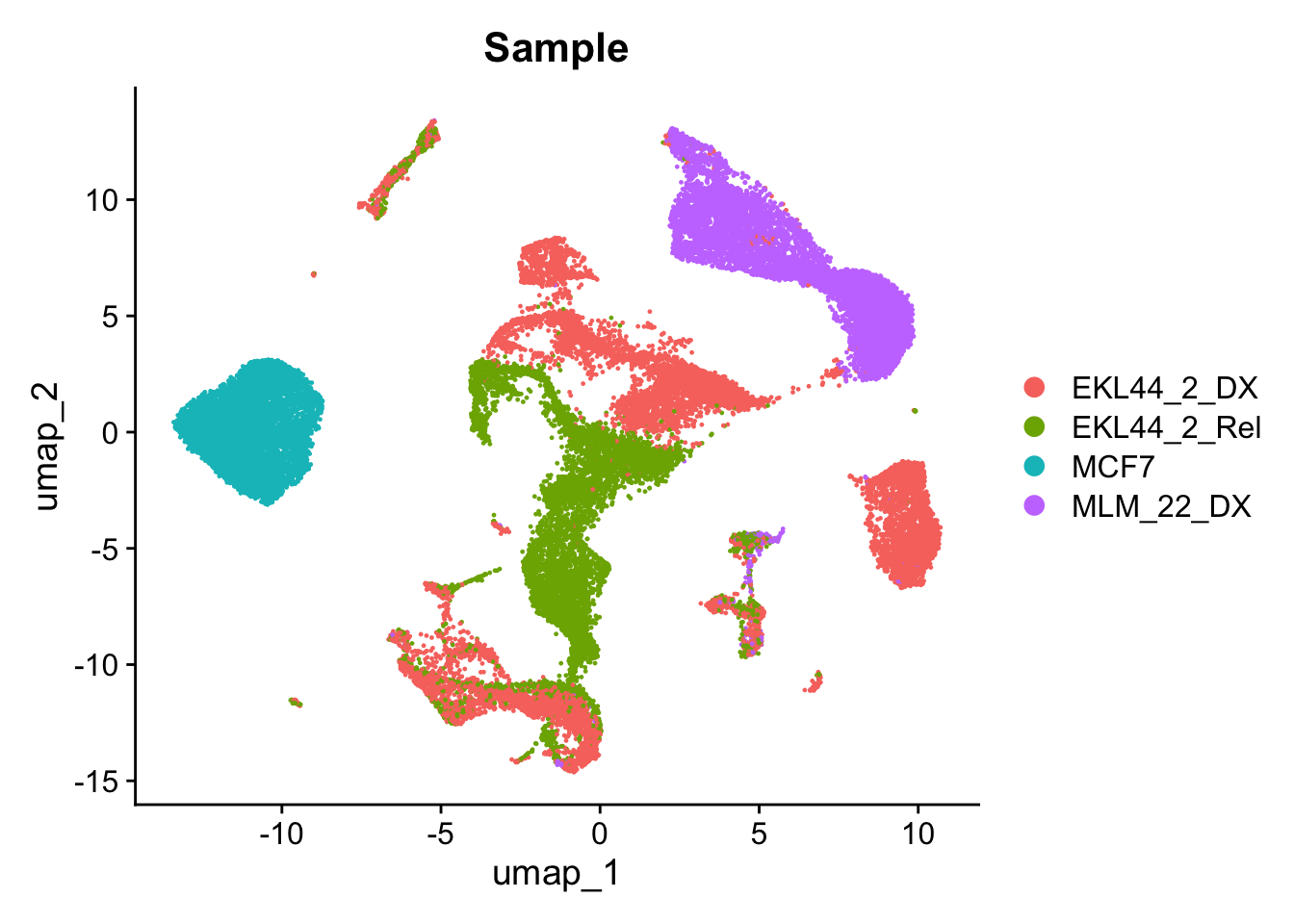

Past versions of plot-umap-1.png

Version	Author	Date
1b5bb97	Jovana Maksimovic	2026-05-11

DimPlot(seu, reduction = "umap", group.by = "scDblFinder.class")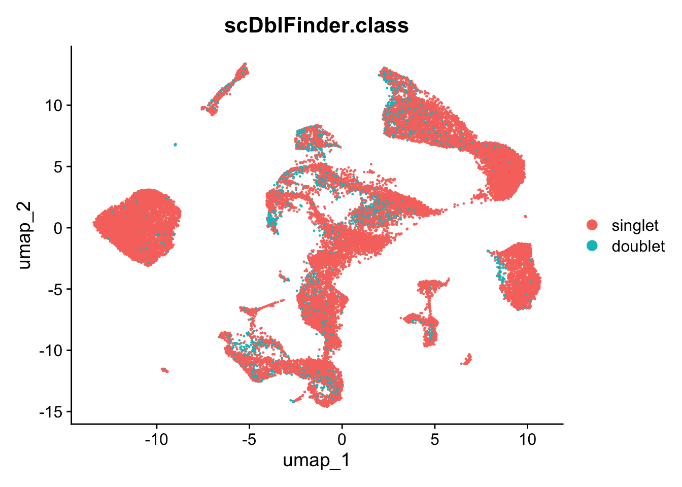

Past versions of plot-umap-2.png

Version	Author	Date
1b5bb97	Jovana Maksimovic	2026-05-11

Doublets per sample

seu@meta.data %>%
ggplot(aes(x = Sample, fill = scDblFinder.class)) +
  geom_bar() +
  ylab("Number of droplets") +
  theme(axis.text.x = element_text(angle = 45, hjust = 1)) +
  facet_grid(Sample ~ ., scales = "free_y") +
  theme_bw()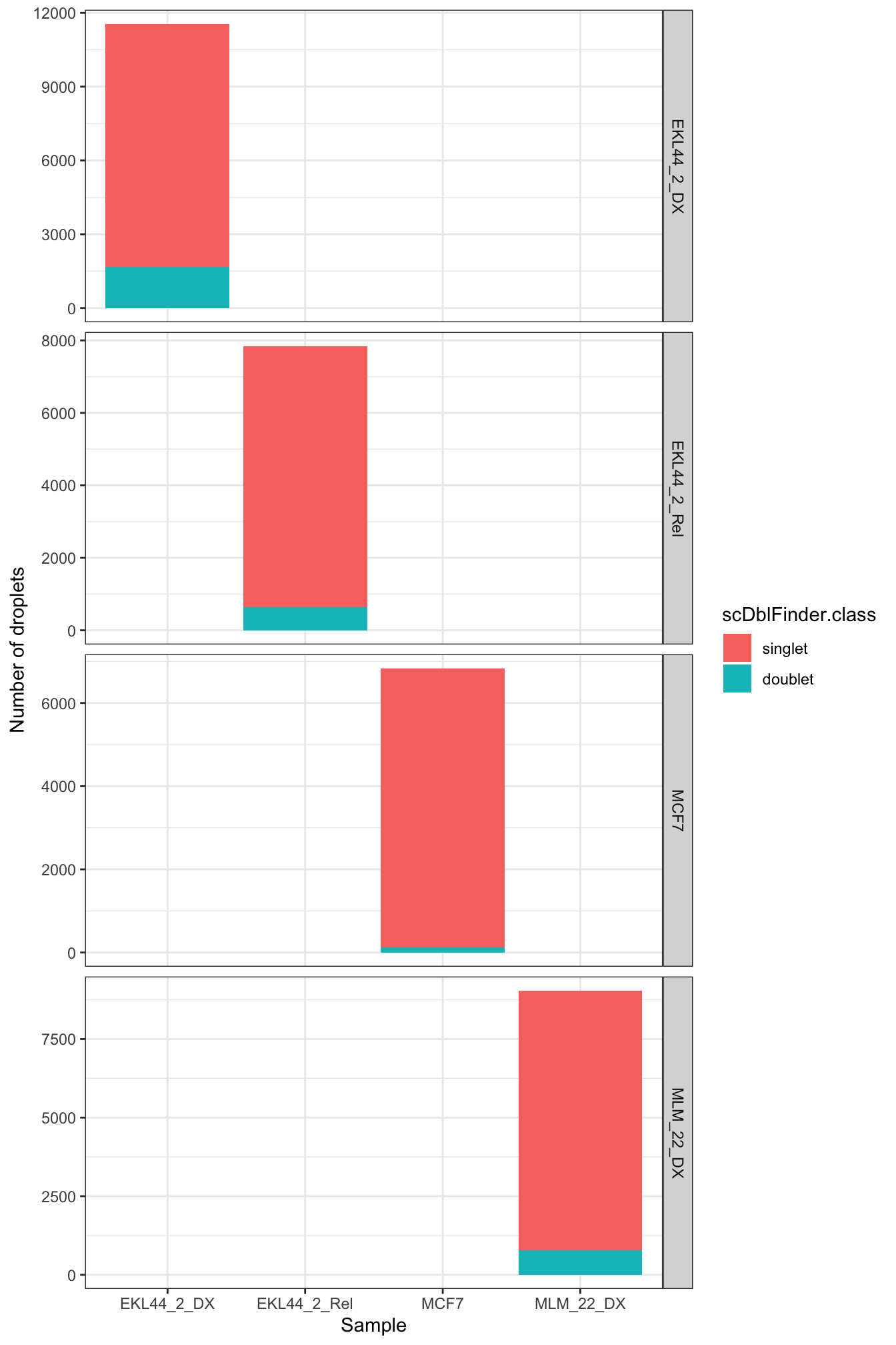

Past versions of plot-doublets-1.png

Version	Author	Date
1b5bb97	Jovana Maksimovic	2026-05-11

Filter singlets

sce_singlets <- sub[, sub$scDblFinder.class == "singlet"]
sce_singlets

class: SingleCellExperiment 
dim: 37170 32038 
metadata(2): Samples scDblFinder.threshold
assays(2): counts logcounts
rownames(37170): ENSG00000243485 ENSG00000237613 ...
  DEPRECATED_ENSG00000284873 DEPRECATED_ENSG00000285687
rowData names(6): ID Symbol ... subsets_is_mito scDblFinder.selected
colnames(32038): AAACAAGCAACAAGTTAGTAGGCT-1 AAACAAGCAAGAACAAACTTTAGG-1
  ... TTTGTGAGTTGCTCCTAACGGGAA-1 TTTGTGAGTTGCTCCTACTTTAGG-1
colData names(18): Sample Barcode ... scDblFinder.weighted
  scDblFinder.cxds_score
reducedDimNames(0):
mainExpName: NULL
altExpNames(0):

Filter high library size outliers

Even after doublet removal, a small number of cells with extreme total UMI counts remain. These likely represent higher-order multiplets (triplets or greater) that scDblFinder did not flag. Upper-bound outliers are identified per sample at 4 MADs above the median on the log scale.

umi_drop_upper <- isOutlier(
  metric = sce_singlets$sum,
  nmads  = 4,
  type   = "higher",
  log    = TRUE,
  batch  = sce_singlets$Sample)

data.frame(
  sample    = colnames(attributes(umi_drop_upper)$thresholds),
  threshold = attributes(umi_drop_upper)$thresholds["higher", ],
  row.names = NULL
) %>%
  left_join(
    colData(sce_singlets) %>% data.frame() %>%
      group_by(Sample) %>%
      summarise(P999 = quantile(sum, 0.999), Max = max(sum)),
    by = c("sample" = "Sample")
  ) %>%
  knitr::kable(row.names = FALSE,
               caption = "Upper UMI thresholds vs P99.9 and Max per sample")

Upper UMI thresholds vs P99.9 and Max per sample

sample	threshold	P999	Max
EKL44_2_DX	89927.58	32269.19	50797
EKL44_2_Rel	40622.19	22878.73	90352
MCF7	499385.09	232757.96	323883
MLM_22_DX	39319.03	11817.11	32599

data.frame(drop = umi_drop_upper, sample = sce_singlets$Sample) %>%
  group_by(sample) %>%
  summarise(Drop = sum(drop), Keep = n() - sum(drop)) %>%
  knitr::kable(row.names = FALSE,
               caption = "Cells removed by upper UMI filter after doublet removal")

Cells removed by upper UMI filter after doublet removal

sample	Drop	Keep
EKL44_2_DX	0	9880
EKL44_2_Rel	1	7194
MCF7	0	6709
MLM_22_DX	0	8254

sce_qc <- sce_singlets[, !umi_drop_upper]
sce_qc

class: SingleCellExperiment 
dim: 37170 32037 
metadata(2): Samples scDblFinder.threshold
assays(2): counts logcounts
rownames(37170): ENSG00000243485 ENSG00000237613 ...
  DEPRECATED_ENSG00000284873 DEPRECATED_ENSG00000285687
rowData names(6): ID Symbol ... subsets_is_mito scDblFinder.selected
colnames(32037): AAACAAGCAACAAGTTAGTAGGCT-1 AAACAAGCAAGAACAAACTTTAGG-1
  ... TTTGTGAGTTGCTCCTAACGGGAA-1 TTTGTGAGTTGCTCCTACTTTAGG-1
colData names(18): Sample Barcode ... scDblFinder.weighted
  scDblFinder.cxds_score
reducedDimNames(0):
mainExpName: NULL
altExpNames(0):

Note on Supplementary Figure 2 panels

The cell-recovery and QC-violin panels for Supplementary Figure 2 (panels A–B) now live in B-ALL_exp1_clustering.Rmd, which reads exp1_qc.sce.rds directly. This keeps all Supplementary Figure 2 panels — QC summary (A, B) and per-sample clustering grid (C) — in one notebook. This notebook is responsible only for the QC filtering that produces exp1_qc.sce.rds.

Save outputs

out <- here("data", "RDS", "exp1_qc.sce.rds")
saveRDS(sce_qc, out)
fs::file_chmod(out, "664")
try(fs::file_chown(out, group_id = "oshlack_lab"),
    silent = TRUE)

MCF7 ambient fusion contamination

Because MCF7 and B-ALL samples were co-multiplexed in the same capture, MCF7 fusion probe-RNA complexes may be captured by B-ALL cells as ambient contamination. This section quantifies the rate of MCF7 fusion detection in B-ALL cells and characterises the contamination profile by UMI count distribution and library size.

This analysis produces Supplementary Figure 3.

# Subset to QC-filtered singlet cells
unique(sce_qc$Sample)

[1] EKL44_2_DX  MCF7        EKL44_2_Rel MLM_22_DX  
Levels: EKL44_2_DX EKL44_2_Rel MCF7 MLM_22_DX

# ── Retrieve MCF7-specific fusions ───────────────────────────────────────────
ball_fusions <- c("P2RY8_CRLF2_fusion", "NR3C1_ZSCAN26_fusion", "BRD9_NUTM1_fusion")
all_fusions  <- rownames(sce_qc)[grepl("_fusion$", rownames(sce_qc))]
mcf7_fusions <- setdiff(all_fusions, ball_fusions)

ball_samples <- c("EKL44_2_DX", "EKL44_2_Rel", "MLM_22_DX")
ball_cells   <- colnames(sce_qc)[sce_qc$Sample %in% ball_samples]

mcf7_counts  <- counts(sce_qc)[mcf7_fusions, ball_cells]

ball_meta <- as.data.frame(colData(sce_qc)) %>%
  tibble::rownames_to_column("cell") %>%
  filter(Sample %in% ball_samples) %>%
  select(cell, Sample)

# ── Contamination summary ─────────────────────────────────────────────────────
contamination_df_filtered <- lapply(mcf7_fusions, function(fn) {
  counts_vec <- as.numeric(mcf7_counts[fn, ball_meta$cell])
  ball_meta %>%
    mutate(
      detected = counts_vec > 0,
      umi      = counts_vec
    ) %>%
    group_by(Sample) %>%
    summarise(
      n_cells      = n(),
      n_detected   = sum(detected),
      pct_detected = mean(detected) * 100,
      median_umi   = ifelse(any(detected), median(umi[detected]), NA_real_),
      .groups      = "drop"
    ) %>%
    mutate(fusion = fn)
}) %>%
  bind_rows() %>%
  arrange(Sample, desc(pct_detected))

# ── Compare pre vs post doublet removal ───────────────────────────────────────
contamination_df_filtered %>%
  group_by(Sample) %>%
  summarise(
    total_detections  = sum(n_detected),
    mean_pct_detected = mean(pct_detected),
    max_pct_detected  = max(pct_detected),
    .groups           = "drop"
  )

# A tibble: 3 × 4
  Sample      total_detections mean_pct_detected max_pct_detected
  <fct>                  <int>             <dbl>            <dbl>
1 EKL44_2_DX              1677             0.707             8.40
2 EKL44_2_Rel             1974             1.14             17.1 
3 MLM_22_DX                862             0.435             8.34

contamination_df_filtered %>% filter(pct_detected > 0)

# A tibble: 29 × 6
   Sample     n_cells n_detected pct_detected median_umi fusion                 
   <fct>        <int>      <int>        <dbl>      <dbl> <chr>                  
 1 EKL44_2_DX    9880        830       8.40            1 NCOA3_AL499605_1_36653…
 2 EKL44_2_DX    9880        499       5.05            1 ATXN7L3_FAM171A2_fusion
 3 EKL44_2_DX    9880        162       1.64            1 YWHAE_MYO1C_fusion     
 4 EKL44_2_DX    9880        112       1.13            1 ARFGEF2_SULF2_fusion   
 5 EKL44_2_DX    9880         22       0.223           1 USP31_CRYL1_fusion     
 6 EKL44_2_DX    9880         15       0.152           1 SGF29_AC244669_2_fusion
 7 EKL44_2_DX    9880         12       0.121           1 ZNF217_SULF2_fusion    
 8 EKL44_2_DX    9880         11       0.111           1 ATP9A_RNU7_92P_41182_A…
 9 EKL44_2_DX    9880         10       0.101           1 DEPDC1B_ELOVL7_fusion  
10 EKL44_2_DX    9880          4       0.0405          1 BCAS4_BCAS3_fusion     
# ℹ 19 more rows

Four-panel figure assembled with patchwork: (A) pseudobulk fusion count (log2) per MCF7-specific probe across all four Exp1 samples (MCF7, MLM_22_DX, EKL44_2_DX, EKL44_2_Rel), bars coloured by probe GC content; (B) UMI count distribution of all MCF7 ambient detections; (C) library size by any MCF7 fusion detection status (Wilcoxon test); (D) heatmap of contamination rates across all MCF7 fusions and samples.

# Supplementary Figure 3: MCF7 ambient fusion contamination in B-ALL samples
# ── Setup ─────────────────────────────────────────────────────────────────────
ball_fusions <- c("P2RY8_CRLF2_fusion", "NR3C1_ZSCAN26_fusion", "BRD9_NUTM1_fusion")
all_fusions  <- rownames(sce_qc)[grepl("_fusion$", rownames(sce_qc))]
mcf7_fusions <- setdiff(all_fusions, ball_fusions)
ball_samples <- c("EKL44_2_DX", "EKL44_2_Rel", "MLM_22_DX")
ball_cells <- colnames(sce_qc)[sce_qc$Sample %in% ball_samples]
mcf7_counts <- counts(sce_qc)[mcf7_fusions, ball_cells]

ball_meta_full <- as.data.frame(colData(sce_qc)) %>%
  tibble::rownames_to_column("cell") %>%
  filter(Sample %in% ball_samples)

ball_meta <- ball_meta_full %>% select(cell, Sample)

# ── Contamination df ──────────────────────────────────────────────────────────
contamination_df <- lapply(mcf7_fusions, function(fn) {
  counts_vec <- as.numeric(mcf7_counts[fn, ball_meta$cell])
  ball_meta %>%
    mutate(
      detected = counts_vec > 0,
      umi      = counts_vec
    ) %>%
    group_by(Sample) %>%
    summarise(
      n_cells      = n(),
      n_detected   = sum(detected),
      pct_detected = mean(detected) * 100,
      median_umi   = ifelse(any(detected), median(umi[detected]), NA_real_),
      .groups      = "drop"
    ) %>%
    mutate(fusion = fn)
}) %>%
  bind_rows() %>%
  arrange(Sample, desc(pct_detected))

# ── Library size and Wilcoxon test ────────────────────────────────────────────
# Flag cells with any MCF7 fusion detection
ball_meta_full$any_fusion_detected <- colSums(
  mcf7_counts[, ball_meta_full$cell, drop = FALSE]
) > 0

ball_meta_full$total_counts <- colSums(
  counts(sce_qc)[, ball_meta_full$cell]
)

wt <- wilcox.test(
  ball_meta_full$total_counts[ball_meta_full$any_fusion_detected],
  ball_meta_full$total_counts[!ball_meta_full$any_fusion_detected]
)

clean_fusion_label <- function(x) {
  x %>%
    gsub("_fusion$", "", .) %>%
    gsub("_", "::", ., fixed = TRUE) %>%
    gsub("(\\w+::\\w+)::.*", "\\1", .)
}

# ── Panel A: Pseudobulk fusion count coloured by probe GC content ─────────────
# Load probe GC content from mcf7_fusion_stats (average of both probe halves)
probe_stats <- readRDS(here("data", "RDS", "mcf7_fusion_stats.rds")) %>%
  { if (!"fusion_id" %in% colnames(.)) tibble::rownames_to_column(., "fusion_id") else . } %>%
  mutate(
    average_gc   = (GC_first_half + GC_second_half) / 2,
    # stats uses hyphen-separated names; SCE features use underscores
    feature_name = gsub("-", "_", fusion_id)
  ) %>%
  select(feature_name, average_gc)

# Compute pseudobulk counts across all 4 Exp1 samples
exp1_samples <- c("MCF7", "MLM_22_DX", "EKL44_2_DX", "EKL44_2_Rel")

pseudobulk_df <- lapply(exp1_samples, function(samp) {
  cells   <- colnames(sce_qc)[sce_qc$Sample == samp]
  cnt_mat <- counts(sce_qc)[mcf7_fusions, cells, drop = FALSE]
  data.frame(
    feature_name = mcf7_fusions,
    pseudobulk   = rowSums(cnt_mat),
    sample       = samp,
    stringsAsFactors = FALSE
  )
}) %>%
  bind_rows() %>%
  left_join(probe_stats, by = "feature_name") %>%
  mutate(
    log2_count = log2(pseudobulk + 1),
    sample     = factor(sample, levels = exp1_samples)
  )

# Order probes by MCF7 pseudobulk count (ascending so highest probe sits at top)
probe_order <- pseudobulk_df %>%
  filter(sample == "MCF7") %>%
  arrange(pseudobulk) %>%
  pull(feature_name)

pseudobulk_df <- pseudobulk_df %>%
  mutate(feature_name = factor(feature_name, levels = probe_order))

p_A <- ggplot(pseudobulk_df %>% filter(log2_count > 0),
              aes(x = log2_count, y = feature_name, fill = average_gc)) +
  geom_col(width = 0.7) +
  facet_wrap(~ sample, nrow = 1, scales = "free_x") +
  scale_fill_viridis_c(
    name   = "Probe GC content",
    limits = c(0.44, 0.68),
    option = "viridis"
  ) +
  scale_x_continuous(expand = expansion(mult = c(0, 0.05))) +
  scale_y_discrete(labels = clean_fusion_label) +
  labs(
    x     = "Pseudobulk fusion count (log2)",
    y     = "MCF7-specific fusion probe",
    title = "Pseudobulk fusion count per MCF7 probe"
  ) +
  theme_classic(base_size = 9) +
  theme(
    plot.title         = element_text(size = 10, face = "bold", colour = "grey15"),
    axis.text.y        = element_text(size =  7, colour = "grey20"),
    axis.text.x        = element_text(size =  7, colour = "grey20"),
    axis.title         = element_text(size =  9, colour = "grey20"),
    strip.background   = element_blank(),
    strip.text         = element_text(size =  9, face = "bold", colour = "grey15"),
    panel.grid.major.x = element_line(colour = "grey92", linewidth = 0.3),
    panel.spacing.x    = unit(0.5, "cm"),
    legend.position    = "bottom",
    legend.title       = element_text(size = 8),
    legend.text        = element_text(size = 8),
    legend.key.width   = unit(1.5, "cm")
  )

# ── Panel B: UMI distribution ─────────────────────────────────────────────────
all_ambient_umis <- mcf7_fusions %>%
  lapply(function(fn) {
    counts_vec <- as.numeric(counts(sce_qc)[fn, ball_meta_full$cell])
    counts_vec[counts_vec > 0]
  }) %>%
  unlist(use.names = FALSE)

umi_dist <- data.frame(umi = all_ambient_umis) %>%
  dplyr::count(umi) %>%
  mutate(pct = n / sum(n) * 100)

p_B <- ggplot(umi_dist, aes(x = factor(umi), y = pct)) +
  geom_col(fill = "#56B4E9", width = 0.6) +
  geom_text(aes(label = paste0(round(pct, 1), "%")),
            vjust = -0.5, size = 2.8, colour = "grey30") +
  scale_y_continuous(expand = expansion(mult = c(0, 0.12))) +
  labs(x = "Fusion UMI count", y = "% of detections",
       title = "UMI distribution of MCF7 ambient detections") +
  theme_classic(base_size = 10) +
  theme(
    plot.title         = element_text(size = 10, face = "bold", colour = "grey15"),
    axis.text          = element_text(size = 8, colour = "grey15"),
    panel.grid.major.y = element_line(colour = "grey92", linewidth = 0.3)
  )

# ── Panel C: Library size vs any MCF7 fusion detection ────────────────────────
p_C <- ball_meta_full %>%
  mutate(
    detection = ifelse(any_fusion_detected, "Fusion+", "Fusion−"),
    Sample    = factor(Sample, levels = c("MLM_22_DX", "EKL44_2_DX", "EKL44_2_Rel"))
  ) %>%
  ggplot(aes(x = detection, y = total_counts, fill = detection)) +
  geom_violin(scale = "width", alpha = 0.8) +
  geom_boxplot(width = 0.15, fill = "white", outlier.size = 0.3,
               colour = "grey30") +
  scale_fill_manual(values = c("Fusion+"  = "#D55E00",
                               "Fusion−" = "grey70")) +
  scale_y_log10(labels = scales::comma) +
  facet_wrap(~Sample, nrow = 1) +
  labs(x = NULL, y = "Total UMI count (log scale)",
       title = "Library size by any MCF7 fusion detection") +
  theme_classic(base_size = 10) +
  theme(
    plot.title         = element_text(size = 10, face = "bold", colour = "grey15"),
    axis.text          = element_text(size = 8, colour = "grey15"),
    panel.grid.major.y = element_line(colour = "grey92", linewidth = 0.3),
    strip.background   = element_blank(),
    strip.text         = element_text(size = 9, face = "bold", colour = "grey15"),
    legend.position    = "none"
  ) +
  geom_text(
    data = data.frame(
      Sample = factor("MLM_22_DX",
                      levels = c("MLM_22_DX", "EKL44_2_DX", "EKL44_2_Rel")),
      x      = 1.5,
      y      = 55000,
      label  = paste0("Wilcoxon p = ", format(wt$p.value, scientific = TRUE, digits = 2))
    ),
    aes(x = x, y = y, label = label),
    inherit.aes = FALSE,
    size        = 2.5,
    colour      = "grey30",
    fontface    = "italic"
  )

# ── Panel D: Heatmap — all MCF7 fusions ──────────────────────────────────────
all_fusion_order <- contamination_df %>%
  group_by(fusion) %>%
  summarise(max_pct = max(pct_detected), .groups = "drop") %>%
  arrange(desc(max_pct)) %>%
  pull(fusion)

p_D <- contamination_df %>%
  mutate(
    fusion_label = clean_fusion_label(fusion),
    fusion_label = factor(fusion_label,
                          levels = rev(clean_fusion_label(all_fusion_order))),
    Sample = factor(Sample, levels = c("MLM_22_DX", "EKL44_2_DX", "EKL44_2_Rel"))
  ) %>%
  ggplot(aes(x = Sample, y = fusion_label, fill = pct_detected)) +
  geom_tile(colour = "white", linewidth = 0.5) +
  geom_text(aes(label = ifelse(pct_detected > 0, round(pct_detected, 2), "")),
            size = 2.5, colour = "grey15") +
  scale_fill_gradient(
    low  = "white",
    high = "#D55E00",
    name = "% cells\ndetected"
  ) +
  labs(x = NULL, y = NULL,
       title = "MCF7 fusion contamination rates (%)") +
  theme_classic(base_size = 10) +
  theme(
    plot.title   = element_text(size = 10, face = "bold", colour = "grey15"),
    axis.text.x  = element_text(size = 8, colour = "grey15", angle = 30, hjust = 1),
    axis.text.y  = element_text(size = 7, colour = "grey15"),
    legend.text  = element_text(size = 8),
    legend.title = element_text(size = 8)
  )

# ── Assemble ──────────────────────────────────────────────────────────────────
# Panel A (wide 4-facet) on left; B, C, D stacked on right
# wrap_elements() prevents patchwork axis alignment from pushing titles away from plots
# B is compact, D (heatmap) gets most of the right column height
# Tag theme is applied to each panel individually (matching Figure 3 / Supp Fig 2) —
# patchwork reads plot.tag from each panel's own theme, so setting it only in the
# final plot_annotation() theme is unreliable and the size/face don't take effect.
tag_theme <- theme(plot.tag = element_text(size = 18, face = "bold"))

pA_tagged <- wrap_elements(p_A) + tag_theme
pB_tagged <- wrap_elements(p_B) + tag_theme
pC_tagged <- wrap_elements(p_C) + tag_theme
pD_tagged <- p_D + tag_theme

right_col <- (pB_tagged / pC_tagged / pD_tagged) +
  plot_layout(heights = c(0.8, 1, 2))
(pA_tagged | right_col) +
  plot_layout(widths = c(2.5, 1.25)) +
  plot_annotation(tag_levels = "A")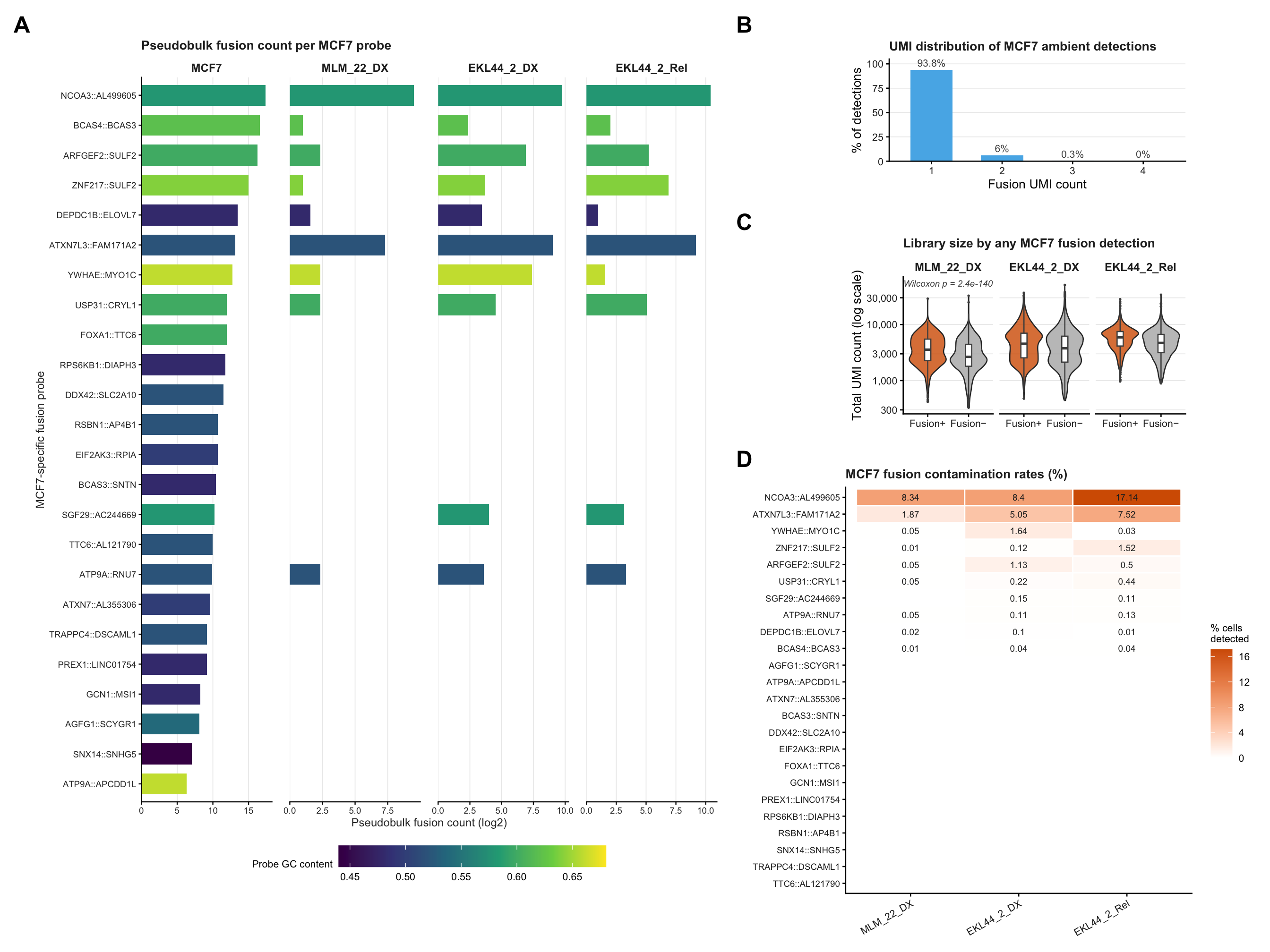

Past versions of fig-mcf7-contamination-1.png

Version	Author	Date
1b5bb97	Jovana Maksimovic	2026-05-11

Session info

The analysis and this document were prepared using the following software (click triangle to expand)

sessioninfo::session_info()

─ Session info ───────────────────────────────────────────────────────────────
 setting  value
 version  R version 4.4.1 (2024-06-14)
 os       macOS 15.5
 system   aarch64, darwin20
 ui       X11
 language (EN)
 collate  en_US.UTF-8
 ctype    en_US.UTF-8
 tz       Australia/Melbourne
 date     2026-07-15
 pandoc   3.8.3 @ /Applications/RStudio.app/Contents/Resources/app/quarto/bin/tools/aarch64/ (via rmarkdown)
 quarto   1.9.38 @ /Applications/RStudio.app/Contents/Resources/app/quarto/bin/quarto

─ Packages ───────────────────────────────────────────────────────────────────
 ! package              * version   date (UTC) lib source
 P abind                  1.4-8     2024-09-12 [?] CRAN (R 4.4.1)
 P beachmat               2.22.0    2024-11-08 [?] Bioconduc~
 P beeswarm               0.4.0     2021-06-01 [?] CRAN (R 4.4.1)
 P Biobase              * 2.66.0    2024-11-08 [?] Bioconduc~
 P BiocGenerics         * 0.52.0    2024-11-08 [?] Bioconduc~
 P BiocIO                 1.16.0    2024-11-08 [?] Bioconduc~
 P BiocManager            1.30.27   2025-11-14 [?] CRAN (R 4.4.3)
 P BiocNeighbors          2.0.1     2024-11-28 [?] Bioconduc~
 P BiocParallel           1.40.2    2025-04-08 [?] Bioconductor
 P BiocSingular           1.22.0    2024-11-08 [?] Bioconduc~
 P Biostrings             2.74.1    2024-12-16 [?] Bioconduc~
 P bitops                 1.0-9     2024-10-03 [?] CRAN (R 4.4.1)
 P bluster                1.16.0    2024-11-08 [?] Bioconduc~
 P bslib                  0.9.0     2025-01-30 [?] CRAN (R 4.4.1)
 P cachem                 1.1.0     2024-05-16 [?] CRAN (R 4.4.1)
 P callr                  3.7.6     2024-03-25 [?] CRAN (R 4.4.0)
 P cli                    3.6.5     2025-04-23 [?] CRAN (R 4.4.1)
 P cluster                2.1.6     2023-12-01 [?] CRAN (R 4.4.1)
 P codetools              0.2-20    2024-03-31 [?] CRAN (R 4.4.1)
 P colorspace             2.1-1     2024-07-26 [?] CRAN (R 4.4.1)
 P cowplot                1.1.3     2024-01-22 [?] CRAN (R 4.4.0)
 P crayon                 1.5.3     2024-06-20 [?] CRAN (R 4.4.1)
 P curl                   6.2.3     2025-05-24 [?] CRAN (R 4.4.1)
 P data.table             1.18.2.1  2026-01-27 [?] CRAN (R 4.4.3)
 P DelayedArray           0.32.0    2024-11-08 [?] Bioconduc~
 P DelayedMatrixStats     1.28.1    2025-01-09 [?] Bioconduc~
 P deldir                 2.0-4     2024-02-28 [?] CRAN (R 4.4.1)
 P digest                 0.6.37    2024-08-19 [?] CRAN (R 4.4.1)
 P dotCall64              1.2       2024-10-04 [?] CRAN (R 4.4.1)
 P dplyr                * 1.1.4     2023-11-17 [?] CRAN (R 4.4.0)
 P dqrng                  0.4.1     2024-05-28 [?] CRAN (R 4.4.0)
 P DropletUtils         * 1.26.0    2024-11-08 [?] Bioconduc~
 P edgeR                  4.4.2     2025-01-27 [?] Bioconduc~
 P evaluate               1.0.3     2025-01-10 [?] CRAN (R 4.4.1)
 P farver                 2.1.2     2024-05-13 [?] CRAN (R 4.4.1)
 P fastDummies            1.7.5     2025-01-20 [?] CRAN (R 4.4.1)
 P fastmap                1.2.0     2024-05-15 [?] CRAN (R 4.4.1)
 P fitdistrplus           1.2-2     2025-01-07 [?] CRAN (R 4.4.1)
 P forcats              * 1.0.0     2023-01-29 [?] CRAN (R 4.4.0)
 P fs                     1.6.6     2025-04-12 [?] CRAN (R 4.4.1)
 P future                 1.49.0    2025-05-09 [?] CRAN (R 4.4.1)
 P future.apply           1.11.3    2024-10-27 [?] CRAN (R 4.4.1)
 P generics               0.1.4     2025-05-09 [?] CRAN (R 4.4.1)
 P GenomeInfoDb         * 1.42.3    2025-01-27 [?] Bioconduc~
 P GenomeInfoDbData       1.2.13    2025-05-28 [?] Bioconductor
 P GenomicAlignments      1.42.0    2024-11-08 [?] Bioconduc~
 P GenomicRanges        * 1.58.0    2024-11-08 [?] Bioconduc~
 P getPass                0.2-4     2023-12-10 [?] CRAN (R 4.4.1)
 P ggbeeswarm             0.7.2     2023-04-29 [?] CRAN (R 4.4.0)
 P ggplot2              * 4.0.2     2026-02-03 [?] CRAN (R 4.4.3)
 P ggrepel                0.9.6     2024-09-07 [?] CRAN (R 4.4.1)
 P ggridges               0.5.6     2024-01-23 [?] CRAN (R 4.4.0)
 P git2r                  0.36.2    2025-03-29 [?] CRAN (R 4.4.1)
 P globals                0.18.0    2025-05-08 [?] CRAN (R 4.4.1)
 P glue                 * 1.8.0     2024-09-30 [?] CRAN (R 4.4.1)
 P goftest                1.2-3     2021-10-07 [?] CRAN (R 4.4.1)
 P gridExtra              2.3       2017-09-09 [?] CRAN (R 4.4.1)
 P gtable                 0.3.6     2024-10-25 [?] CRAN (R 4.4.1)
 P HDF5Array              1.34.0    2024-11-08 [?] Bioconduc~
 P here                 * 1.0.1     2020-12-13 [?] CRAN (R 4.4.1)
 P hms                    1.1.3     2023-03-21 [?] CRAN (R 4.4.0)
 P htmltools              0.5.8.1   2024-04-04 [?] CRAN (R 4.4.1)
 P htmlwidgets            1.6.4     2023-12-06 [?] CRAN (R 4.4.0)
 P httpuv                 1.6.16    2025-04-16 [?] CRAN (R 4.4.1)
 P httr                   1.4.7     2023-08-15 [?] CRAN (R 4.4.0)
 P ica                    1.0-3     2022-07-08 [?] CRAN (R 4.4.1)
 P igraph                 2.1.4     2025-01-23 [?] CRAN (R 4.4.1)
 P IRanges              * 2.40.1    2024-12-05 [?] Bioconduc~
 P irlba                  2.3.5.1   2022-10-03 [?] CRAN (R 4.4.0)
 P jquerylib              0.1.4     2021-04-26 [?] CRAN (R 4.4.0)
 P jsonlite               2.0.0     2025-03-27 [?] CRAN (R 4.4.1)
 P KernSmooth             2.23-24   2024-05-17 [?] CRAN (R 4.4.1)
 P knitr                  1.50      2025-03-16 [?] CRAN (R 4.4.1)
 P labeling               0.4.3     2023-08-29 [?] CRAN (R 4.4.1)
 P later                  1.4.2     2025-04-08 [?] CRAN (R 4.4.1)
 P lattice                0.22-6    2024-03-20 [?] CRAN (R 4.4.1)
 P lazyeval               0.2.2     2019-03-15 [?] CRAN (R 4.4.1)
 P lifecycle              1.0.4     2023-11-07 [?] CRAN (R 4.4.1)
 P limma                  3.62.2    2025-01-09 [?] Bioconduc~
 P listenv                0.9.1     2024-01-29 [?] CRAN (R 4.4.1)
 P lmtest                 0.9-40    2022-03-21 [?] CRAN (R 4.4.1)
 P locfit                 1.5-9.12  2025-03-05 [?] CRAN (R 4.4.1)
 P lubridate            * 1.9.4     2024-12-08 [?] CRAN (R 4.4.1)
 P magrittr               2.0.3     2022-03-30 [?] CRAN (R 4.4.1)
 P MASS                   7.3-60.2  2024-04-26 [?] CRAN (R 4.4.1)
 P Matrix                 1.7-0     2024-04-26 [?] CRAN (R 4.4.1)
 P MatrixGenerics       * 1.18.1    2025-01-09 [?] Bioconduc~
 P matrixStats          * 1.5.0     2025-01-07 [?] CRAN (R 4.4.1)
 P metapod                1.14.0    2024-11-08 [?] Bioconduc~
 P mime                   0.13      2025-03-17 [?] CRAN (R 4.4.1)
 P miniUI                 0.1.2     2025-04-17 [?] CRAN (R 4.4.1)
 P nlme                   3.1-164   2023-11-27 [?] CRAN (R 4.4.1)
 P parallelly             1.45.0    2025-06-02 [?] CRAN (R 4.4.1)
 P patchwork            * 1.3.0     2024-09-16 [?] CRAN (R 4.4.1)
 P pbapply                1.7-4     2025-07-20 [?] CRAN (R 4.4.1)
 P pillar                 1.10.2    2025-04-05 [?] CRAN (R 4.4.1)
 P pkgconfig              2.0.3     2019-09-22 [?] CRAN (R 4.4.1)
 P plotly                 4.10.4    2024-01-13 [?] CRAN (R 4.4.0)
 P plyr                   1.8.9     2023-10-02 [?] CRAN (R 4.4.1)
 P png                    0.1-8     2022-11-29 [?] CRAN (R 4.4.1)
 P polyclip               1.10-7    2024-07-23 [?] CRAN (R 4.4.1)
 P processx               3.8.6     2025-02-21 [?] CRAN (R 4.4.1)
 P progressr              0.15.1    2024-11-22 [?] CRAN (R 4.4.1)
 P promises               1.3.3     2025-05-29 [?] CRAN (R 4.4.1)
 P ps                     1.9.1     2025-04-12 [?] CRAN (R 4.4.1)
 P purrr                * 1.0.4     2025-02-05 [?] CRAN (R 4.4.1)
 P R.methodsS3            1.8.2     2022-06-13 [?] CRAN (R 4.4.1)
 P R.oo                   1.27.1    2025-05-02 [?] CRAN (R 4.4.1)
 P R.utils                2.13.0    2025-02-24 [?] CRAN (R 4.4.1)
 P R6                     2.6.1     2025-02-15 [?] CRAN (R 4.4.1)
 P RANN                   2.6.2     2024-08-25 [?] CRAN (R 4.4.1)
 P RColorBrewer           1.1-3     2022-04-03 [?] CRAN (R 4.4.1)
 P Rcpp                   1.1.1-1.1 2026-04-24 [?] CRAN (R 4.4.1)
 P RcppAnnoy              0.0.22    2024-01-23 [?] CRAN (R 4.4.1)
 P RcppHNSW               0.6.0     2024-02-04 [?] CRAN (R 4.4.1)
 P RCurl                  1.98-1.17 2025-03-22 [?] CRAN (R 4.4.1)
 P readr                * 2.1.5     2024-01-10 [?] CRAN (R 4.4.0)
   renv                   1.1.4     2025-03-20 [1] CRAN (R 4.4.1)
 P reshape2               1.4.4     2020-04-09 [?] CRAN (R 4.4.0)
 P restfulr               0.0.15    2022-06-16 [?] CRAN (R 4.4.0)
 P reticulate             1.42.0    2025-03-25 [?] CRAN (R 4.4.1)
 P rhdf5                  2.50.2    2025-01-09 [?] Bioconduc~
 P rhdf5filters           1.18.1    2025-03-06 [?] Bioconduc~
 P Rhdf5lib               1.28.0    2024-11-08 [?] Bioconduc~
 P rjson                  0.2.23    2024-09-16 [?] CRAN (R 4.4.1)
 P rlang                  1.1.6     2025-04-11 [?] CRAN (R 4.4.1)
 P rmarkdown              2.29      2024-11-04 [?] CRAN (R 4.4.1)
 P ROCR                   1.0-11    2020-05-02 [?] CRAN (R 4.4.0)
 P rprojroot              2.0.4     2023-11-05 [?] CRAN (R 4.4.1)
 P Rsamtools              2.22.0    2024-11-08 [?] Bioconduc~
 P RSpectra               0.16-2    2024-07-18 [?] CRAN (R 4.4.0)
 P rstudioapi             0.17.1    2024-10-22 [?] CRAN (R 4.4.1)
 P rsvd                   1.0.5     2021-04-16 [?] CRAN (R 4.4.0)
 P rtracklayer            1.66.0    2024-11-08 [?] Bioconduc~
 P Rtsne                  0.17      2023-12-07 [?] CRAN (R 4.4.1)
 P S4Arrays               1.6.0     2024-11-08 [?] Bioconduc~
 P S4Vectors            * 0.44.0    2024-11-08 [?] Bioconduc~
 P S7                     0.2.0     2024-11-07 [?] CRAN (R 4.4.1)
 P sass                   0.4.10    2025-04-11 [?] CRAN (R 4.4.1)
 P ScaledMatrix           1.14.0    2024-11-08 [?] Bioconduc~
 P scales                 1.4.0     2025-04-24 [?] CRAN (R 4.4.1)
 P scater               * 1.34.1    2025-03-03 [?] Bioconduc~
 P scattermore            1.2       2023-06-12 [?] CRAN (R 4.4.0)
 P scDblFinder          * 1.20.2    2025-02-10 [?] Bioconduc~
 P scran                * 1.34.0    2024-11-08 [?] Bioconduc~
 P sctransform            0.4.2     2025-04-30 [?] CRAN (R 4.4.1)
 P scuttle              * 1.16.0    2024-11-08 [?] Bioconduc~
 P sessioninfo            1.2.3     2025-02-05 [?] CRAN (R 4.4.1)
 P Seurat               * 5.3.0     2025-04-23 [?] CRAN (R 4.4.1)
 P SeuratObject         * 5.1.0     2025-04-22 [?] CRAN (R 4.4.1)
 P shiny                  1.10.0    2024-12-14 [?] CRAN (R 4.4.1)
 P SingleCellExperiment * 1.28.1    2024-11-23 [?] Bioconduc~
 P sp                   * 2.2-0     2025-02-01 [?] CRAN (R 4.4.1)
 P spam                   2.11-1    2025-01-20 [?] CRAN (R 4.4.1)
 P SparseArray            1.6.2     2025-02-20 [?] Bioconduc~
 P sparseMatrixStats      1.18.0    2024-11-08 [?] Bioconduc~
 P spatstat.data          3.1-6     2025-03-17 [?] CRAN (R 4.4.1)
 P spatstat.explore       3.4-3     2025-05-21 [?] CRAN (R 4.4.1)
 P spatstat.geom          3.4-1     2025-05-20 [?] CRAN (R 4.4.1)
 P spatstat.random        3.4-1     2025-05-20 [?] CRAN (R 4.4.1)
 P spatstat.sparse        3.1-0     2024-06-21 [?] CRAN (R 4.4.0)
 P spatstat.univar        3.1-3     2025-05-08 [?] CRAN (R 4.4.1)
 P spatstat.utils         3.1-4     2025-05-15 [?] CRAN (R 4.4.1)
 P statmod                1.5.0     2023-01-06 [?] CRAN (R 4.4.1)
 P stringi                1.8.7     2025-03-27 [?] CRAN (R 4.4.1)
 P stringr              * 1.6.0     2025-11-04 [?] CRAN (R 4.4.1)
 P SummarizedExperiment * 1.36.0    2024-11-08 [?] Bioconduc~
 P survival               3.6-4     2024-04-24 [?] CRAN (R 4.4.1)
 P tensor                 1.5       2012-05-05 [?] CRAN (R 4.4.1)
 P tibble               * 3.2.1     2023-03-20 [?] CRAN (R 4.4.0)
 P tidyr                * 1.3.1     2024-01-24 [?] CRAN (R 4.4.1)
 P tidyselect             1.2.1     2024-03-11 [?] CRAN (R 4.4.0)
 P tidyverse            * 2.0.0     2023-02-22 [?] CRAN (R 4.4.0)
 P timechange             0.3.0     2024-01-18 [?] CRAN (R 4.4.1)
 P tzdb                   0.5.0     2025-03-15 [?] CRAN (R 4.4.1)
 P UCSC.utils             1.2.0     2024-11-08 [?] Bioconduc~
 P utf8                   1.2.5     2025-05-01 [?] CRAN (R 4.4.1)
 P uwot                   0.2.3     2025-02-24 [?] CRAN (R 4.4.1)
 P vctrs                  0.6.5     2023-12-01 [?] CRAN (R 4.4.0)
 P vipor                  0.4.7     2023-12-18 [?] CRAN (R 4.4.1)
 P viridis                0.6.5     2024-01-29 [?] CRAN (R 4.4.0)
 P viridisLite            0.4.2     2023-05-02 [?] CRAN (R 4.4.1)
 P whisker                0.4.1     2022-12-05 [?] CRAN (R 4.4.1)
 P withr                  3.0.2     2024-10-28 [?] CRAN (R 4.4.1)
 P workflowr            * 1.7.1     2023-08-23 [?] CRAN (R 4.4.0)
 P xfun                   0.56      2026-01-18 [?] CRAN (R 4.4.3)
 P xgboost                1.7.11.1  2025-05-15 [?] CRAN (R 4.4.1)
 P XML                    3.99-0.18 2025-01-01 [?] CRAN (R 4.4.1)
 P xtable                 1.8-4     2019-04-21 [?] CRAN (R 4.4.1)
 P XVector                0.46.0    2024-11-08 [?] Bioconduc~
 P yaml                   2.3.10    2024-07-26 [?] CRAN (R 4.4.1)
 P zlibbioc               1.52.0    2024-11-08 [?] Bioconduc~
 P zoo                    1.8-14    2025-04-10 [?] CRAN (R 4.4.1)

 [1] /Users/maksimovicjovana/Library/CloudStorage/OneDrive-PeterMac/Desktop/projects/my_research/flex-fusion-probes/renv/library/macos/R-4.4/aarch64-apple-darwin20
 [2] /Users/maksimovicjovana/Library/Caches/org.R-project.R/R/renv/sandbox/macos/R-4.4/aarch64-apple-darwin20/f7156815

 * ── Packages attached to the search path.
 P ── Loaded and on-disk path mismatch.

──────────────────────────────────────────────────────────────────────────────

Session information

sessionInfo()

R version 4.4.1 (2024-06-14)
Platform: aarch64-apple-darwin20
Running under: macOS 15.5

Matrix products: default
BLAS:   /Library/Frameworks/R.framework/Versions/4.4-arm64/Resources/lib/libRblas.0.dylib 
LAPACK: /Library/Frameworks/R.framework/Versions/4.4-arm64/Resources/lib/libRlapack.dylib;  LAPACK version 3.12.0

locale:
[1] en_US.UTF-8/en_US.UTF-8/en_US.UTF-8/C/en_US.UTF-8/en_US.UTF-8

time zone: Australia/Melbourne
tzcode source: internal

attached base packages:
[1] stats4    stats     graphics  grDevices datasets  utils     methods  
[8] base     

other attached packages:
 [1] scDblFinder_1.20.2          Seurat_5.3.0               
 [3] SeuratObject_5.1.0          sp_2.2-0                   
 [5] patchwork_1.3.0             scater_1.34.1              
 [7] scran_1.34.0                scuttle_1.16.0             
 [9] DropletUtils_1.26.0         SingleCellExperiment_1.28.1
[11] SummarizedExperiment_1.36.0 Biobase_2.66.0             
[13] GenomicRanges_1.58.0        GenomeInfoDb_1.42.3        
[15] IRanges_2.40.1              S4Vectors_0.44.0           
[17] BiocGenerics_0.52.0         MatrixGenerics_1.18.1      
[19] matrixStats_1.5.0           glue_1.8.0                 
[21] here_1.0.1                  lubridate_1.9.4            
[23] forcats_1.0.0               stringr_1.6.0              
[25] dplyr_1.1.4                 purrr_1.0.4                
[27] readr_2.1.5                 tidyr_1.3.1                
[29] tibble_3.2.1                ggplot2_4.0.2              
[31] tidyverse_2.0.0             workflowr_1.7.1            

loaded via a namespace (and not attached):
  [1] fs_1.6.6                  spatstat.sparse_3.1-0    
  [3] bitops_1.0-9              httr_1.4.7               
  [5] RColorBrewer_1.1-3        tools_4.4.1              
  [7] sctransform_0.4.2         utf8_1.2.5               
  [9] R6_2.6.1                  HDF5Array_1.34.0         
 [11] lazyeval_0.2.2            uwot_0.2.3               
 [13] rhdf5filters_1.18.1       withr_3.0.2              
 [15] gridExtra_2.3             progressr_0.15.1         
 [17] cli_3.6.5                 spatstat.explore_3.4-3   
 [19] fastDummies_1.7.5         labeling_0.4.3           
 [21] sass_0.4.10               S7_0.2.0                 
 [23] spatstat.data_3.1-6       ggridges_0.5.6           
 [25] pbapply_1.7-4             Rsamtools_2.22.0         
 [27] R.utils_2.13.0            sessioninfo_1.2.3        
 [29] parallelly_1.45.0         limma_3.62.2             
 [31] rstudioapi_0.17.1         generics_0.1.4           
 [33] BiocIO_1.16.0             ica_1.0-3                
 [35] spatstat.random_3.4-1     Matrix_1.7-0             
 [37] ggbeeswarm_0.7.2          abind_1.4-8              
 [39] R.methodsS3_1.8.2         lifecycle_1.0.4          
 [41] whisker_0.4.1             yaml_2.3.10              
 [43] edgeR_4.4.2               rhdf5_2.50.2             
 [45] SparseArray_1.6.2         Rtsne_0.17               
 [47] grid_4.4.1                promises_1.3.3           
 [49] dqrng_0.4.1               crayon_1.5.3             
 [51] miniUI_0.1.2              lattice_0.22-6           
 [53] beachmat_2.22.0           cowplot_1.1.3            
 [55] pillar_1.10.2             knitr_1.50               
 [57] metapod_1.14.0            rjson_0.2.23             
 [59] xgboost_1.7.11.1          future.apply_1.11.3      
 [61] codetools_0.2-20          getPass_0.2-4            
 [63] spatstat.univar_3.1-3     data.table_1.18.2.1      
 [65] vctrs_0.6.5               png_0.1-8                
 [67] spam_2.11-1               gtable_0.3.6             
 [69] cachem_1.1.0              xfun_0.56                
 [71] S4Arrays_1.6.0            mime_0.13                
 [73] survival_3.6-4            statmod_1.5.0            
 [75] bluster_1.16.0            fitdistrplus_1.2-2       
 [77] ROCR_1.0-11               nlme_3.1-164             
 [79] RcppAnnoy_0.0.22          rprojroot_2.0.4          
 [81] bslib_0.9.0               irlba_2.3.5.1            
 [83] vipor_0.4.7               KernSmooth_2.23-24       
 [85] colorspace_2.1-1          tidyselect_1.2.1         
 [87] processx_3.8.6            compiler_4.4.1           
 [89] curl_6.2.3                git2r_0.36.2             
 [91] BiocNeighbors_2.0.1       DelayedArray_0.32.0      
 [93] plotly_4.10.4             rtracklayer_1.66.0       
 [95] scales_1.4.0              lmtest_0.9-40            
 [97] callr_3.7.6               digest_0.6.37            
 [99] goftest_1.2-3             spatstat.utils_3.1-4     
[101] rmarkdown_2.29            XVector_0.46.0           
[103] htmltools_0.5.8.1         pkgconfig_2.0.3          
[105] sparseMatrixStats_1.18.0  fastmap_1.2.0            
[107] rlang_1.1.6               htmlwidgets_1.6.4        
[109] UCSC.utils_1.2.0          shiny_1.10.0             
[111] DelayedMatrixStats_1.28.1 farver_2.1.2             
[113] jquerylib_0.1.4           zoo_1.8-14               
[115] jsonlite_2.0.0            BiocParallel_1.40.2      
[117] R.oo_1.27.1               BiocSingular_1.22.0      
[119] RCurl_1.98-1.17           magrittr_2.0.3           
[121] GenomeInfoDbData_1.2.13   dotCall64_1.2            
[123] Rhdf5lib_1.28.0           Rcpp_1.1.1-1.1           
[125] viridis_0.6.5             reticulate_1.42.0        
[127] stringi_1.8.7             zlibbioc_1.52.0          
[129] MASS_7.3-60.2             plyr_1.8.9               
[131] parallel_4.4.1            listenv_0.9.1            
[133] ggrepel_0.9.6             deldir_2.0-4             
[135] Biostrings_2.74.1         splines_4.4.1            
[137] tensor_1.5                hms_1.1.3                
[139] locfit_1.5-9.12           ps_1.9.1                 
[141] igraph_2.1.4              spatstat.geom_3.4-1      
[143] RcppHNSW_0.6.0            reshape2_1.4.4           
[145] ScaledMatrix_1.14.0       XML_3.99-0.18            
[147] evaluate_1.0.3            renv_1.1.4               
[149] BiocManager_1.30.27       tzdb_0.5.0               
[151] httpuv_1.6.16             RANN_2.6.2               
[153] polyclip_1.10-7           future_1.49.0            
[155] scattermore_1.2           rsvd_1.0.5               
[157] xtable_1.8-4              restfulr_0.0.15          
[159] RSpectra_0.16-2           later_1.4.2              
[161] viridisLite_0.4.2         GenomicAlignments_1.42.0 
[163] beeswarm_0.4.0            cluster_2.1.6            
[165] timechange_0.3.0          globals_0.18.0