B-ALL Experiment 2: BoneMarrowMap Annotation
Symphony reference projection, cell type label transfer, and Supplementary Figure 4D assembly
Jovana Maksimovic
August 25, 2026
Last updated: 2026-08-25
Checks: 7 0
Knit directory: flex-fusion-probes/
This reproducible R Markdown analysis was created with workflowr (version 1.7.1). The Checks tab describes the reproducibility checks that were applied when the results were created. The Past versions tab lists the development history.
Great! Since the R Markdown file has been committed to the Git repository, you know the exact version of the code that produced these results.
Great job! The global environment was empty. Objects defined in the global environment can affect the analysis in your R Markdown file in unknown ways. For reproduciblity it’s best to always run the code in an empty environment.
The command set.seed(20240925) was run prior to running
the code in the R Markdown file. Setting a seed ensures that any results
that rely on randomness, e.g. subsampling or permutations, are
reproducible.
Great job! Recording the operating system, R version, and package versions is critical for reproducibility.
Nice! There were no cached chunks for this analysis, so you can be confident that you successfully produced the results during this run.
Great job! Using relative paths to the files within your workflowr project makes it easier to run your code on other machines.
Great! You are using Git for version control. Tracking code development and connecting the code version to the results is critical for reproducibility.
The results in this page were generated with repository version 2a663e9. See the Past versions tab to see a history of the changes made to the R Markdown and HTML files.
Note that you need to be careful to ensure that all relevant files for
the analysis have been committed to Git prior to generating the results
(you can use wflow_publish or
wflow_git_commit). workflowr only checks the R Markdown
file, but you know if there are other scripts or data files that it
depends on. Below is the status of the Git repository when the results
were generated:
Ignored files:
    Ignored:    .DS_Store
    Ignored:    .Rhistory
    Ignored:    .Rproj.user/
    Ignored:    CLAUDE.md
    Ignored:    analysis/.gitignore
    Ignored:    analysis/B-ALL_exp2_nonblast_fusion_analysis_cache/
    Ignored:    analysis/obsolete/B-ALL_nonblast_fusion_analysis_cache/
    Ignored:    analysis/projectionFigures/
    Ignored:    code/files/
    Ignored:    data/.DS_Store
    Ignored:    data/BoneMarrowMap/
    Ignored:    data/BoneMarrowMapBoneMarrowMap_SymphonyReference.rds
    Ignored:    data/BoneMarrowMapBoneMarrowMap_uwot_model.uwot
    Ignored:    data/CAPTURE-1-POOL-FLEX/
    Ignored:    data/CAPTURE-2-POOL-FLEX/
    Ignored:    data/Pool-240917-FLEX/
    Ignored:    data/RDS/
    Ignored:    data/Run_1_and_Run_2/
    Ignored:    data/Run_2/
    Ignored:    data/victoria_stuff/
    Ignored:    logs/
    Ignored:    methods_updated.md
    Ignored:    output/
    Ignored:    projectionFigures/
    Ignored:    renv/library/
    Ignored:    renv/staging/

Untracked files:
    Untracked:  _to_delete/
    Untracked:  data/Config_Sample_CAPTURE-1-POOL-FLEX.csv
    Untracked:  data/Config_Sample_CAPTURE-2-POOL-FLEX.csv
    Untracked:  data/Config_Sample_Pool-240917-FLEX.csv
    Untracked:  data/cellranger-multi_flex_fusions_pool_1.sbatch
    Untracked:  data/cellranger-multi_flex_fusions_pool_2.sbatch

Unstaged changes:
    Modified:   .gitignore
    Modified:   render_all.sh
Note that any generated files, e.g. HTML, png, CSS, etc., are not included in this status report because it is ok for generated content to have uncommitted changes.
These are the previous versions of the repository in which changes were
made to the R Markdown
(analysis/B-ALL_exp2_annotate_with_BoneMarrowMap.Rmd) and
HTML (docs/B-ALL_exp2_annotate_with_BoneMarrowMap.html)
files. If you’ve configured a remote Git repository (see
?wflow_git_remote), click on the hyperlinks in the table
below to view the files as they were in that past version.
| File | Version | Author | Date | Message |
|---|---|---|---|---|
| html | b5bcfc1 | Jovana Maksimovic | 2026-08-25 | Build site. |
| html | 54c2d3b | Jovana Maksimovic | 2026-08-25 | Build site. |
| html | c4f8670 | Jovana Maksimovic | 2026-07-15 | Build site. |
| Rmd | 3204f82 | Jovana Maksimovic | 2026-07-15 | wflow_publish("analysis/B-ALL_exp2_annotate_with_BoneMarrowMap.Rmd") |
| html | 1b5bb97 | Jovana Maksimovic | 2026-05-11 | Build site. |
| Rmd | 1f3159b | Jovana Maksimovic | 2026-05-08 | Rename RDS checkpoints to systematic naming scheme |
| Rmd | 1578018 | Jovana Maksimovic | 2026-05-08 | docs: add prose, standardise headings and figure labels across all 10 B-ALL notebooks |
| Rmd | 1a33400 | Jovana Maksimovic | 2026-05-08 | B-ALL cleanup: fix index links, stray library() calls, add chunk labels |
| Rmd | 1724beb | Jovana Maksimovic | 2026-05-08 | Standardise YAML headers and chunk names across all notebooks; merge utility_functions into utilities.R |
| Rmd | 10d2f5e | Jovana Maksimovic | 2026-05-08 | Rename analysis notebooks to new naming scheme |
Load data
This notebook maps the Experiment 2 B-ALL patient cells onto the BoneMarrowMap haematopoietic reference atlas using Symphony (Kang et al. 2021). Each cell is assigned a precise and broad cell type label by KNN classification on the reference embedding, along with a hematopoietic pseudotime score. Cells with high mapping error (>3 MADs above the per-sample median) are excluded. The resulting annotated Seurat object is used for all downstream clustering and comparison analyses.
file <- here("data", "RDS", "ball_exp2_qc.sce.rds")
sce <- readRDS(file)
Gene IDs are converted from Ensembl IDs to gene symbols. Duplicated symbols are disambiguated by appending the Ensembl ID.
# change gene IDs to Symbols before creating Seurat object
rownames(sce) <- rowData(sce)$Symbol
dups <- rownames(sce)[duplicated(rownames(sce))]
rownames(sce) <- ifelse(rownames(sce) %in% dups,
                        paste0(rownames(sce),"_",rowData(sce)$ID),
                        rownames(sce))
table(duplicated(rownames(sce)))
FALSE
37145
seu <- CreateSeuratObject(counts = counts(sce),
meta.data = colData(sce) %>% data.frame)
seuAn object of class Seurat
37145 features across 85280 samples within 1 assay
Active assay: RNA (37145 features, 0 variable features)
1 layer present: countsFusion expression
Cells are labelled by ETV6::RUNX1 fusion isoform based on counts from the custom fusion probes (v1 and v2). A cell is considered fusion-positive if it has at least one count from either probe. Cells expressing both isoforms are assigned the v1 label.
patient_fusions <- c("ETV6-RUNX1-v1-fusion", "ETV6-RUNX1-v2-fusion")
patient_fusions_detected <- colSums(seu[["RNA"]]$counts[rownames(seu) %in% patient_fusions,]) > 0

table(patient_fusions_detected)
patient_fusions_detected
FALSE TRUE
59775 25505 fusion_type <- ifelse(seu[["RNA"]]$counts[rownames(seu) == "ETV6-RUNX1-v1-fusion", ] > 0,
"ETV6-RUNX1-v1-fusion",
ifelse(seu[["RNA"]]$counts[rownames(seu) == "ETV6-RUNX1-v2-fusion", ] > 0,
"ETV6-RUNX1-v2-fusion", "not-detected"))
seu$patient_fusion <- fusion_type
table(seu$patient_fusion, seu$patient_timepoint)
                       C1437_Diagnosis C1437_Relapse C369_Diagnosis C369_MRD
  ETV6-RUNX1-v1-fusion            2322          4938              1        0
  ETV6-RUNX1-v2-fusion               0             0           1376       35
  not-detected                    8287          9153          11527     1956

                       C369_Relapse C601_Diagnosis C658_Diagnosis
  ETV6-RUNX1-v1-fusion            0              0              0
  ETV6-RUNX1-v2-fusion         6541           2523           5514
  not-detected                 5981           5203           5892

                       C659_Diagnosis
  ETV6-RUNX1-v1-fusion              0
  ETV6-RUNX1-v2-fusion           2255
  not-detected                  11776
seu@meta.data %>%
ggplot(aes(x = patient_timepoint,
fill = patient_fusion)) +
geom_bar() +
theme_bw() +
theme(axis.text.x = element_text(angle = 90, hjust = 1, vjust = 0.5))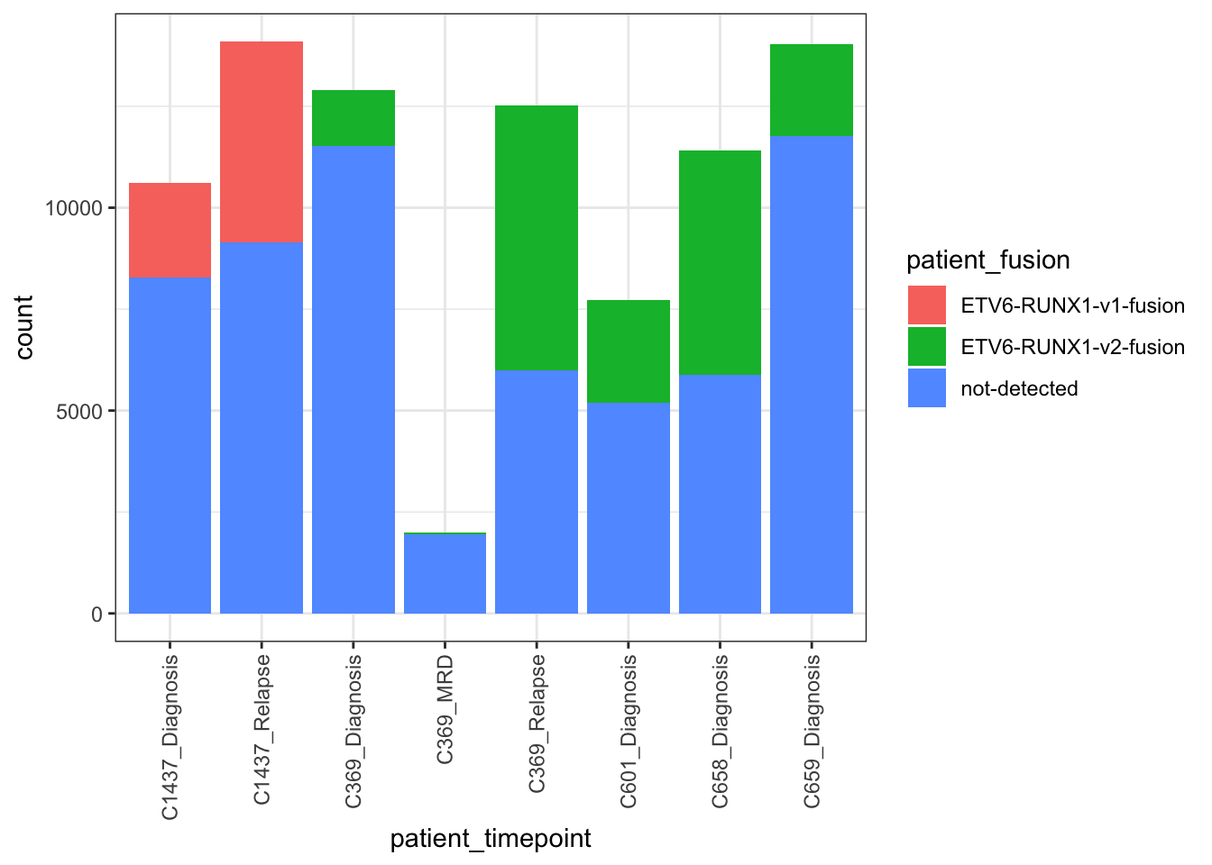
seu@meta.data %>%
  ggplot(aes(x = patient_timepoint,
             fill = patient_fusion)) +
  geom_bar(position = "fill") +  # key change to get proportions
  scale_y_continuous(labels = scales::percent) +  # optional: show % instead of 0–1
  theme_bw() +
  theme(axis.text.x = element_text(angle = 90, hjust = 1, vjust = 0.5)) +
  labs(y = "% cells with fusion detected")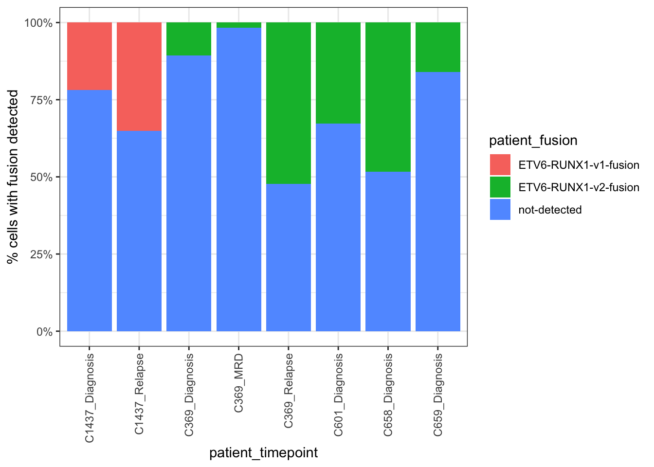
BoneMarrowMap reference
The BoneMarrowMap Symphony reference object and UMAP model are downloaded if not already present. These files are used to project query cells into the reference embedding.
projection_path = here("data/BoneMarrowMap")
# Set directory to store projection reference files
if(!dir.exists(projection_path)) dir.create(projection_path)

# Download Bone Marrow Reference - 344 Mb
rds <- paste0(projection_path, 'BoneMarrowMap_SymphonyReference.rds')
if(!file.exists(rds)){
  curl::curl_download('https://bonemarrowmap.s3.us-east-2.amazonaws.com/BoneMarrowMap_SymphonyReference.rds',
                      destfile = rds)
}

uwot <- paste0(projection_path, 'BoneMarrowMap_uwot_model.uwot')
if(!file.exists(uwot)){
  # Download uwot model file - 221 Mb
  curl::curl_download('https://bonemarrowmap.s3.us-east-2.amazonaws.com/BoneMarrowMap_uwot_model.uwot',
                      destfile = uwot)
}

# Load Symphony reference
ref <- readRDS(rds)
# Set uwot path for UMAP projection
ref$save_uwot_path <- uwot
Visualise BoneMarrowMap reference
A lightweight Seurat object is created from the Symphony reference for visualisation purposes. This object contains only UMAP coordinates and cell metadata (cell type labels, cycle phase, pseudotime), without gene expression counts.
ReferenceSeuratObj <- create_ReferenceObject(ref)

DimPlot(ReferenceSeuratObj, reduction = 'umap', group.by = 'CellType_Annotation_formatted',
        raster=FALSE, label=TRUE, label.size = 2) + NoLegend()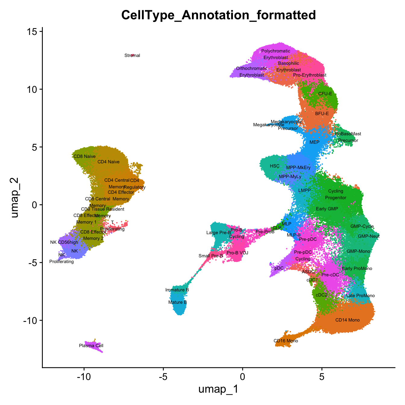
| Version | Author | Date |
|---|---|---|
| 1b5bb97 | Jovana Maksimovic | 2026-05-11 |
We can also visualize broader cell type labels which may simplify interpretation and downstream analysis.
DimPlot(ReferenceSeuratObj, reduction = 'umap', group.by = 'CellType_Broad',
        raster=FALSE, label=TRUE, label.size = 2) + NoLegend()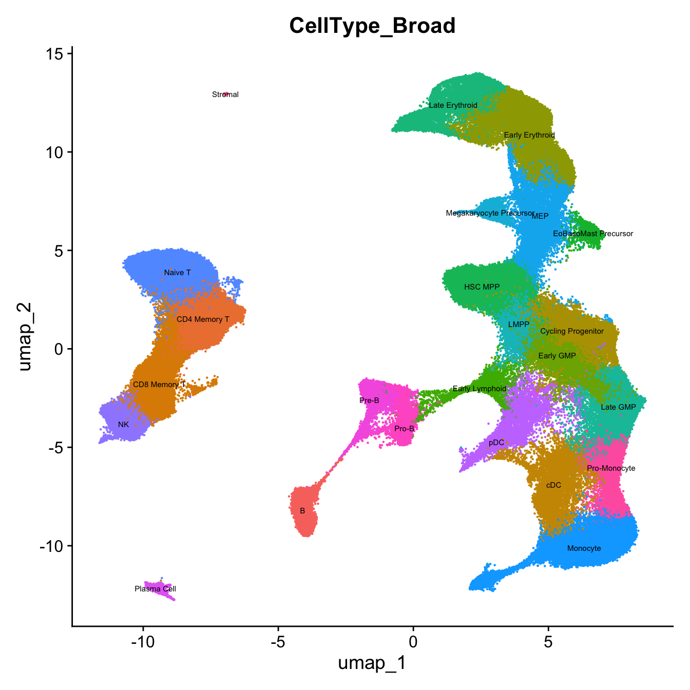
| Version | Author | Date |
|---|---|---|
| 1b5bb97 | Jovana Maksimovic | 2026-05-11 |
We can visualize other annotations too, including cell cycle phase and lineage pseudotime estimates.
p1 <- DimPlot(ReferenceSeuratObj, reduction = 'umap', group.by = 'CyclePhase', raster=FALSE)
p2 <- FeaturePlot(ReferenceSeuratObj, reduction = 'umap', features = 'Pseudotime', raster=FALSE)

p1 + p2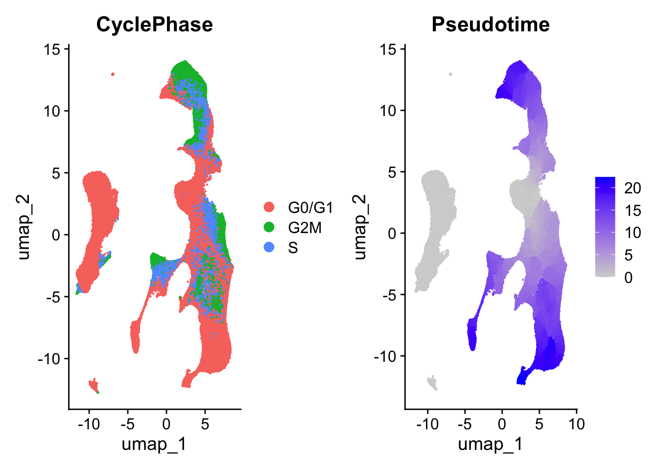
| Version | Author | Date |
|---|---|---|
| 1b5bb97 | Jovana Maksimovic | 2026-05-11 |
Project query onto the reference
Query cells are projected onto the BoneMarrowMap reference using Symphony, correcting for sample-level batch effects. Mapping error is then calculated per cell and used to flag low-quality projections. Cells with mapping error scores more than 3 MADs above the per-sample median are excluded from downstream analysis.
query <- seu
# batch variable to correct in the query data, set as NULL if no batches in query
batchvar <- 'Sample'

# Map query dataset using Symphony (Kang et al 2021)
query <- map_Query(
    exp_query = query@assays$RNA$counts,
    metadata_query = query@meta.data,
    ref_obj = ref,
    vars = batchvar
)
In leukaemia samples the mapping error distribution can vary broadly between samples, so outlier thresholds are applied per sample (3 MADs above the per-sample median).
# Run QC based on mapping error score, flag cells with mapping error >= 2.5 MADs above median
query <- query %>%
  calculate_MappingError(., reference = ref, MAD_threshold = 3,
                         threshold_by_donor = TRUE,
                         donor_key = batchvar) # threshold mapping error on a per-sample basis.

# Plot distribution by patient to ensure you are catching the tail
query@meta.data %>%
  ggplot(aes(x = mapping_error_score, fill = mapping_error_QC)) +
  geom_histogram(bins = 200) + facet_wrap(.~get(batchvar), ncol = 2)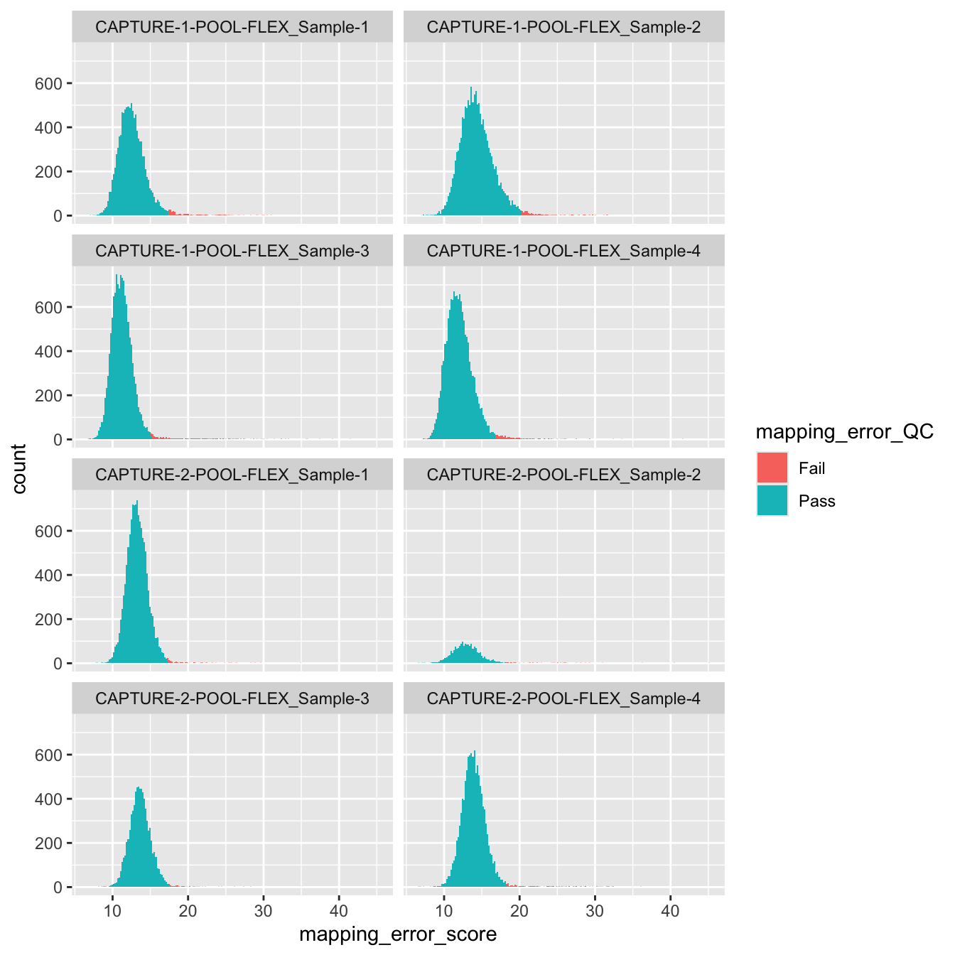
# Get QC Plots
QC_plots <- plot_MappingErrorQC(query)

# Plot together
patchwork::wrap_plots(QC_plots, ncol = 2)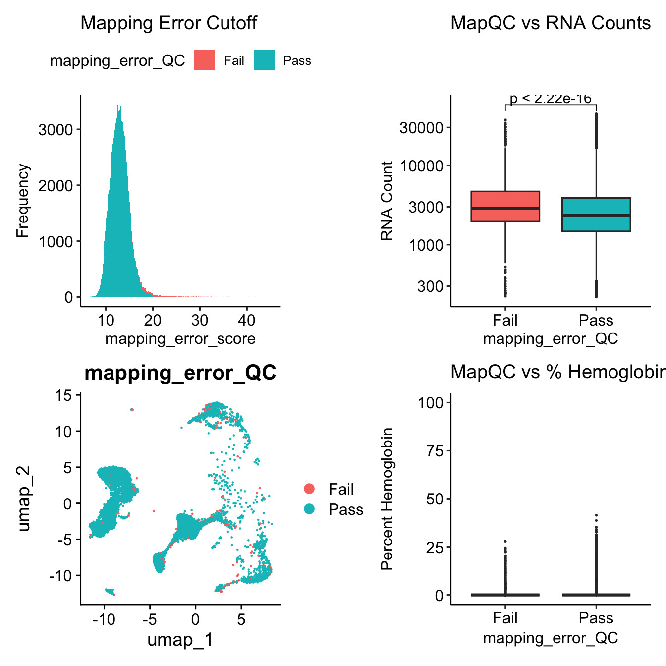
query@meta.data %>%
     dplyr::count(patient_timepoint, mapping_error_QC) %>%
     group_by(patient_timepoint) %>%
     mutate(pct = n / sum(n) * 100) %>%
     dplyr::filter(mapping_error_QC == "Fail") %>%
     ggplot(aes(x = reorder(patient_timepoint, pct), y = pct)) +
     geom_col(fill = "steelblue") +
     geom_text(aes(label = sprintf("%.1f%%", pct)), hjust = -0.1, size = 3) +
     coord_flip() +
     ylim(0, 4) +
     labs(x = NULL, y = "% cells failing BoneMarrowMap QC") +
     theme_minimal()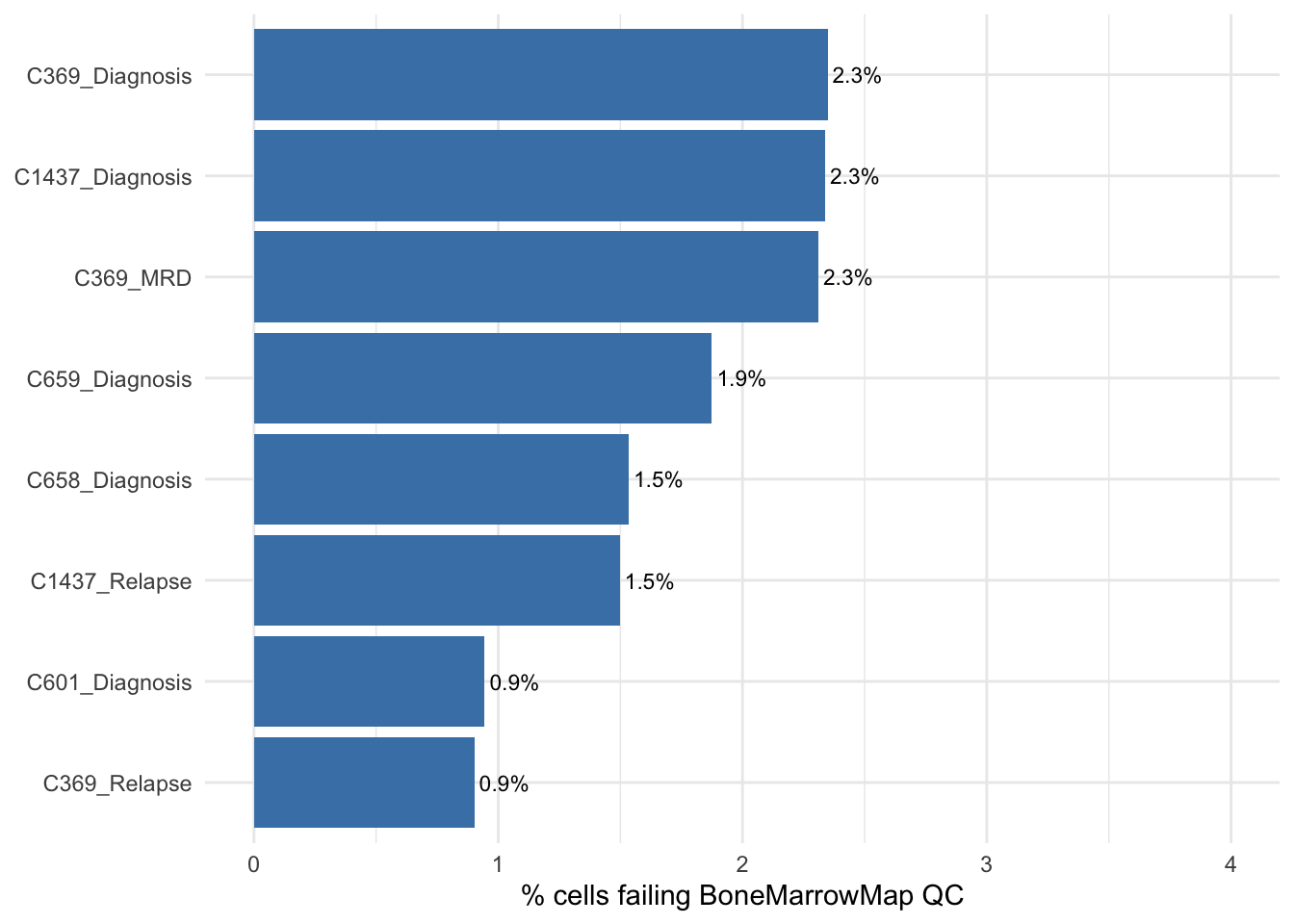
| Version | Author | Date |
|---|---|---|
| c4f8670 | Jovana Maksimovic | 2026-07-15 |
Cell type assignment
Cell identities are assigned by KNN classification using the 30
nearest neighbours in the reference embedding. Both precise
(predicted_CellType) and broad
(predicted_CellType_Broad) labels are transferred.
Fusion-positive cells are highlighted on the projected UMAP.
# Predict Hematopoietic Cell Types by KNN classification
query <- predict_CellTypes(
  query_obj = query,
  ref_obj = ref,
  initial_label = 'initial_CellType', # celltype assignments before filtering on mapping QC
  final_label = 'predicted_CellType'  # celltype assignments with map QC failing cells assigned as NA
)

DimPlot(query, reduction = 'umap_projected',
        group.by = c('predicted_CellType'),
        raster=FALSE, label=TRUE, label.size = 2) + NoLegend()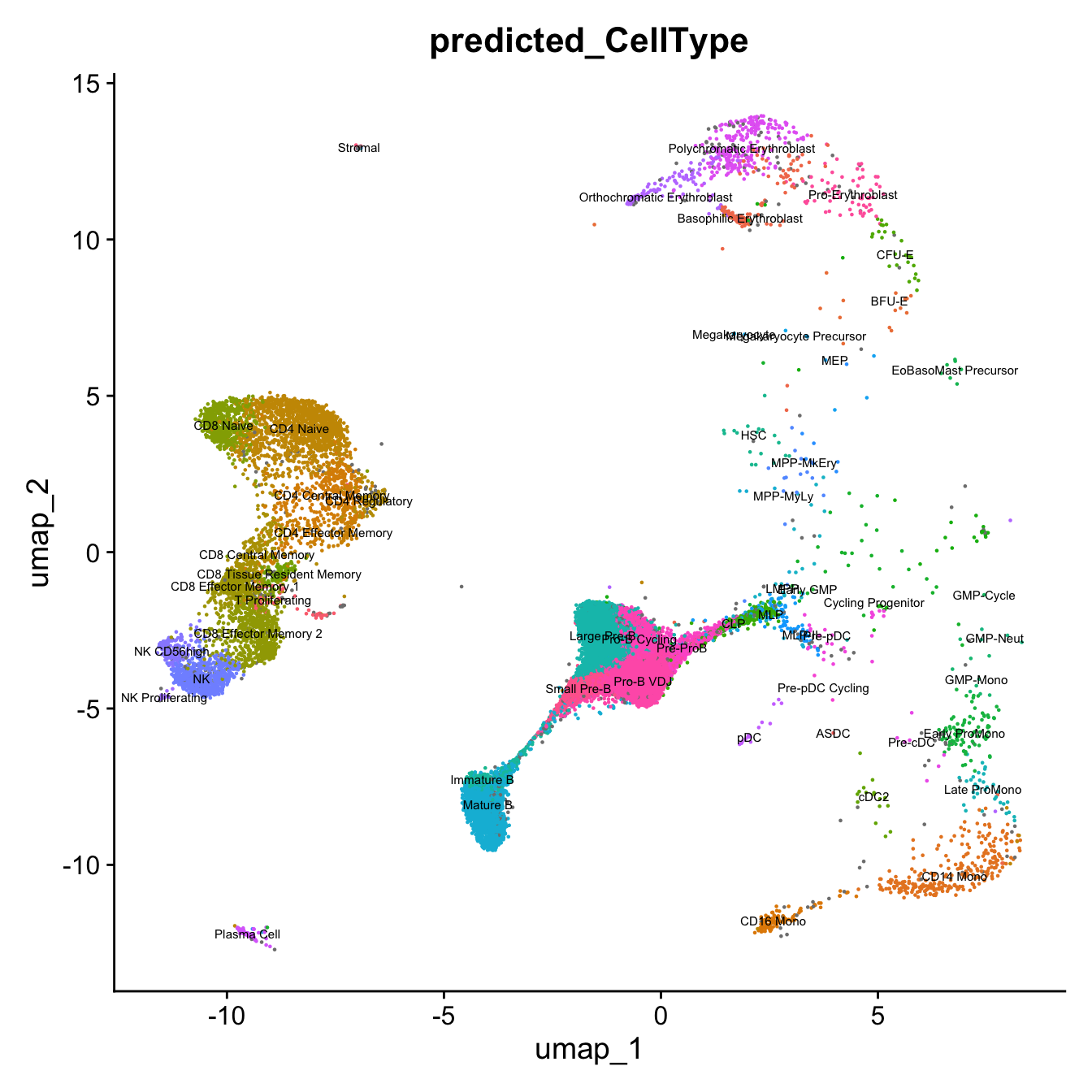
cells.highlight <- split(which(query$patient_fusion != "not-detected"),
                                query$patient_fusion[query$patient_fusion != "not-detected"])

DimPlot(query, reduction = 'umap_projected',
        group.by = c('predicted_CellType'),
        raster = FALSE,
        label = TRUE,
        label.size = 2.5,
        sizes.highlight = 0.1,
        repel = T,
        cells.highlight = cells.highlight,
        cols.highlight = setNames(c("red","purple"),
                                  names(cells.highlight))) +
  theme(legend.position = "bottom") -> p1

p1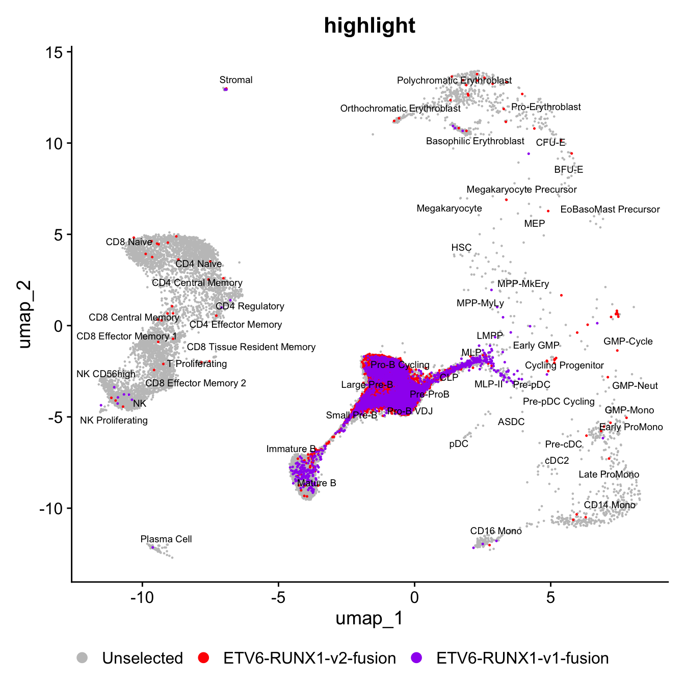
We can also visualize the broader cell type categories in case precise labels are too granular. These provide a simpler view of the data and can help guide cluster annotations if your dataset does not have many cells.
DimPlot(query, reduction = 'umap_projected',
        group.by = c('predicted_CellType_Broad'),
        raster = FALSE, label=TRUE, label.size = 2.5) +
  paletteer::scale_color_paletteer_d(palette = "ggsci::default_ucscgb") + NoLegend()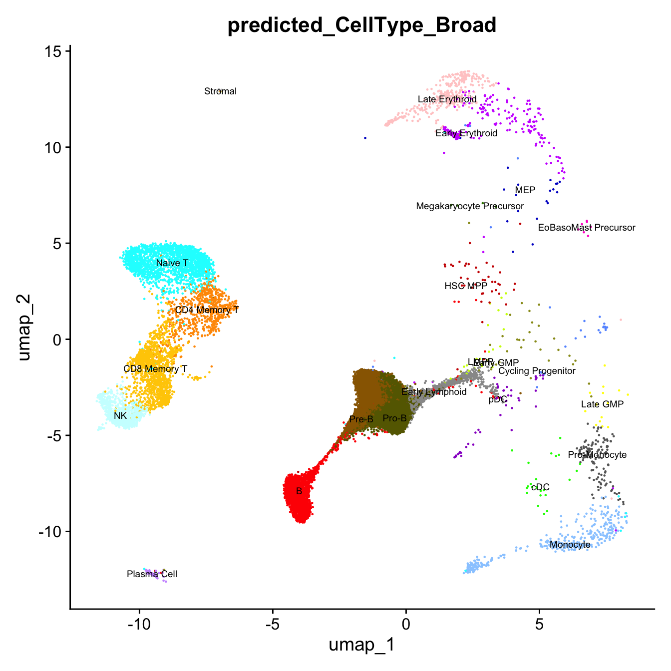
# Cache the BoneMarrowMap projection result (map_Query + predict_CellTypes).
# Loading this avoids re-running the Symphony projection on subsequent rebuilds.
out_proj <- here("data", "RDS", "ball_exp2_projected.seu.rds")
if(!file.exists(out_proj)) saveRDS(query, out_proj)
cells.highlight <- split(which(query$patient_fusion != "not-detected"),
query$patient_fusion[query$patient_fusion != "not-detected"])
DimPlot(query, reduction = 'umap_projected',
group.by = c('predicted_CellType_Broad'),
split.by = "patient_timepoint",
raster = FALSE,
label = TRUE,
label.size = 2.5,
sizes.highlight = 0.1,
repel = T,
ncol = 2,
cells.highlight = cells.highlight,
cols.highlight = setNames(c("red","purple"),
names(cells.highlight))) +
theme(legend.position = "bottom") -> p1
p1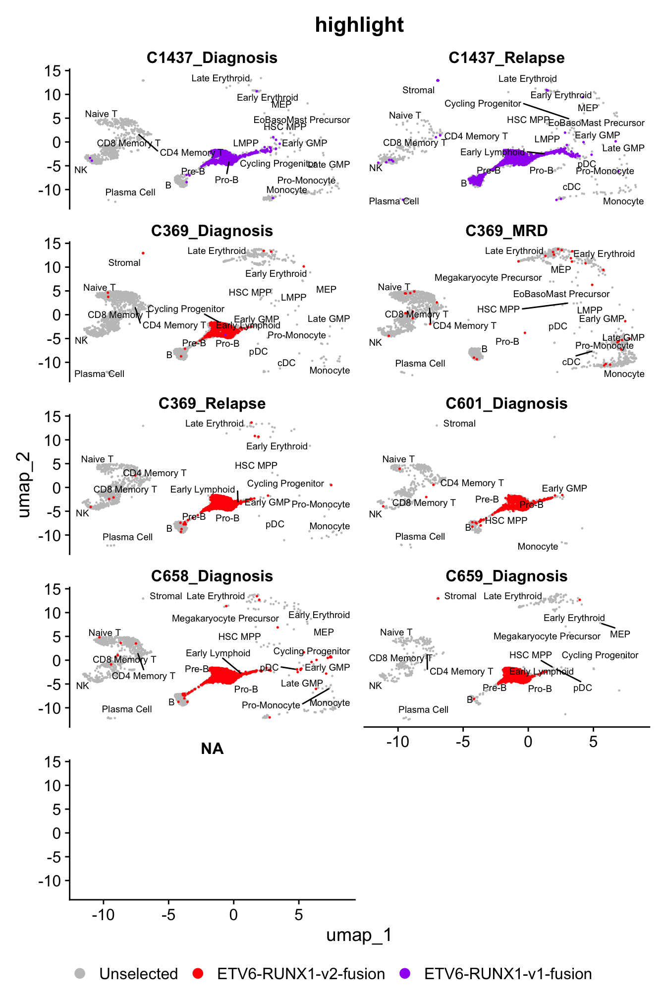
Pseudotime and projection density
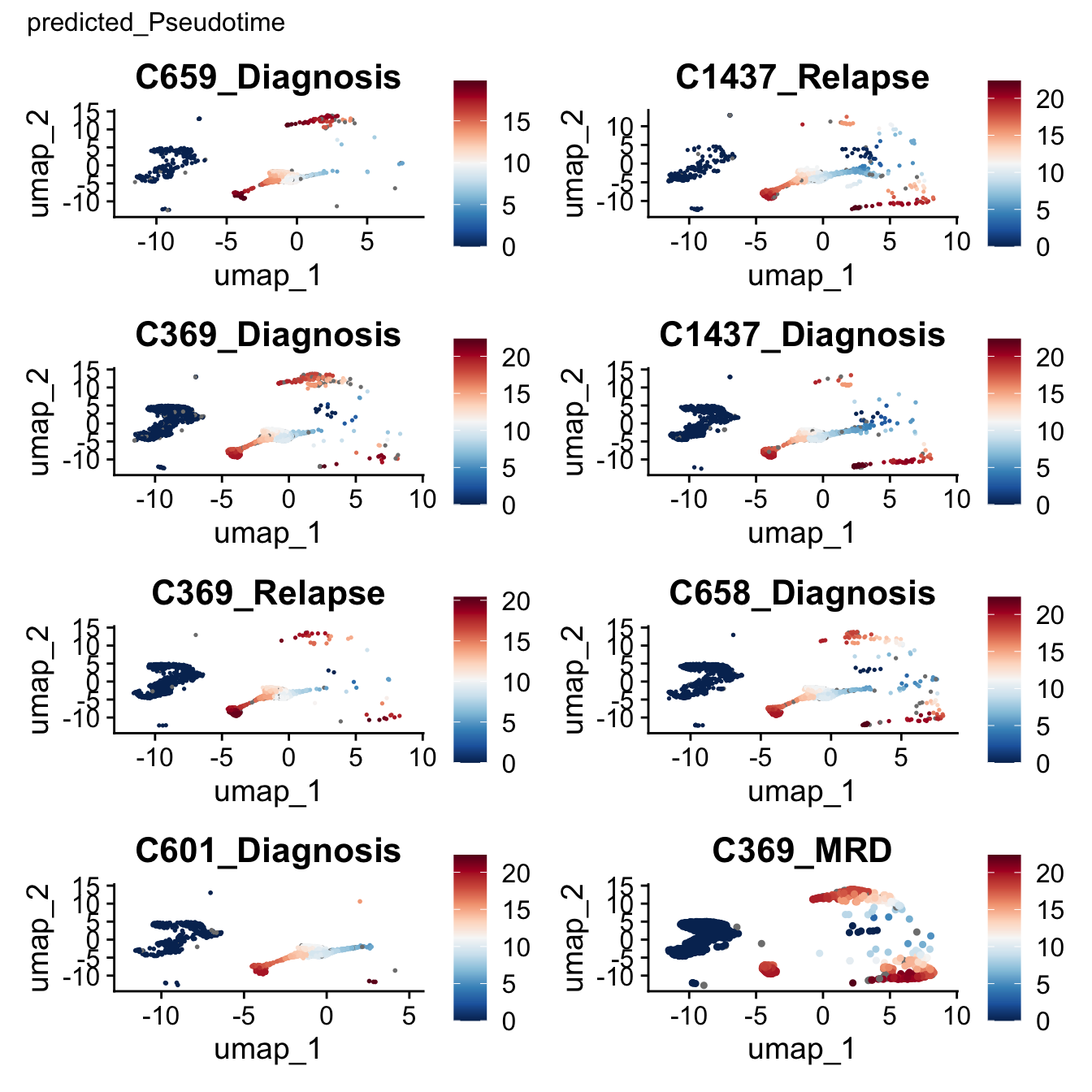
Each query cell is assigned a hematopoietic pseudotime score based on its 30 nearest neighbours in the reference UMAP. Per-sample pseudotime distributions are visualised to assess the developmental stage of cells across patients and timepoints.
# Predict Pseudotime values by KNN
query <- predict_Pseudotime(
  query_obj = query,
  ref_obj = ref,
  initial_label = 'initial_Pseudotime',  # pseudotime assignments before filtering on mapping QC
  final_label = 'predicted_Pseudotime'   # pseudotime assignments with map QC failing cells assigned as NA
)

# Visualize Hematopoietic Pseudotime in query data
lapply(unique(query$patient_timepoint), function(samp){
  FeaturePlot(subset(query, query$patient_timepoint == samp),
            features = c('predicted_Pseudotime')) +
    ggtitle(samp) &
  scale_color_gradientn(colors = rev(RColorBrewer::brewer.pal(11, 'RdBu')))
}) -> p

wrap_plots(p, ncol = 2) +
  plot_annotation(
    title = "predicted_Pseudotime",
    theme = theme(
      plot.title  = element_text(size = 12),
      axis.text   = element_text(size = 8),
      legend.text = element_text(size = 8),
      axis.title  = element_text(size = 10)
    )
  )
Projection density
The density of query cells across the hematopoietic hierarchy is visualised per sample against a down-sampled reference background, showing where each patient’s cells sit within the normal bone marrow landscape.
# Set batch/condition to be visualized individually
batch_key <- 'patient_timepoint'

# returns a list of plots for each donor from a pre-specified batch variable
projection_plots <- plot_Projection_byDonor(
  query_obj = query,
  batch_key = batch_key,
  ref_obj = ref,
  Hierarchy_only = FALSE, # Whether to exclude T/NK/Plasma/Stromal cells
  downsample_reference = TRUE,
  downsample_frac = 0.25,   # down-sample reference cells to 25%; reduces figure file size
  query_point_size = 0.2,   # adjust size of query cells based on # of cells
  saveplot = TRUE,
  save_folder = 'projectionFigures/'
)

# show plots together with patchwork.
patchwork::wrap_plots(projection_plots, ncol = 2)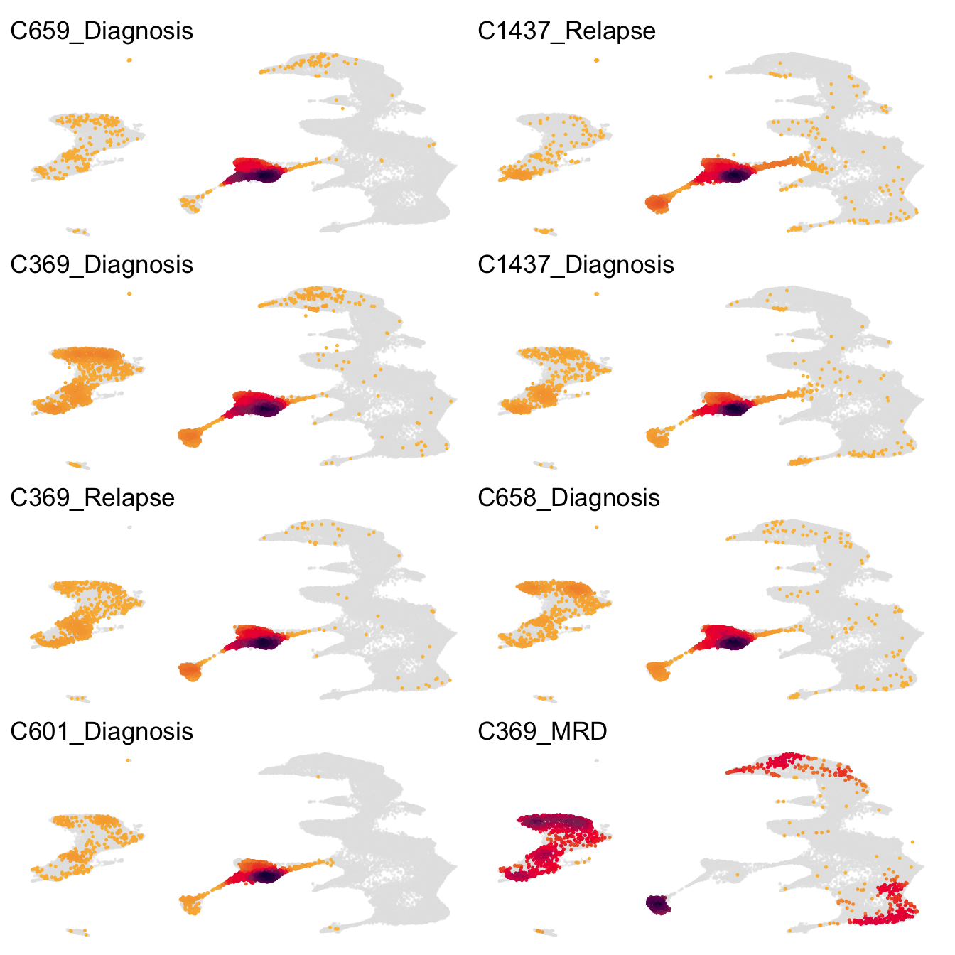
Cell type composition per sample
Cell type composition is summarised per sample, restricted to cells with KNN classification probability >0.5 (i.e. >50% of nearest neighbours from the reference agree on the assigned label). Results are presented as proportions in both long and wide format, and visualised as a heatmap.
query_composition <- get_Composition(
  query_obj = query,
  donor_key = 'patient_timepoint',
  celltype_label = 'predicted_CellType',
  mapQC_col = 'mapping_error_QC',
  knn_prob_cutoff = 0.5,
  return_type = 'long')

query_composition
# A tibble: 293 × 4
patient_timepoint predicted_CellType count proportion
<fct> <chr> <int> <dbl>
1 C1437_Diagnosis Pro-B VDJ 7325 0.748
2 C1437_Diagnosis Small Pre-B 680 0.0695
3 C1437_Diagnosis Large Pre-B 388 0.0396
4 C1437_Diagnosis Pro-B Cycling 353 0.0361
5 C1437_Diagnosis Mature B 140 0.0143
6 C1437_Diagnosis CD8 Effector Memory 2 136 0.0139
7 C1437_Diagnosis NK 126 0.0129
8 C1437_Diagnosis CD4 Naive 113 0.0115
9 C1437_Diagnosis Pre-ProB 90 0.00919
10 C1437_Diagnosis CD16 Mono 63 0.00644
# ℹ 283 more rowsquery_composition %>%
dplyr::filter(proportion > 0.01) %>%
mutate(predicted_CellType = fct_drop(predicted_CellType)) %>%
ggplot(aes(x = patient_timepoint, y = proportion, fill= predicted_CellType)) +
geom_bar(stat = "identity", outline = 1) +
paletteer::scale_fill_paletteer_d(palette = "pals::glasbey") +
guides(fill = guide_legend(ncol = 3)) +
theme(legend.position = "bottom",
axis.text = element_text(angle = 90, hjust = 1, vjust = 0.5))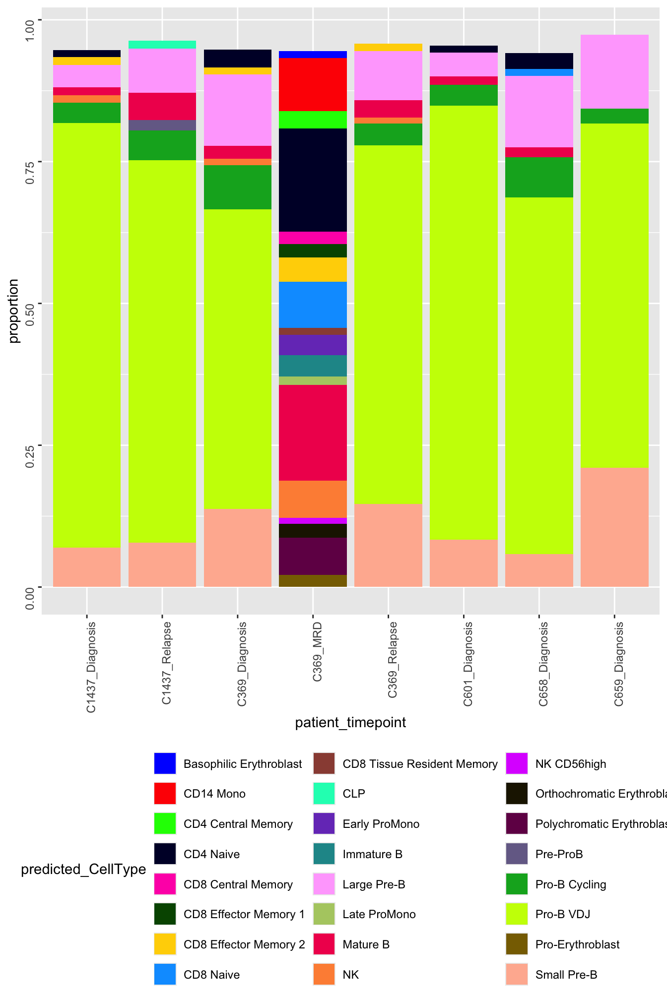
The inverse view — how much each sample contributes to each broad cell type — reveals whether any cell type is dominated by a single donor.
# get_Composition only supports fine-grained labels (no knn_prob col for Broad);
# compute directly from metadata instead, using the same mapping_error_QC filter
query@meta.data %>%
  filter(mapping_error_QC == "Pass") %>%
  dplyr::count(patient_timepoint, predicted_CellType_Broad) %>%
  group_by(predicted_CellType_Broad) %>%
  mutate(prop = n / sum(n),
         total_cells = sum(n)) %>%
  ungroup() %>%
  filter(total_cells >= 10) %>%
  mutate(predicted_CellType_Broad = fct_reorder(predicted_CellType_Broad, total_cells, .desc = TRUE)) %>%
  ggplot(aes(x = predicted_CellType_Broad, y = prop, fill = patient_timepoint)) +
  geom_bar(stat = "identity") +
  paletteer::scale_fill_paletteer_d(palette = "pals::glasbey") +
  scale_y_continuous(expand = expansion(mult = c(0, 0.05)),
                     labels = scales::percent) +
  labs(x = NULL, y = "Proportion of cells", fill = "Sample") +
  guides(fill = guide_legend(ncol = 2)) +
  theme(axis.text.x = element_text(angle = 45, hjust = 1),
        legend.position = "bottom")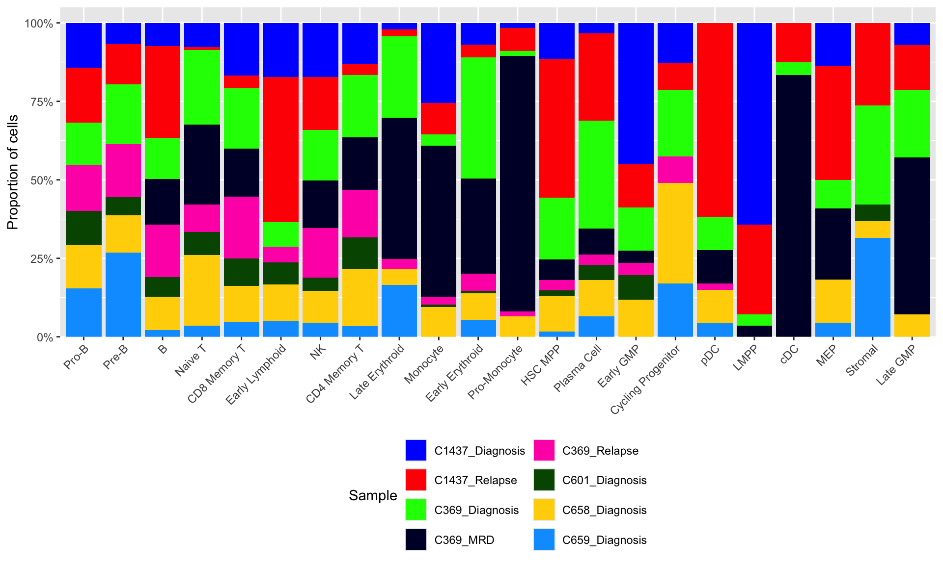
| Version | Author | Date |
|---|---|---|
| c4f8670 | Jovana Maksimovic | 2026-07-15 |
Wide format with cell counts.
query_composition_wide_counts <- get_Composition(
  query_obj = query,
  donor_key = 'patient_timepoint',
  celltype_label = 'predicted_CellType',
  mapQC_col = 'mapping_error_QC',
  knn_prob_cutoff = 0.5,
  return_type = 'count')

query_composition_wide_counts
# A tibble: 8 × 55
patient_timepoint `Pro-B VDJ` `Small Pre-B` `Large Pre-B` `Pro-B Cycling`
<fct> <int> <int> <int> <int>
1 C1437_Diagnosis 7325 680 388 353
2 C1437_Relapse 8683 1008 1009 684
3 C369_Diagnosis 6091 1594 1460 906
4 C369_MRD 1 0 0 0
5 C369_Relapse 7443 1722 1016 454
6 C601_Diagnosis 5578 611 309 266
7 C658_Diagnosis 6727 623 1346 757
8 C659_Diagnosis 7865 2725 1686 341
# ℹ 50 more variables: `Mature B` <int>, `CD8 Effector Memory 2` <int>,
# NK <int>, `CD4 Naive` <int>, `Pre-ProB` <int>, `CD16 Mono` <int>,
# `CD8 Effector Memory 1` <int>, CLP <int>, `CD4 Central Memory` <int>,
# `Immature B` <int>, `CD8 Naive` <int>, `CD14 Mono` <int>,
# `NK CD56high` <int>, `CD4 Effector Memory` <int>, `T Proliferating` <int>,
# `CD4 Regulatory` <int>, `CD8 Central Memory` <int>,
# `CD8 Tissue Resident Memory` <int>, MLP <int>, LMPP <int>, …Wide format with proportions.
query_composition_wide_props <- get_Composition(
  query_obj = query,
  donor_key = 'patient_timepoint',
  celltype_label = 'predicted_CellType',
  mapQC_col = 'mapping_error_QC',
  knn_prob_cutoff = 0.5,
  return_type = 'proportion')

query_composition_wide_props
# A tibble: 8 × 55
patient_timepoint `Pro-B VDJ` `Small Pre-B` `Large Pre-B` `Pro-B Cycling`
<fct> <dbl> <dbl> <dbl> <dbl>
1 C1437_Diagnosis 0.748 0.0695 0.0396 0.0361
2 C1437_Relapse 0.674 0.0782 0.0783 0.0531
3 C369_Diagnosis 0.527 0.138 0.126 0.0785
4 C369_MRD 0.000553 0 0 0
5 C369_Relapse 0.632 0.146 0.0863 0.0386
6 C601_Diagnosis 0.765 0.0838 0.0424 0.0365
7 C658_Diagnosis 0.629 0.0582 0.126 0.0707
8 C659_Diagnosis 0.607 0.210 0.130 0.0263
# ℹ 50 more variables: `Mature B` <dbl>, `CD8 Effector Memory 2` <dbl>,
# NK <dbl>, `CD4 Naive` <dbl>, `Pre-ProB` <dbl>, `CD16 Mono` <dbl>,
# `CD8 Effector Memory 1` <dbl>, CLP <dbl>, `CD4 Central Memory` <dbl>,
# `Immature B` <dbl>, `CD8 Naive` <dbl>, `CD14 Mono` <dbl>,
# `NK CD56high` <dbl>, `CD4 Effector Memory` <dbl>, `T Proliferating` <dbl>,
# `CD4 Regulatory` <dbl>, `CD8 Central Memory` <dbl>,
# `CD8 Tissue Resident Memory` <dbl>, MLP <dbl>, LMPP <dbl>, …Heatmap of cell type composition by sample.
# Simple heatmap to visualize composition of projected samples
p <- query_composition_wide_props %>%
  # show celltypes present in >1% of total cells
  select(patient_timepoint,
         colnames(query_composition_wide_props)[-1][colSums(query_composition_wide_props[-1]) > 0.01]) %>%
  # convert to matrix and display heatmap
  column_to_rownames('patient_timepoint') %>% data.matrix() %>% ComplexHeatmap::Heatmap()
p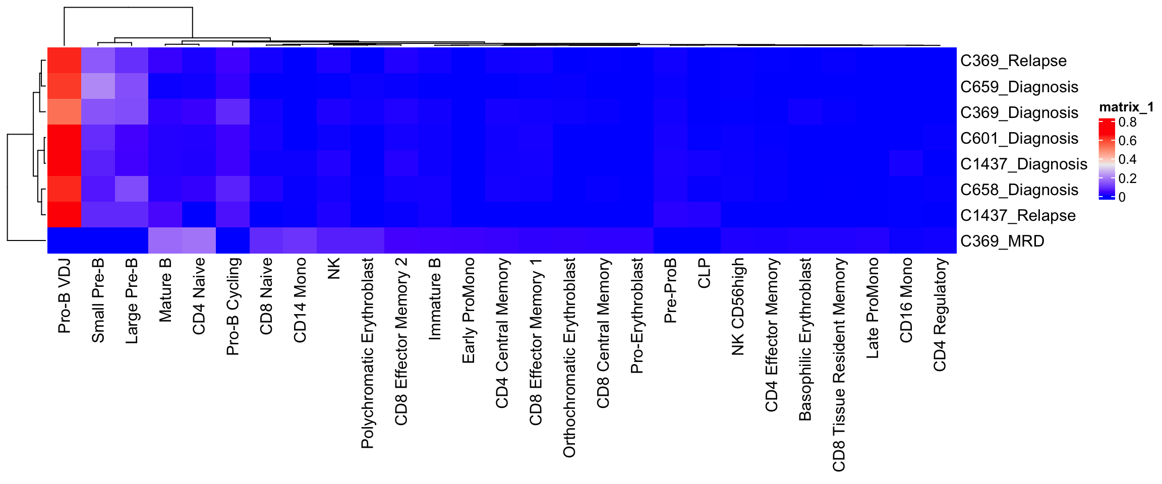
Save outputs
out <- here("data", "RDS", "ball_exp2_annotated.seu.rds")
if(!file.exists(out)) saveRDS(query, out)
fs::file_chmod(out, "664")
try(fs::file_chown(out, group_id = "oshlack_lab"),
    silent = TRUE)
Session info
sessioninfo::session_info()─ Session info ───────────────────────────────────────────────────────────────
setting value
version R version 4.4.1 (2024-06-14)
os macOS 15.7.9
system aarch64, darwin20
ui X11
language (EN)
collate en_US.UTF-8
ctype en_US.UTF-8
tz Australia/Melbourne
date 2026-08-25
pandoc 3.8.3 @ /Applications/RStudio.app/Contents/Resources/app/quarto/bin/tools/aarch64/ (via rmarkdown)
quarto 1.9.38 @ /Applications/RStudio.app/Contents/Resources/app/quarto/bin/quarto
─ Packages ───────────────────────────────────────────────────────────────────
! package * version date (UTC) lib source
P abind 1.4-8 2024-09-12 [?] CRAN (R 4.4.1)
P annotate 1.84.0 2024-11-08 [?] Bioconduc~
P AnnotationDbi 1.68.0 2024-11-08 [?] Bioconduc~
AUCell 1.28.0 2024-11-08 [1] Bioconductor 3.20 (R 4.4.1)
P backports 1.5.0 2024-05-23 [?] CRAN (R 4.4.1)
P Biobase * 2.66.0 2024-11-08 [?] Bioconduc~
P BiocGenerics * 0.52.0 2024-11-08 [?] Bioconduc~
P BiocManager 1.30.27 2025-11-14 [?] CRAN (R 4.4.3)
P BiocNeighbors 2.0.1 2024-11-28 [?] Bioconduc~
P Biostrings 2.74.1 2024-12-16 [?] Bioconduc~
P bit 4.6.0 2025-03-06 [?] CRAN (R 4.4.1)
P bit64 4.6.0-1 2025-01-16 [?] CRAN (R 4.4.1)
P blob 1.2.4 2023-03-17 [?] CRAN (R 4.4.0)
BoneMarrowMap * 0.1.0 2025-06-04 [1] Github (andygxzeng/BoneMarrowMap@81f2756)
P broom 1.0.8 2025-03-28 [?] CRAN (R 4.4.1)
P bslib 0.9.0 2025-01-30 [?] CRAN (R 4.4.1)
P cachem 1.1.0 2024-05-16 [?] CRAN (R 4.4.1)
P Cairo 1.6-2 2023-11-28 [?] CRAN (R 4.4.1)
P callr 3.7.6 2024-03-25 [?] CRAN (R 4.4.0)
P car 3.1-3 2024-09-27 [?] CRAN (R 4.4.1)
P carData 3.0-5 2022-01-06 [?] CRAN (R 4.4.1)
P circlize 0.4.16 2024-02-20 [?] CRAN (R 4.4.0)
P cli 3.6.5 2025-04-23 [?] CRAN (R 4.4.1)
P clue 0.3-66 2024-11-13 [?] CRAN (R 4.4.1)
P cluster 2.1.6 2023-12-01 [?] CRAN (R 4.4.1)
P codetools 0.2-20 2024-03-31 [?] CRAN (R 4.4.1)
P colorspace 2.1-1 2024-07-26 [?] CRAN (R 4.4.1)
P ComplexHeatmap 2.22.0 2024-11-08 [?] Bioconduc~
P cowplot 1.1.3 2024-01-22 [?] CRAN (R 4.4.0)
P crayon 1.5.3 2024-06-20 [?] CRAN (R 4.4.1)
P data.table 1.18.2.1 2026-01-27 [?] CRAN (R 4.4.3)
P DBI 1.2.3 2024-06-02 [?] CRAN (R 4.4.1)
P DelayedArray 0.32.0 2024-11-08 [?] Bioconduc~
P DelayedMatrixStats 1.28.1 2025-01-09 [?] Bioconduc~
P deldir 2.0-4 2024-02-28 [?] CRAN (R 4.4.1)
P digest 0.6.37 2024-08-19 [?] CRAN (R 4.4.1)
P doParallel 1.0.17 2022-02-07 [?] CRAN (R 4.4.0)
P dotCall64 1.2 2024-10-04 [?] CRAN (R 4.4.1)
P dplyr * 1.1.4 2023-11-17 [?] CRAN (R 4.4.0)
P evaluate 1.0.3 2025-01-10 [?] CRAN (R 4.4.1)
P farver 2.1.2 2024-05-13 [?] CRAN (R 4.4.1)
P fastDummies 1.7.5 2025-01-20 [?] CRAN (R 4.4.1)
P fastmap 1.2.0 2024-05-15 [?] CRAN (R 4.4.1)
P fitdistrplus 1.2-2 2025-01-07 [?] CRAN (R 4.4.1)
P forcats * 1.0.0 2023-01-29 [?] CRAN (R 4.4.0)
P foreach 1.5.2 2022-02-02 [?] CRAN (R 4.4.0)
P Formula 1.2-5 2023-02-24 [?] CRAN (R 4.4.1)
P fs 1.6.6 2025-04-12 [?] CRAN (R 4.4.1)
P future 1.49.0 2025-05-09 [?] CRAN (R 4.4.1)
P future.apply 1.11.3 2024-10-27 [?] CRAN (R 4.4.1)
P generics 0.1.4 2025-05-09 [?] CRAN (R 4.4.1)
P GenomeInfoDb * 1.42.3 2025-01-27 [?] Bioconduc~
P GenomeInfoDbData 1.2.13 2025-05-28 [?] Bioconductor
P GenomicRanges * 1.58.0 2024-11-08 [?] Bioconduc~
P GetoptLong 1.0.5 2020-12-15 [?] CRAN (R 4.4.1)
P getPass 0.2-4 2023-12-10 [?] CRAN (R 4.4.1)
P ggplot2 * 4.0.2 2026-02-03 [?] CRAN (R 4.4.3)
ggpointdensity 0.2.0 2025-05-16 [1] CRAN (R 4.4.1)
P ggpubr 0.6.0 2023-02-10 [?] CRAN (R 4.4.0)
P ggrepel 0.9.6 2024-09-07 [?] CRAN (R 4.4.1)
P ggridges 0.5.6 2024-01-23 [?] CRAN (R 4.4.0)
P ggsignif 0.6.4 2022-10-13 [?] CRAN (R 4.4.0)
P git2r 0.36.2 2025-03-29 [?] CRAN (R 4.4.1)
P GlobalOptions 0.1.2 2020-06-10 [?] CRAN (R 4.4.1)
P globals 0.18.0 2025-05-08 [?] CRAN (R 4.4.1)
P glue * 1.8.0 2024-09-30 [?] CRAN (R 4.4.1)
P goftest 1.2-3 2021-10-07 [?] CRAN (R 4.4.1)
graph 1.84.1 2025-01-02 [1] Bioconductor 3.20 (R 4.4.2)
P gridExtra 2.3 2017-09-09 [?] CRAN (R 4.4.1)
GSEABase 1.68.0 2024-11-08 [1] Bioconductor 3.20 (R 4.4.1)
P gtable 0.3.6 2024-10-25 [?] CRAN (R 4.4.1)
P harmony 1.2.3 2024-11-27 [?] CRAN (R 4.4.1)
P here * 1.0.1 2020-12-13 [?] CRAN (R 4.4.1)
P hms 1.1.3 2023-03-21 [?] CRAN (R 4.4.0)
P htmltools 0.5.8.1 2024-04-04 [?] CRAN (R 4.4.1)
P htmlwidgets 1.6.4 2023-12-06 [?] CRAN (R 4.4.0)
P httpuv 1.6.16 2025-04-16 [?] CRAN (R 4.4.1)
P httr 1.4.7 2023-08-15 [?] CRAN (R 4.4.0)
P ica 1.0-3 2022-07-08 [?] CRAN (R 4.4.1)
P igraph 2.1.4 2025-01-23 [?] CRAN (R 4.4.1)
P IRanges * 2.40.1 2024-12-05 [?] Bioconduc~
P irlba 2.3.5.1 2022-10-03 [?] CRAN (R 4.4.0)
P iterators 1.0.14 2022-02-05 [?] CRAN (R 4.4.1)
jcolors 0.0.5 2025-06-04 [1] Github (jaredhuling/jcolors@7c29a50)
P jquerylib 0.1.4 2021-04-26 [?] CRAN (R 4.4.0)
P jsonlite 2.0.0 2025-03-27 [?] CRAN (R 4.4.1)
P KEGGREST 1.46.0 2024-11-08 [?] Bioconduc~
P KernSmooth 2.23-24 2024-05-17 [?] CRAN (R 4.4.1)
P knitr 1.50 2025-03-16 [?] CRAN (R 4.4.1)
P labeling 0.4.3 2023-08-29 [?] CRAN (R 4.4.1)
P later 1.4.2 2025-04-08 [?] CRAN (R 4.4.1)
P lattice 0.22-6 2024-03-20 [?] CRAN (R 4.4.1)
P lazyeval 0.2.2 2019-03-15 [?] CRAN (R 4.4.1)
P lifecycle 1.0.4 2023-11-07 [?] CRAN (R 4.4.1)
P listenv 0.9.1 2024-01-29 [?] CRAN (R 4.4.1)
P lmtest 0.9-40 2022-03-21 [?] CRAN (R 4.4.1)
P lubridate * 1.9.4 2024-12-08 [?] CRAN (R 4.4.1)
P magrittr 2.0.3 2022-03-30 [?] CRAN (R 4.4.1)
P MASS 7.3-60.2 2024-04-26 [?] CRAN (R 4.4.1)
P Matrix 1.7-0 2024-04-26 [?] CRAN (R 4.4.1)
P MatrixGenerics * 1.18.1 2025-01-09 [?] Bioconduc~
P matrixStats * 1.5.0 2025-01-07 [?] CRAN (R 4.4.1)
P memoise 2.0.1 2021-11-26 [?] CRAN (R 4.4.0)
P mime 0.13 2025-03-17 [?] CRAN (R 4.4.1)
P miniUI 0.1.2 2025-04-17 [?] CRAN (R 4.4.1)
P nlme 3.1-164 2023-11-27 [?] CRAN (R 4.4.1)
P paletteer 1.6.0 2024-01-21 [?] CRAN (R 4.4.0)
P parallelly 1.45.0 2025-06-02 [?] CRAN (R 4.4.1)
P patchwork * 1.3.0 2024-09-16 [?] CRAN (R 4.4.1)
P pbapply 1.7-4 2025-07-20 [?] CRAN (R 4.4.1)
P pillar 1.10.2 2025-04-05 [?] CRAN (R 4.4.1)
P pkgconfig 2.0.3 2019-09-22 [?] CRAN (R 4.4.1)
P plotly 4.10.4 2024-01-13 [?] CRAN (R 4.4.0)
P plyr 1.8.9 2023-10-02 [?] CRAN (R 4.4.1)
P png 0.1-8 2022-11-29 [?] CRAN (R 4.4.1)
P polyclip 1.10-7 2024-07-23 [?] CRAN (R 4.4.1)
P prismatic 1.1.2 2024-04-10 [?] CRAN (R 4.4.1)
P processx 3.8.6 2025-02-21 [?] CRAN (R 4.4.1)
P progressr 0.15.1 2024-11-22 [?] CRAN (R 4.4.1)
P promises 1.3.3 2025-05-29 [?] CRAN (R 4.4.1)
P ps 1.9.1 2025-04-12 [?] CRAN (R 4.4.1)
P purrr * 1.0.4 2025-02-05 [?] CRAN (R 4.4.1)
P R.methodsS3 1.8.2 2022-06-13 [?] CRAN (R 4.4.1)
P R.oo 1.27.1 2025-05-02 [?] CRAN (R 4.4.1)
P R.utils 2.13.0 2025-02-24 [?] CRAN (R 4.4.1)
P R6 2.6.1 2025-02-15 [?] CRAN (R 4.4.1)
P ragg 1.4.0 2025-04-10 [?] CRAN (R 4.4.1)
P RANN 2.6.2 2024-08-25 [?] CRAN (R 4.4.1)
P RColorBrewer 1.1-3 2022-04-03 [?] CRAN (R 4.4.1)
P Rcpp 1.1.1-1.1 2026-04-24 [?] CRAN (R 4.4.1)
P RcppAnnoy 0.0.22 2024-01-23 [?] CRAN (R 4.4.1)
P RcppHNSW 0.6.0 2024-02-04 [?] CRAN (R 4.4.1)
P readr * 2.1.5 2024-01-10 [?] CRAN (R 4.4.0)
P rematch2 2.1.2 2020-05-01 [?] CRAN (R 4.4.0)
renv 1.1.4 2025-03-20 [1] CRAN (R 4.4.1)
P reshape2 1.4.4 2020-04-09 [?] CRAN (R 4.4.0)
P reticulate 1.42.0 2025-03-25 [?] CRAN (R 4.4.1)
P rjson 0.2.23 2024-09-16 [?] CRAN (R 4.4.1)
P rlang 1.1.6 2025-04-11 [?] CRAN (R 4.4.1)
P rmarkdown 2.29 2024-11-04 [?] CRAN (R 4.4.1)
P ROCR 1.0-11 2020-05-02 [?] CRAN (R 4.4.0)
P rprojroot 2.0.4 2023-11-05 [?] CRAN (R 4.4.1)
P RSpectra 0.16-2 2024-07-18 [?] CRAN (R 4.4.0)
P RSQLite 2.4.0 2025-05-31 [?] CRAN (R 4.4.1)
P rstatix 0.7.2 2023-02-01 [?] CRAN (R 4.4.0)
P rstudioapi 0.17.1 2024-10-22 [?] CRAN (R 4.4.1)
P Rtsne 0.17 2023-12-07 [?] CRAN (R 4.4.1)
P S4Arrays 1.6.0 2024-11-08 [?] Bioconduc~
P S4Vectors * 0.44.0 2024-11-08 [?] Bioconduc~
P S7 0.2.0 2024-11-07 [?] CRAN (R 4.4.1)
P sass 0.4.10 2025-04-11 [?] CRAN (R 4.4.1)
P scales * 1.4.0 2025-04-24 [?] CRAN (R 4.4.1)
P scattermore 1.2 2023-06-12 [?] CRAN (R 4.4.0)
P sctransform 0.4.2 2025-04-30 [?] CRAN (R 4.4.1)
P sessioninfo 1.2.3 2025-02-05 [?] CRAN (R 4.4.1)
P Seurat * 5.3.0 2025-04-23 [?] CRAN (R 4.4.1)
P SeuratObject * 5.1.0 2025-04-22 [?] CRAN (R 4.4.1)
P shape 1.4.6.1 2024-02-23 [?] CRAN (R 4.4.1)
P shiny 1.10.0 2024-12-14 [?] CRAN (R 4.4.1)
P SingleCellExperiment * 1.28.1 2024-11-23 [?] Bioconduc~
P sp * 2.2-0 2025-02-01 [?] CRAN (R 4.4.1)
P spam 2.11-1 2025-01-20 [?] CRAN (R 4.4.1)
P SparseArray 1.6.2 2025-02-20 [?] Bioconduc~
P sparseMatrixStats 1.18.0 2024-11-08 [?] Bioconduc~
P spatstat.data 3.1-6 2025-03-17 [?] CRAN (R 4.4.1)
P spatstat.explore 3.4-3 2025-05-21 [?] CRAN (R 4.4.1)
P spatstat.geom 3.4-1 2025-05-20 [?] CRAN (R 4.4.1)
P spatstat.random 3.4-1 2025-05-20 [?] CRAN (R 4.4.1)
P spatstat.sparse 3.1-0 2024-06-21 [?] CRAN (R 4.4.0)
P spatstat.univar 3.1-3 2025-05-08 [?] CRAN (R 4.4.1)
P spatstat.utils 3.1-4 2025-05-15 [?] CRAN (R 4.4.1)
P stringi 1.8.7 2025-03-27 [?] CRAN (R 4.4.1)
P stringr * 1.6.0 2025-11-04 [?] CRAN (R 4.4.1)
P SummarizedExperiment * 1.36.0 2024-11-08 [?] Bioconduc~
P survival 3.6-4 2024-04-24 [?] CRAN (R 4.4.1)
P symphony * 0.1.1 2023-01-16 [?] CRAN (R 4.4.0)
P systemfonts 1.2.3 2025-04-30 [?] CRAN (R 4.4.1)
P tensor 1.5 2012-05-05 [?] CRAN (R 4.4.1)
P textshaping 1.0.1 2025-05-01 [?] CRAN (R 4.4.1)
P tibble * 3.2.1 2023-03-20 [?] CRAN (R 4.4.0)
P tidyr * 1.3.1 2024-01-24 [?] CRAN (R 4.4.1)
P tidyselect 1.2.1 2024-03-11 [?] CRAN (R 4.4.0)
P tidyverse * 2.0.0 2023-02-22 [?] CRAN (R 4.4.0)
P timechange 0.3.0 2024-01-18 [?] CRAN (R 4.4.1)
P tzdb 0.5.0 2025-03-15 [?] CRAN (R 4.4.1)
P UCSC.utils 1.2.0 2024-11-08 [?] Bioconduc~
P utf8 1.2.5 2025-05-01 [?] CRAN (R 4.4.1)
P uwot 0.2.3 2025-02-24 [?] CRAN (R 4.4.1)
P vctrs 0.6.5 2023-12-01 [?] CRAN (R 4.4.0)
P viridisLite 0.4.2 2023-05-02 [?] CRAN (R 4.4.1)
P whisker 0.4.1 2022-12-05 [?] CRAN (R 4.4.1)
P withr 3.0.2 2024-10-28 [?] CRAN (R 4.4.1)
P workflowr * 1.7.1 2023-08-23 [?] CRAN (R 4.4.0)
P xfun 0.56 2026-01-18 [?] CRAN (R 4.4.3)
P XML 3.99-0.18 2025-01-01 [?] CRAN (R 4.4.1)
P xtable 1.8-4 2019-04-21 [?] CRAN (R 4.4.1)
P XVector 0.46.0 2024-11-08 [?] Bioconduc~
P yaml 2.3.10 2024-07-26 [?] CRAN (R 4.4.1)
P zlibbioc 1.52.0 2024-11-08 [?] Bioconduc~
P zoo 1.8-14 2025-04-10 [?] CRAN (R 4.4.1)
[1] /Users/maksimovicjovana/projects/active/flex-fusion-probes/renv/library/macos/R-4.4/aarch64-apple-darwin20
[2] /Users/maksimovicjovana/Library/Caches/org.R-project.R/R/renv/sandbox/macos/R-4.4/aarch64-apple-darwin20/f7156815
* ── Packages attached to the search path.
P ── Loaded and on-disk path mismatch.
──────────────────────────────────────────────────────────────────────────────
sessionInfo()R version 4.4.1 (2024-06-14)
Platform: aarch64-apple-darwin20
Running under: macOS 15.7.9
Matrix products: default
BLAS: /Library/Frameworks/R.framework/Versions/4.4-arm64/Resources/lib/libRblas.0.dylib
LAPACK: /Library/Frameworks/R.framework/Versions/4.4-arm64/Resources/lib/libRlapack.dylib; LAPACK version 3.12.0
locale:
[1] en_US.UTF-8/en_US.UTF-8/en_US.UTF-8/C/en_US.UTF-8/en_US.UTF-8
time zone: Australia/Melbourne
tzcode source: internal
attached base packages:
[1] stats4 stats graphics grDevices datasets utils methods
[8] base
other attached packages:
[1] BoneMarrowMap_0.1.0 symphony_0.1.1
[3] patchwork_1.3.0 scales_1.4.0
[5] Seurat_5.3.0 SeuratObject_5.1.0
[7] sp_2.2-0 SingleCellExperiment_1.28.1
[9] SummarizedExperiment_1.36.0 Biobase_2.66.0
[11] GenomicRanges_1.58.0 GenomeInfoDb_1.42.3
[13] IRanges_2.40.1 S4Vectors_0.44.0
[15] BiocGenerics_0.52.0 MatrixGenerics_1.18.1
[17] matrixStats_1.5.0 glue_1.8.0
[19] here_1.0.1 lubridate_1.9.4
[21] forcats_1.0.0 stringr_1.6.0
[23] dplyr_1.1.4 purrr_1.0.4
[25] readr_2.1.5 tidyr_1.3.1
[27] tibble_3.2.1 ggplot2_4.0.2
[29] tidyverse_2.0.0 workflowr_1.7.1
loaded via a namespace (and not attached):
[1] fs_1.6.6 spatstat.sparse_3.1-0
[3] httr_1.4.7 RColorBrewer_1.1-3
[5] doParallel_1.0.17 tools_4.4.1
[7] sctransform_0.4.2 backports_1.5.0
[9] utf8_1.2.5 R6_2.6.1
[11] lazyeval_0.2.2 uwot_0.2.3
[13] GetoptLong_1.0.5 withr_3.0.2
[15] gridExtra_2.3 progressr_0.15.1
[17] cli_3.6.5 textshaping_1.0.1
[19] Cairo_1.6-2 spatstat.explore_3.4-3
[21] fastDummies_1.7.5 labeling_0.4.3
[23] sass_0.4.10 prismatic_1.1.2
[25] S7_0.2.0 spatstat.data_3.1-6
[27] ggridges_0.5.6 pbapply_1.7-4
[29] systemfonts_1.2.3 R.utils_2.13.0
[31] harmony_1.2.3 sessioninfo_1.2.3
[33] parallelly_1.45.0 rstudioapi_0.17.1
[35] RSQLite_2.4.0 shape_1.4.6.1
[37] generics_0.1.4 ica_1.0-3
[39] spatstat.random_3.4-1 car_3.1-3
[41] Matrix_1.7-0 abind_1.4-8
[43] R.methodsS3_1.8.2 lifecycle_1.0.4
[45] whisker_0.4.1 yaml_2.3.10
[47] carData_3.0-5 SparseArray_1.6.2
[49] Rtsne_0.17 paletteer_1.6.0
[51] grid_4.4.1 blob_1.2.4
[53] promises_1.3.3 crayon_1.5.3
[55] miniUI_0.1.2 lattice_0.22-6
[57] cowplot_1.1.3 annotate_1.84.0
[59] KEGGREST_1.46.0 pillar_1.10.2
[61] knitr_1.50 ComplexHeatmap_2.22.0
[63] rjson_0.2.23 future.apply_1.11.3
[65] codetools_0.2-20 getPass_0.2-4
[67] spatstat.univar_3.1-3 data.table_1.18.2.1
[69] vctrs_0.6.5 png_0.1-8
[71] spam_2.11-1 gtable_0.3.6
[73] rematch2_2.1.2 cachem_1.1.0
[75] xfun_0.56 S4Arrays_1.6.0
[77] mime_0.13 survival_3.6-4
[79] iterators_1.0.14 fitdistrplus_1.2-2
[81] ROCR_1.0-11 nlme_3.1-164
[83] bit64_4.6.0-1 RcppAnnoy_0.0.22
[85] rprojroot_2.0.4 bslib_0.9.0
[87] irlba_2.3.5.1 KernSmooth_2.23-24
[89] colorspace_2.1-1 DBI_1.2.3
[91] tidyselect_1.2.1 processx_3.8.6
[93] bit_4.6.0 compiler_4.4.1
[95] AUCell_1.28.0 git2r_0.36.2
[97] graph_1.84.1 BiocNeighbors_2.0.1
[99] DelayedArray_0.32.0 plotly_4.10.4
[101] jcolors_0.0.5 lmtest_0.9-40
[103] callr_3.7.6 digest_0.6.37
[105] goftest_1.2-3 spatstat.utils_3.1-4
[107] rmarkdown_2.29 XVector_0.46.0
[109] htmltools_0.5.8.1 pkgconfig_2.0.3
[111] sparseMatrixStats_1.18.0 fastmap_1.2.0
[113] GlobalOptions_0.1.2 rlang_1.1.6
[115] htmlwidgets_1.6.4 UCSC.utils_1.2.0
[117] shiny_1.10.0 DelayedMatrixStats_1.28.1
[119] farver_2.1.2 jquerylib_0.1.4
[121] zoo_1.8-14 jsonlite_2.0.0
[123] R.oo_1.27.1 magrittr_2.0.3
[125] Formula_1.2-5 GenomeInfoDbData_1.2.13
[127] dotCall64_1.2 Rcpp_1.1.1-1.1
[129] reticulate_1.42.0 stringi_1.8.7
[131] zlibbioc_1.52.0 MASS_7.3-60.2
[133] plyr_1.8.9 parallel_4.4.1
[135] listenv_0.9.1 ggrepel_0.9.6
[137] deldir_2.0-4 Biostrings_2.74.1
[139] splines_4.4.1 tensor_1.5
[141] circlize_0.4.16 hms_1.1.3
[143] ps_1.9.1 igraph_2.1.4
[145] ggpubr_0.6.0 spatstat.geom_3.4-1
[147] ggsignif_0.6.4 RcppHNSW_0.6.0
[149] reshape2_1.4.4 XML_3.99-0.18
[151] evaluate_1.0.3 renv_1.1.4
[153] BiocManager_1.30.27 tzdb_0.5.0
[155] foreach_1.5.2 httpuv_1.6.16
[157] RANN_2.6.2 polyclip_1.10-7
[159] clue_0.3-66 future_1.49.0
[161] scattermore_1.2 broom_1.0.8
[163] xtable_1.8-4 RSpectra_0.16-2
[165] rstatix_0.7.2 later_1.4.2
[167] viridisLite_0.4.2 ggpointdensity_0.2.0
[169] ragg_1.4.0 memoise_2.0.1
[171] AnnotationDbi_1.68.0 cluster_2.1.6
[173] timechange_0.3.0 globals_0.18.0
[175] GSEABase_1.68.0