B-ALL Experiment 2: C1437 Clone Analysis
ETV6::RUNX1 clone identification, Li et al. C1/C2 scoring, and Figures 4F–H assembly
2026-08-25
Last updated: 2026-08-25
Checks: 7 0
Knit directory: flex-fusion-probes/
This reproducible R Markdown analysis was created with workflowr (version 1.7.1). The Checks tab describes the reproducibility checks that were applied when the results were created. The Past versions tab lists the development history.
Great! Since the R Markdown file has been committed to the Git repository, you know the exact version of the code that produced these results.
Great job! The global environment was empty. Objects defined in the global environment can affect the analysis in your R Markdown file in unknown ways. For reproduciblity it’s best to always run the code in an empty environment.
The command set.seed(20240925) was run prior to running
the code in the R Markdown file. Setting a seed ensures that any results
that rely on randomness, e.g. subsampling or permutations, are
reproducible.
Great job! Recording the operating system, R version, and package versions is critical for reproducibility.
Nice! There were no cached chunks for this analysis, so you can be confident that you successfully produced the results during this run.
Great job! Using relative paths to the files within your workflowr project makes it easier to run your code on other machines.
Great! You are using Git for version control. Tracking code development and connecting the code version to the results is critical for reproducibility.
The results in this page were generated with repository version 2a663e9. See the Past versions tab to see a history of the changes made to the R Markdown and HTML files.
Note that you need to be careful to ensure that all relevant files for
the analysis have been committed to Git prior to generating the results
(you can use wflow_publish or
wflow_git_commit). workflowr only checks the R Markdown
file, but you know if there are other scripts or data files that it
depends on. Below is the status of the Git repository when the results
were generated:
Ignored files:
    Ignored:    .DS_Store
    Ignored:    .Rhistory
    Ignored:    .Rproj.user/
    Ignored:    CLAUDE.md
    Ignored:    analysis/.gitignore
    Ignored:    analysis/B-ALL_exp2_nonblast_fusion_analysis_cache/
    Ignored:    analysis/obsolete/B-ALL_nonblast_fusion_analysis_cache/
    Ignored:    analysis/projectionFigures/
    Ignored:    code/files/
    Ignored:    data/.DS_Store
    Ignored:    data/BoneMarrowMap/
    Ignored:    data/BoneMarrowMapBoneMarrowMap_SymphonyReference.rds
    Ignored:    data/BoneMarrowMapBoneMarrowMap_uwot_model.uwot
    Ignored:    data/CAPTURE-1-POOL-FLEX/
    Ignored:    data/CAPTURE-2-POOL-FLEX/
    Ignored:    data/Pool-240917-FLEX/
    Ignored:    data/RDS/
    Ignored:    data/Run_1_and_Run_2/
    Ignored:    data/Run_2/
    Ignored:    data/victoria_stuff/
    Ignored:    logs/
    Ignored:    methods_updated.md
    Ignored:    output/
    Ignored:    projectionFigures/
    Ignored:    renv/library/
    Ignored:    renv/staging/

Untracked files:
    Untracked:  _to_delete/
    Untracked:  data/Config_Sample_CAPTURE-1-POOL-FLEX.csv
    Untracked:  data/Config_Sample_CAPTURE-2-POOL-FLEX.csv
    Untracked:  data/Config_Sample_Pool-240917-FLEX.csv
    Untracked:  data/cellranger-multi_flex_fusions_pool_1.sbatch
    Untracked:  data/cellranger-multi_flex_fusions_pool_2.sbatch

Unstaged changes:
    Modified:   .gitignore
    Modified:   render_all.sh
Note that any generated files, e.g. HTML, png, CSS, etc., are not included in this status report because it is ok for generated content to have uncommitted changes.
These are the previous versions of the repository in which changes were
made to the R Markdown
(analysis/B-ALL_exp2_c1437_clone_analysis.Rmd) and HTML
(docs/B-ALL_exp2_c1437_clone_analysis.html) files. If
you’ve configured a remote Git repository (see
?wflow_git_remote), click on the hyperlinks in the table
below to view the files as they were in that past version.
| File | Version | Author | Date | Message |
|---|---|---|---|---|
| html | b5bcfc1 | Jovana Maksimovic | 2026-08-25 | Build site. |
| html | ef526c9 | Jovana Maksimovic | 2026-08-25 | Build site. |
| html | 6c36b3e | Jovana Maksimovic | 2026-07-16 | Build site. |
| Rmd | 4f2e3b2 | Jovana Maksimovic | 2026-07-16 | wflow_publish("analysis/B-ALL_exp2_c1437_clone_analysis.Rmd") |
Patient C1437 carries an ETV6::RUNX1 fusion and harbours two transcriptionally distinct leukaemic clones at diagnosis (referred to here as Clone A and Clone B), plus a small population of relapse-associated blasts recovered in the joint diagnosis–relapse object.
This notebook applies the molecular sub-type framework described by Li et al. (2025) to characterise the two diagnosis clones. Li et al. defined two ETV6::RUNX1 B-ALL sub-types:
- C1 — HSC-like, PAX5 wild-type, GATA2high, CD34high, CDK6low, associated with drug resistance and early relapse.
- C2 — pro-B-like, PAX5-deleted/low, GATA2low, drug-sensitive.
We test whether Clone A and Clone B map preferentially to C1 or C2 by:
- Scoring cells with Li et al. C1 and C2 gene signatures
(
AddModuleScore) - Visualising GATA2 and CD34 expression on the C1437 diagnosis UMAP, split by clone
- Comparing PAX5 expression across the two clones
- Asking which diagnosis clone the ~20 relapse-timepoint blasts cluster with
- Scoring the CDK6 / mercaptopurine-resistance signature and comparing clones
Load data
# ── Full annotated object (all patients, all time-points) -------------------- #
seu <- readRDS(here("data", "RDS", "ball_exp2_annotated.seu.rds"))

cat(glue("Full dataset: {ncol(seu)} cells × {nrow(seu)} features\n"))
Full dataset: 85280 cells × 37145 featuresC1437: diagnosis vs. relapse joint clustering
Patient C1437 has samples from both diagnosis and relapse. The two timepoints are jointly clustered to identify diagnosis-specific and relapse-specific blast clones.
out <- here("data", "RDS", "ball_exp2_clustered_c1437.seu.rds")

if (!file.exists(out)) {

  seu_c1437 <- subset(seu, patient_timepoint %in% c("C1437_Diagnosis", "C1437_Relapse"))

  seu_c1437 <- SCTransform(seu_c1437, verbose = FALSE,
                           return.only.var.genes = FALSE)

  seu_c1437 <- RunPCA(seu_c1437, verbose = FALSE, npcs = 30, assay = "SCT")

  seu_c1437 <- RunUMAP(seu_c1437, dims = 1:30, reduction = "pca")

  seu_c1437 <- FindNeighbors(seu_c1437, reduction = "pca", dims = 1:30)

  seu_c1437 <- FindClusters(seu_c1437, resolution = seq(0.1, 1, by = 0.1),
                             algorithm = "Leiden")

  saveRDS(seu_c1437, file = out)
  fs::file_chmod(out, "664")
  try(fs::file_chown(out, group_id = "oshlack_lab"), silent = TRUE)

} else {
  seu_c1437 <- readRDS(out)
}

cat(glue("C1437 joint:  {ncol(seu_c1437)} cells × {nrow(seu_c1437)} features\n"))
C1437 joint: 24700 cells × 14606 featuresSelect resolution
clustree(seu_c1437, prefix = "SCT_snn_res.")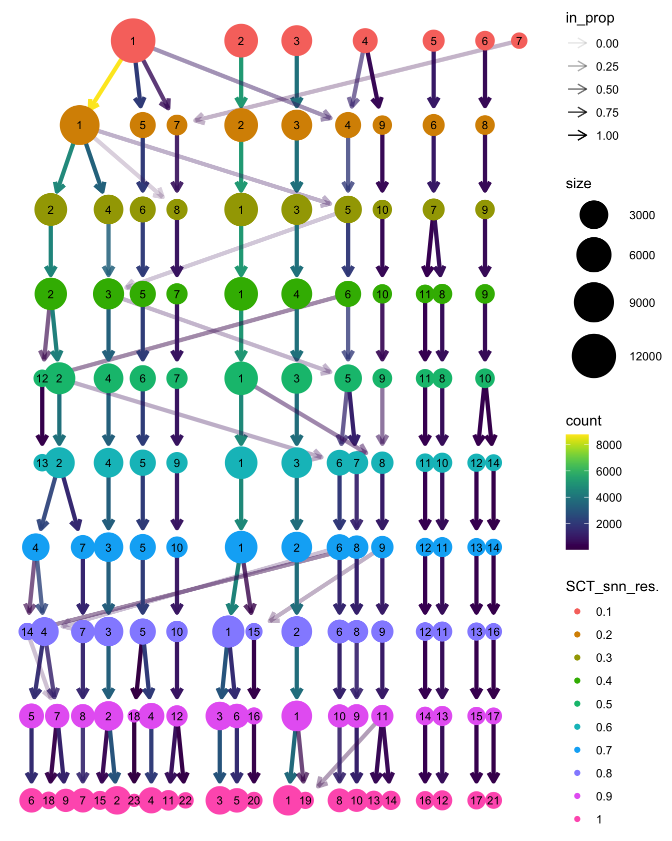
| Version | Author | Date |
|---|---|---|
| 6c36b3e | Jovana Maksimovic | 2026-07-16 |
Identify the two diagnosis clones
BoneMarrowMap projects each cell onto a reference bone marrow atlas
and stores the predicted cell type in
predicted_CellType_Broad. In a B-ALL sample, leukaemic
blasts map onto B-cell progenitor reference states (Pro-B, Pre-B,
HSC-like, etc.), while normal haematopoietic bystander cells map onto
their expected lineages. We use this to separate blasts from normal BM,
then split diagnosis blasts by Leiden cluster identity to define Clone A
and Clone B.
# ── Inspect metadata to confirm available columns ---------------------------- #
cat("Available metadata columns:\n")
Available metadata columns:cat(paste(colnames(seu_c1437@meta.data), collapse = "\n"), "\n\n")orig.ident
nCount_RNA
nFeature_RNA
Sample
Barcode
sizeFactor
PPID
timepoint
status
percent_blasts_in_bone_marrow
final_labelling
sample_name_for_single.cell
batch
patient_timepoint
sum
detected
subsets_is_mito_sum
subsets_is_mito_detected
subsets_is_mito_percent
total
fusion_detected
mito_keep
gene_keep
keep_all
scDblFinder.class
scDblFinder.score
scDblFinder.weighted
scDblFinder.cxds_score
patient_fusion
mapping_error_score
mapping_error_QC
initial_CellType_prob
initial_CellType
predicted_CellType
predicted_CellType_prob
predicted_CellType_Broad
predicted_CellType_No_Abbreviations
initial_Pseudotime
predicted_Pseudotime
nCount_SCT
nFeature_SCT
SCT_snn_res.0.1
SCT_snn_res.0.2
SCT_snn_res.0.3
SCT_snn_res.0.4
SCT_snn_res.0.5
SCT_snn_res.0.6
SCT_snn_res.0.7
SCT_snn_res.0.8
SCT_snn_res.0.9
SCT_snn_res.1
seurat_clusters cat("patient_timepoint breakdown:\n")patient_timepoint breakdown:print(table(seu_c1437$patient_timepoint))
C1437_Diagnosis   C1437_Relapse
          10609           14091
cat("\npredicted_CellType_Broad × patient_timepoint:\n")
predicted_CellType_Broad × patient_timepoint:print(table(seu_c1437$predicted_CellType_Broad, seu_c1437$patient_timepoint))
                       C1437_Diagnosis C1437_Relapse
  B                                196           769
  CD4 Memory T                      84            22
  CD8 Memory T                     249            58
  cDC                                0             3
  Cycling Progenitor                 6             4
  Early Erythroid                   19            11
  Early GMP                         23             7
  Early Lymphoid                   252           678
  EoBasoMast Precursor               1             5
  HSC MPP                            7            27
  Late Erythroid                     8             8
  Late GMP                           1             2
  LMPP                              18             8
  MEP                                3             8
  Monocyte                          94            37
  Naive T                          154            18
  NK                               158           156
  pDC                                0            29
  Plasma Cell                        2            17
  Pre-B                           1190          2278
  Pro-B                           7894          9721
  Pro-Monocyte                       2             9
  Stromal                            0             5
# ── Step 1: define blast-like BoneMarrowMap labels --------------------------- #
# Core blasts: Pro-B, Pre-B (overwhelmingly dominant; unambiguously blast)
# Early Lymphoid is ambiguous — set include_early_lymphoid = TRUE to include.
include_early_lymphoid <- FALSE # ← change to TRUE if you want to include them
blast_types <- c("Pro-B", "Pre-B")
if (include_early_lymphoid) blast_types <- c(blast_types, "Early Lymphoid")
cat("BoneMarrowMap labels classified as blast-like:\n")BoneMarrowMap labels classified as blast-like:print(blast_types)[1] "Pro-B" "Pre-B"# ── Step 2: majority-vote each Leiden cluster as blast/normal by timepoint --- #
# For each cluster: if >50% of cells carry a blast-like BoneMarrowMap label it
# is a blast cluster; otherwise Normal BM. Among blast clusters the majority
# timepoint distinguishes Diagnosis from Relapse blasts.
cluster_votes <- seu_c1437@meta.data %>%
as.data.frame() %>%
rownames_to_column("cell_id") %>%
select(cell_id, predicted_CellType_Broad, SCT_snn_res.0.3, patient_timepoint) %>%
mutate(is_blast = predicted_CellType_Broad %in% blast_types) %>%
group_by(SCT_snn_res.0.3) %>%
summarise(
n_cells = n(),
pct_blast = mean(is_blast),
maj_tp = names(sort(table(patient_timepoint), decreasing = TRUE))[1],
.groups = "drop"
) %>%
mutate(
cluster_class = case_when(
pct_blast > 0.5 & maj_tp == "C1437_Diagnosis" ~ "Diagnosis blast",
pct_blast > 0.5 & maj_tp == "C1437_Relapse" ~ "Relapse blast",
TRUE ~ "Normal BM"
)
)
cat("\nCluster classification (majority BoneMarrowMap vote):\n")
Cluster classification (majority BoneMarrowMap vote):print(cluster_votes)# A tibble: 10 × 5
SCT_snn_res.0.3 n_cells pct_blast maj_tp cluster_class
<fct> <int> <dbl> <chr> <chr>
1 1 5221 0.907 C1437_Diagnosis Diagnosis blast
2 2 4753 0.888 C1437_Relapse Relapse blast
3 3 3875 0.993 C1437_Diagnosis Diagnosis blast
4 4 3382 0.802 C1437_Relapse Relapse blast
5 5 2581 0.979 C1437_Relapse Relapse blast
6 6 2060 0.914 C1437_Relapse Relapse blast
7 7 989 0.00607 C1437_Diagnosis Normal BM
8 8 809 0.828 C1437_Relapse Relapse blast
9 9 531 0.00565 C1437_Diagnosis Normal BM
10 10 499 0.960 C1437_Diagnosis Diagnosis blast# ── Step 3: rank diagnosis blast clusters by size to define Clone A / B ------ #
# Clone A = largest diagnosis blast cluster; Clone B = second largest.
# Inspect the cluster UMAP and swap if biologically warranted.
diag_blast_clusters <- cluster_votes %>%
filter(cluster_class == "Diagnosis blast") %>%
arrange(desc(n_cells))
cat("\nDiagnosis blast clusters (largest → smallest):\n")
Diagnosis blast clusters (largest → smallest):print(diag_blast_clusters)# A tibble: 3 × 5
SCT_snn_res.0.3 n_cells pct_blast maj_tp cluster_class
<fct> <int> <dbl> <chr> <chr>
1 1 5221 0.907 C1437_Diagnosis Diagnosis blast
2 3 3875 0.993 C1437_Diagnosis Diagnosis blast
3 10 499 0.960 C1437_Diagnosis Diagnosis blastcloneA_clusters <- diag_blast_clusters$SCT_snn_res.0.3[1]
cloneB_clusters <- diag_blast_clusters$SCT_snn_res.0.3[2]
relapse_clusters <- cluster_votes %>%
filter(cluster_class == "Relapse blast") %>%
pull(SCT_snn_res.0.3)
cat(glue("\nClone A cluster(s): {paste(cloneA_clusters, collapse=', ')}\n"))Clone A cluster(s): 1cat(glue("Clone B cluster(s): {paste(cloneB_clusters, collapse=', ')}\n"))Clone B cluster(s): 3cat(glue("Relapse cluster(s): {paste(relapse_clusters, collapse=', ')}\n"))Relapse cluster(s): 2, 4, 5, 6, 8# ── Step 4: build cluster → clone lookup and assign to Seurat object --------- #
cluster_to_clone <- cluster_votes %>%
mutate(clone_refined = case_when(
SCT_snn_res.0.3 %in% cloneA_clusters ~ "Diagnosis clone A",
SCT_snn_res.0.3 %in% cloneB_clusters ~ "Diagnosis clone B",
cluster_class == "Relapse blast" ~ "Relapse clone",
cluster_class == "Diagnosis blast" ~ "Diagnosis clone A", # fallback: remaining diagnosis blast clusters → A
TRUE ~ "Normal BM"
)) %>%
select(SCT_snn_res.0.3, clone_refined)
seu_c1437$clone_refined <- cluster_to_clone$clone_refined[
match(seu_c1437$SCT_snn_res.0.3, cluster_to_clone$SCT_snn_res.0.3)
]
cat("\nRefined clone assignments:\n")
Refined clone assignments:print(table(seu_c1437$clone_refined))
Diagnosis clone A Diagnosis clone B         Normal BM     Relapse clone
             5720              3875              1520             13585
# Save clone labels so the joint clustering notebook can load them directly
# without re-running the cluster voting logic.
clone_label_dir <- here("output", "differential_expression_analysis", "patient_C1437")
if (!dir.exists(clone_label_dir)) dir.create(clone_label_dir, recursive = TRUE)
data.frame(
barcode = colnames(seu_c1437),
clone_refined = as.character(seu_c1437$clone_refined),
stringsAsFactors = FALSE
) %>%
write.csv(file.path(clone_label_dir, "clone_labels.csv"), row.names = FALSE)
cat("Clone labels saved to output/differential_expression_analysis/patient_C1437/clone_labels.csv\n")Clone labels saved to output/differential_expression_analysis/patient_C1437/clone_labels.csv# Custom ggplot2 approach required to combine colour + fill + shape aesthetics.
# Normal BM is plotted first so blast/clone cells sit on top.
umap_clone_df <- Embeddings(seu_c1437, "umap") %>%
as.data.frame() %>%
setNames(c("UMAP_1", "UMAP_2")) %>%
rownames_to_column("cell") %>%
left_join(
seu_c1437@meta.data %>%
rownames_to_column("cell") %>%
select(cell, clone_refined, predicted_CellType_Broad),
by = "cell"
) %>%
mutate(clone_refined = factor(
clone_refined,
levels = c("Normal BM", "Diagnosis clone A", "Diagnosis clone B", "Relapse clone")
)) %>%
arrange(clone_refined) # Normal BM first → plotted beneath clone cells
# ── Clone centroid labels ---------------------------------------------------- #
clone_label_pos <- umap_clone_df %>%
filter(clone_refined != "Normal BM") %>%
group_by(clone_refined) %>%
summarise(x = median(UMAP_1), y = median(UMAP_2), .groups = "drop") %>%
mutate(label = str_replace(as.character(clone_refined), "clone", "Clone"))
# ── Normal BM broad cell-type labels at centroids (≥ 10 cells) -------------- #
broad_label_map <- c(
"CD8 Memory T" = "T cell",
"CD4 Memory T" = "T cell",
"Naive T" = "T cell",
"CD8 Effector T" = "T cell",
"CD4 T" = "T cell",
"NK" = "NK",
"HSC MPP" = "HSC/MPP",
"HSC" = "HSC/MPP",
"MPP" = "HSC/MPP",
"Pro-Monocyte" = "Monocyte",
"Monocyte" = "Monocyte",
"cDC" = "DC",
"pDC" = "DC",
"B" = "B cell",
"Plasma Cell" = "B cell",
"Plasma" = "B cell"
)
bm_label_pos <- umap_clone_df %>%
filter(clone_refined == "Normal BM") %>%
left_join(
tibble(predicted_CellType_Broad = names(broad_label_map),
broad = unname(broad_label_map)),
by = "predicted_CellType_Broad"
) %>%
filter(!is.na(broad)) %>%
group_by(broad) %>%
summarise(x = median(UMAP_1), y = median(UMAP_2), n = n(), .groups = "drop") %>%
filter(n >= 10) %>%
rename(label = "broad")
ggplot(umap_clone_df,
aes(x = UMAP_1, y = UMAP_2,
colour = clone_refined,
fill = clone_refined,
shape = clone_refined)) +
geom_point(size = 1.2, stroke = 0.2) +
scale_colour_manual(values = clone_border_cols, guide = "none") +
scale_fill_manual(values = clone_fills, guide = "none") +
scale_shape_manual(values = clone_shapes, guide = "none") +
# Clone labels — larger, bold, dark, white halo for readability
ggrepel::geom_text_repel(
data = clone_label_pos,
aes(x = x, y = y, label = label),
inherit.aes = FALSE,
size = 3.5,
colour = "grey10",
fontface = "bold",
box.padding = 0.4,
point.padding = 0.2,
max.overlaps = 20,
segment.size = 0.3,
segment.colour = "grey40"
) +
# Normal BM labels — smaller, black
ggrepel::geom_text_repel(
data = bm_label_pos,
aes(x = x, y = y, label = label),
inherit.aes = FALSE,
size = 2.8,
colour = "black",
box.padding = 0.4,
point.padding = 0.2,
max.overlaps = 20,
segment.size = 0.25,
segment.colour = "grey40"
) +
labs(title = NULL) +
theme_void(base_size = 10) +
theme(legend.position = "none") -> fig4_E
fig4_E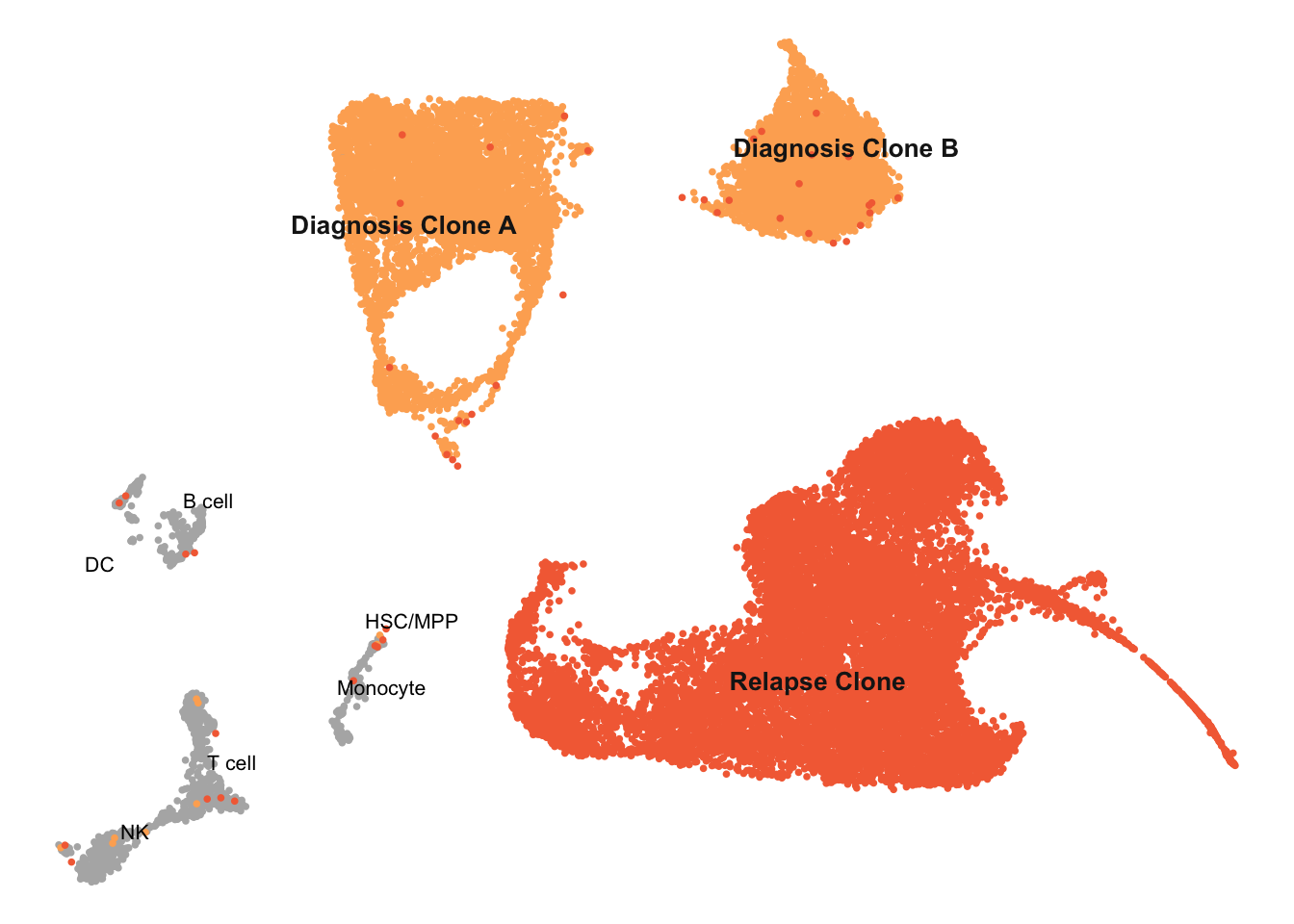
UMAP of C1437 joint diagnosis–relapse object coloured by refined clone identity.
Analysis 1 — C1 / C2 module scoring
Gene sets are derived from Li et al. 2025 Table S3 / Fig. 3 differentially expressed genes between C1 (HSC-like) and C2 (pro-B-like) ETV6::RUNX1 B-ALL. Verify these lists against the published supplementary tables before finalising.
# ── C1 signature (HSC-like; upregulated in C1 relative to C2) --------------- #
# GATA2, CD34, AVP, MECOM, HOXA9, FLT3, SPINK2, MLLT3, ANGPT1, CDK6^low
# (CDK6 is LOWER in C1 — do NOT include in C1 up-signature)
genes_C1 <- c(
  "GATA2", "CD34", "AVP", "MECOM", "HOXA9", "FLT3",
  "SPINK2", "MLLT3", "ANGPT1", "MPO", "CEBPA",
  "PROM1",   # CD133 — HSC surface marker
  "KIT",     # CD117
  "MEIS1"
)

# ── C2 signature (pro-B-like; upregulated in C2 relative to C1) ------------- #
genes_C2 <- c(
  "PAX5", "EBF1", "CD19", "MS4A1",   # CD20
  "VPREB1", "IGLL1", "CD79A", "CD79B",
  "BLNK", "RAG1", "RAG2",
  "DNTT",    # TdT — active V(D)J recombination
  "MME"      # CD10
)

# ── Filter to genes present in the assay ------------------------------------ #
genes_present <- rownames(seu_c1437)

genes_C1 <- intersect(genes_C1, genes_present)
genes_C2 <- intersect(genes_C2, genes_present)

cat(glue("C1 genes found: {length(genes_C1)} / intended\n"))
C1 genes found: 14 / intendedcat(glue("C2 genes found: {length(genes_C2)} / intended\n"))C2 genes found: 13 / intendedcat("C1:", paste(genes_C1, collapse = ", "), "\n")C1: GATA2, CD34, AVP, MECOM, HOXA9, FLT3, SPINK2, MLLT3, ANGPT1, MPO, CEBPA, PROM1, KIT, MEIS1 cat("C2:", paste(genes_C2, collapse = ", "), "\n")C2: PAX5, EBF1, CD19, MS4A1, VPREB1, IGLL1, CD79A, CD79B, BLNK, RAG1, RAG2, DNTT, MME out_scored <- here("data", "RDS", "ball_exp2_c1437_li2025_scored.seu.rds")
seu_c1437 <- cache_rds(out_scored, {
seu_c1437 <- AddModuleScore(
seu_c1437,
features = list(C1 = genes_C1),
name = "Li2025_C1",
seed = 42
)
seu_c1437 <- AddModuleScore(
seu_c1437,
features = list(C2 = genes_C2),
name = "Li2025_C2",
seed = 42
)
# Composite: C1 − C2 (positive = more C1-like)
seu_c1437$Li2025_C1vsC2 <- seu_c1437$Li2025_C11 - seu_c1437$Li2025_C21
seu_c1437
})
# Re-apply clone labels after cache load (derived from cluster membership)
seu_c1437$clone_refined <- cluster_to_clone$clone_refined[
match(seu_c1437$SCT_snn_res.0.3, cluster_to_clone$SCT_snn_res.0.3)
]Differential expression between clones
Pseudo-bulk–style differential expression using limma-trend with TREAT (|LFC| > log2(1.2) threshold, adj. p < 0.01). Mitochondrial genes and genes expressed in fewer than 100 cells are excluded. All three clone groups are modelled jointly; contrasts extract pairwise comparisons.
keep      <- seu_c1437$clone_refined != "Normal BM"
rawcounts <- DGEList(as.matrix(seu_c1437[["RNA"]]$counts[, keep]))

keep.genes <- !str_detect(rownames(rawcounts), "^MT-") &
  rowSums(rawcounts$counts > 0) > 100

y        <- normCounts(rawcounts[keep.genes, ], log = TRUE, prior.count = 0.5)
clustgrp <- fct_drop(factor(seu_c1437$clone_refined)[keep])

# Cell cycle covariates deliberately excluded: cell cycle activity is part of
# the C1/C2 biological distinction (C2/Clone B is more proliferative) and
# should not be regressed out.
design <- model.matrix(~ 0 + clustgrp)
colnames(design)[seq_along(levels(clustgrp))] <- levels(clustgrp)
colnames(design) <- str_replace_all(colnames(design), " ", "_")

mycont <- makeContrasts(
  DiaAvRel      = Diagnosis_clone_A - Relapse_clone,
  DiaBvRel      = Diagnosis_clone_B - Relapse_clone,
  DiaAvDiaB     = Diagnosis_clone_A - Diagnosis_clone_B,
  # Unique-to-group contrasts: each clone vs the average of the other two.
  # A positive result means the group is specifically higher than the mean
  # of the remaining two groups in a single balanced test.
  CloneA_unique = Diagnosis_clone_A - (Diagnosis_clone_B + Relapse_clone) / 2,
  CloneB_unique = Diagnosis_clone_B - (Diagnosis_clone_A + Relapse_clone) / 2,
  Relapse_unique = Relapse_clone   - (Diagnosis_clone_A + Diagnosis_clone_B) / 2,
  levels    = design
)

fit      <- lmFit(y, design)
fit.cont <- contrasts.fit(fit, contrasts = mycont)
fit.cont <- eBayes(fit.cont, trend = TRUE, robust = TRUE)
tr       <- treat(fit.cont, lfc = log2(fc))

dt <- decideTests(tr)
cat(glue("TREAT DE gene counts (|LFC| > log2({fc}), adj.p < {pval}):\n"))
TREAT DE gene counts (|LFC| > log2(1.2), adj.p < 0.01):print(summary(dt)) DiaAvRel DiaBvRel DiaAvDiaB CloneA_unique CloneB_unique Relapse_unique
Down 250 340 133 132 163 171
NotSig 11081 11090 11266 11279 11302 11143
Up 255 156 187 175 121 272# y, design, and mycont are available from the de-analysis chunk above.
# ── Fetch MSigDB gene sets via msigdbr --------------------------------------- #
# Hallmarks: MYC activity (Clone B proliferative drive), apoptosis resistance
# (Clone A FATE1), and cell cycle programmes
msig_h <- msigdbr(species = "Homo sapiens", category = "H") %>%
filter(gs_name %in% c(
"HALLMARK_MYC_TARGETS_V1",
"HALLMARK_MYC_TARGETS_V2",
"HALLMARK_APOPTOSIS",
"HALLMARK_E2F_TARGETS",
"HALLMARK_G2M_CHECKPOINT"
)) %>%
split(.$gs_name) %>%
lapply(pull, gene_symbol)
# C2 curated: B cell receptor signalling (Clone B BLNK/CD79B),
# glucocorticoid response (Clone B TSC22D3/TXNIP → steroid sensitivity),
# haematopoietic stem cell identity (Clone A HSC programme)
msig_c2 <- msigdbr(species = "Homo sapiens", category = "C2") %>%
filter(
str_detect(gs_name, "B_CELL_RECEPTOR|BCR_SIGNALING|BCR_PATHWAY") |
str_detect(gs_name, "GLUCOCORTICOID") |
str_detect(gs_name, "HEMATOPOIETIC_STEM_CELL")
) %>%
split(.$gs_name) %>%
lapply(pull, gene_symbol)
cat(glue(
"MSigDB sets fetched: {length(msig_h)} Hallmark, {length(msig_c2)} C2 curated\n"
))MSigDB sets fetched: 5 Hallmark, 22 C2 curated# ── Combine all gene sets ---------------------------------------------------- #
gene_sets_cam <- c(
list(
`Li2025 C1 (HSC-like)` = genes_C1,
`Li2025 C2 (pro-B-like)` = genes_C2
),
msig_h,
msig_c2
)
idx_cam <- ids2indices(gene_sets_cam, rownames(y))
# ── Run camera for each contrast --------------------------------------------- #
cam_results <- purrr::imap_dfr(
setNames(colnames(mycont), colnames(mycont)),
function(coef_name, ...) {
camera(y, idx_cam, design, contrast = mycont[, coef_name]) %>%
as_tibble(rownames = "gene_set") %>%
mutate(contrast = coef_name)
}
) %>%
select(contrast, gene_set, NGenes, Direction, PValue, FDR) %>%
mutate(across(c(PValue, FDR), ~signif(.x, 3)))
# ── Display: significant results (FDR < 0.2), sorted by contrast then FDR --- #
cat("camera gene set test — significant results (FDR < 0.2):\n")camera gene set test — significant results (FDR < 0.2):knitr::kable(
cam_results %>% filter(FDR < 0.2) %>% arrange(contrast, FDR),
caption = "camera competitive gene set test",
col.names = c("Contrast", "Gene set", "N genes", "Direction", "P-value", "FDR")
)| Contrast | Gene set | N genes | Direction | P-value | FDR |
|---|---|---|---|---|---|
| CloneA_unique | RHEIN_ALL_GLUCOCORTICOID_THERAPY_UP | 55 | Down | 2.40e-06 | 3.54e-05 |
| CloneA_unique | WP_HEMATOPOIETIC_STEM_CELL_DIFFERENTIATION | 38 | Down | 2.50e-06 | 3.54e-05 |
| CloneA_unique | OSWALD_HEMATOPOIETIC_STEM_CELL_IN_COLLAGEN_GEL_UP | 157 | Down | 4.40e-06 | 4.09e-05 |
| CloneA_unique | HALLMARK_APOPTOSIS | 126 | Down | 1.50e-03 | 1.05e-02 |
| CloneA_unique | HALLMARK_MYC_TARGETS_V1 | 167 | Up | 8.27e-03 | 4.63e-02 |
| CloneA_unique | DEBOSSCHER_NFKB_TARGETS_REPRESSED_BY_GLUCOCORTICOIDS | 6 | Down | 1.44e-02 | 6.71e-02 |
| CloneA_unique | SA_B_CELL_RECEPTOR_COMPLEXES | 21 | Down | 2.35e-02 | 9.39e-02 |
| CloneA_unique | KEGG_B_CELL_RECEPTOR_SIGNALING_PATHWAY | 69 | Down | 2.91e-02 | 9.70e-02 |
| CloneA_unique | HALLMARK_E2F_TARGETS | 193 | Up | 3.12e-02 | 9.70e-02 |
| CloneA_unique | WP_GLUCOCORTICOID_RECEPTOR_PATHWAY | 44 | Down | 4.12e-02 | 1.13e-01 |
| CloneA_unique | RHEIN_ALL_GLUCOCORTICOID_THERAPY_DN | 337 | Up | 4.45e-02 | 1.13e-01 |
| CloneA_unique | Li2025 C2 (pro-B-like) | 13 | Down | 6.47e-02 | 1.45e-01 |
| CloneA_unique | JAATINEN_HEMATOPOIETIC_STEM_CELL_DN | 114 | Down | 6.74e-02 | 1.45e-01 |
| CloneA_unique | REACTOME_RUNX1_REGULATES_TRANSCRIPTION_OF_GENES_INVOLVED_IN_BCR_SIGNALING | 6 | Down | 7.57e-02 | 1.51e-01 |
| CloneA_unique | JAATINEN_HEMATOPOIETIC_STEM_CELL_UP | 226 | Up | 8.41e-02 | 1.57e-01 |
| CloneA_unique | HALLMARK_G2M_CHECKPOINT | 185 | Up | 9.77e-02 | 1.62e-01 |
| CloneA_unique | REACTOME_ANTIGEN_ACTIVATES_B_CELL_RECEPTOR_BCR_LEADING_TO_GENERATION_OF_SECOND_MESSENGERS | 32 | Down | 9.81e-02 | 1.62e-01 |
| CloneB_unique | HALLMARK_E2F_TARGETS | 193 | Down | 0.00e+00 | 0.00e+00 |
| CloneB_unique | HALLMARK_MYC_TARGETS_V2 | 55 | Down | 0.00e+00 | 0.00e+00 |
| CloneB_unique | HALLMARK_MYC_TARGETS_V1 | 167 | Down | 0.00e+00 | 1.00e-07 |
| CloneB_unique | Li2025 C2 (pro-B-like) | 13 | Up | 0.00e+00 | 1.00e-07 |
| CloneB_unique | HALLMARK_G2M_CHECKPOINT | 185 | Down | 2.00e-07 | 1.20e-06 |
| CloneB_unique | RHEIN_ALL_GLUCOCORTICOID_THERAPY_DN | 337 | Down | 1.87e-03 | 8.28e-03 |
| CloneB_unique | KEGG_B_CELL_RECEPTOR_SIGNALING_PATHWAY | 69 | Up | 2.07e-03 | 8.28e-03 |
| CloneB_unique | OSWALD_HEMATOPOIETIC_STEM_CELL_IN_COLLAGEN_GEL_DN | 213 | Up | 2.45e-03 | 8.57e-03 |
| CloneB_unique | REACTOME_ANTIGEN_ACTIVATES_B_CELL_RECEPTOR_BCR_LEADING_TO_GENERATION_OF_SECOND_MESSENGERS | 32 | Up | 1.68e-02 | 5.06e-02 |
| CloneB_unique | BIOCARTA_BCR_PATHWAY | 33 | Up | 1.81e-02 | 5.06e-02 |
| CloneB_unique | DEBOSSCHER_NFKB_TARGETS_REPRESSED_BY_GLUCOCORTICOIDS | 6 | Down | 4.79e-02 | 1.14e-01 |
| CloneB_unique | RHEIN_ALL_GLUCOCORTICOID_THERAPY_UP | 55 | Up | 4.89e-02 | 1.14e-01 |
| CloneB_unique | WP_B_CELL_RECEPTOR_SIGNALING | 90 | Up | 5.54e-02 | 1.19e-01 |
| CloneB_unique | OSWALD_HEMATOPOIETIC_STEM_CELL_IN_COLLAGEN_GEL_UP | 157 | Down | 6.09e-02 | 1.22e-01 |
| DiaAvDiaB | HALLMARK_E2F_TARGETS | 193 | Up | 1.00e-07 | 3.30e-06 |
| DiaAvDiaB | HALLMARK_MYC_TARGETS_V1 | 167 | Up | 7.00e-07 | 9.20e-06 |
| DiaAvDiaB | Li2025 C2 (pro-B-like) | 13 | Down | 8.70e-06 | 8.13e-05 |
| DiaAvDiaB | RHEIN_ALL_GLUCOCORTICOID_THERAPY_UP | 55 | Down | 2.83e-05 | 1.98e-04 |
| DiaAvDiaB | HALLMARK_G2M_CHECKPOINT | 185 | Up | 6.24e-05 | 3.49e-04 |
| DiaAvDiaB | HALLMARK_MYC_TARGETS_V2 | 55 | Up | 1.73e-04 | 8.07e-04 |
| DiaAvDiaB | KEGG_B_CELL_RECEPTOR_SIGNALING_PATHWAY | 69 | Down | 1.55e-03 | 6.19e-03 |
| DiaAvDiaB | RHEIN_ALL_GLUCOCORTICOID_THERAPY_DN | 337 | Up | 2.18e-03 | 7.62e-03 |
| DiaAvDiaB | WP_HEMATOPOIETIC_STEM_CELL_DIFFERENTIATION | 38 | Down | 4.08e-03 | 1.27e-02 |
| DiaAvDiaB | REACTOME_ANTIGEN_ACTIVATES_B_CELL_RECEPTOR_BCR_LEADING_TO_GENERATION_OF_SECOND_MESSENGERS | 32 | Down | 1.50e-02 | 4.21e-02 |
| DiaAvDiaB | WP_GLUCOCORTICOID_RECEPTOR_PATHWAY | 44 | Down | 3.89e-02 | 9.89e-02 |
| DiaAvDiaB | HALLMARK_APOPTOSIS | 126 | Down | 4.24e-02 | 9.89e-02 |
| DiaAvDiaB | OSWALD_HEMATOPOIETIC_STEM_CELL_IN_COLLAGEN_GEL_UP | 157 | Down | 5.30e-02 | 1.11e-01 |
| DiaAvDiaB | OSWALD_HEMATOPOIETIC_STEM_CELL_IN_COLLAGEN_GEL_DN | 213 | Down | 5.77e-02 | 1.11e-01 |
| DiaAvDiaB | SA_B_CELL_RECEPTOR_COMPLEXES | 21 | Down | 5.97e-02 | 1.11e-01 |
| DiaAvDiaB | BIOCARTA_BCR_PATHWAY | 33 | Down | 7.31e-02 | 1.23e-01 |
| DiaAvDiaB | REACTOME_RUNX1_REGULATES_TRANSCRIPTION_OF_GENES_INVOLVED_IN_BCR_SIGNALING | 6 | Down | 7.72e-02 | 1.23e-01 |
| DiaAvDiaB | JAATINEN_HEMATOPOIETIC_STEM_CELL_UP | 226 | Up | 8.21e-02 | 1.23e-01 |
| DiaAvDiaB | WP_B_CELL_RECEPTOR_SIGNALING | 90 | Down | 8.35e-02 | 1.23e-01 |
| DiaAvDiaB | JAATINEN_HEMATOPOIETIC_STEM_CELL_DN | 114 | Down | 1.21e-01 | 1.69e-01 |
| DiaAvRel | OSWALD_HEMATOPOIETIC_STEM_CELL_IN_COLLAGEN_GEL_UP | 157 | Down | 0.00e+00 | 5.00e-07 |
| DiaAvRel | WP_HEMATOPOIETIC_STEM_CELL_DIFFERENTIATION | 38 | Down | 4.00e-07 | 5.90e-06 |
| DiaAvRel | RHEIN_ALL_GLUCOCORTICOID_THERAPY_UP | 55 | Down | 4.60e-05 | 4.29e-04 |
| DiaAvRel | DEBOSSCHER_NFKB_TARGETS_REPRESSED_BY_GLUCOCORTICOIDS | 6 | Down | 4.89e-04 | 3.42e-03 |
| DiaAvRel | HALLMARK_APOPTOSIS | 126 | Down | 7.31e-04 | 4.10e-03 |
| DiaAvRel | HALLMARK_MYC_TARGETS_V2 | 55 | Down | 1.85e-02 | 8.62e-02 |
| DiaAvRel | SA_B_CELL_RECEPTOR_COMPLEXES | 21 | Down | 4.16e-02 | 1.66e-01 |
| DiaBvRel | HALLMARK_MYC_TARGETS_V2 | 55 | Down | 0.00e+00 | 0.00e+00 |
| DiaBvRel | HALLMARK_E2F_TARGETS | 193 | Down | 0.00e+00 | 1.00e-07 |
| DiaBvRel | Li2025 C2 (pro-B-like) | 13 | Up | 2.30e-06 | 2.11e-05 |
| DiaBvRel | OSWALD_HEMATOPOIETIC_STEM_CELL_IN_COLLAGEN_GEL_UP | 157 | Down | 4.00e-06 | 2.81e-05 |
| DiaBvRel | HALLMARK_G2M_CHECKPOINT | 185 | Down | 1.28e-05 | 6.04e-05 |
| DiaBvRel | HALLMARK_MYC_TARGETS_V1 | 167 | Down | 1.29e-05 | 6.04e-05 |
| DiaBvRel | DEBOSSCHER_NFKB_TARGETS_REPRESSED_BY_GLUCOCORTICOIDS | 6 | Down | 4.87e-04 | 1.95e-03 |
| DiaBvRel | WP_HEMATOPOIETIC_STEM_CELL_DIFFERENTIATION | 38 | Down | 2.19e-03 | 7.66e-03 |
| DiaBvRel | OSWALD_HEMATOPOIETIC_STEM_CELL_IN_COLLAGEN_GEL_DN | 213 | Up | 3.20e-03 | 9.94e-03 |
| DiaBvRel | BIOCARTA_BCR_PATHWAY | 33 | Up | 4.19e-02 | 1.14e-01 |
| DiaBvRel | RHEIN_ALL_GLUCOCORTICOID_THERAPY_DN | 337 | Down | 4.47e-02 | 1.14e-01 |
| DiaBvRel | HALLMARK_APOPTOSIS | 126 | Down | 5.21e-02 | 1.21e-01 |
| DiaBvRel | KEGG_B_CELL_RECEPTOR_SIGNALING_PATHWAY | 69 | Up | 6.01e-02 | 1.29e-01 |
| Relapse_unique | OSWALD_HEMATOPOIETIC_STEM_CELL_IN_COLLAGEN_GEL_UP | 157 | Up | 0.00e+00 | 5.00e-07 |
| Relapse_unique | HALLMARK_MYC_TARGETS_V2 | 55 | Up | 6.10e-06 | 7.31e-05 |
| Relapse_unique | WP_HEMATOPOIETIC_STEM_CELL_DIFFERENTIATION | 38 | Up | 7.80e-06 | 7.31e-05 |
| Relapse_unique | DEBOSSCHER_NFKB_TARGETS_REPRESSED_BY_GLUCOCORTICOIDS | 6 | Up | 1.28e-04 | 8.94e-04 |
| Relapse_unique | HALLMARK_E2F_TARGETS | 193 | Up | 4.13e-04 | 2.31e-03 |
| Relapse_unique | HALLMARK_APOPTOSIS | 126 | Up | 3.04e-03 | 1.42e-02 |
| Relapse_unique | Li2025 C2 (pro-B-like) | 13 | Down | 4.87e-03 | 1.95e-02 |
| Relapse_unique | RHEIN_ALL_GLUCOCORTICOID_THERAPY_UP | 55 | Up | 5.75e-03 | 2.01e-02 |
| Relapse_unique | HALLMARK_G2M_CHECKPOINT | 185 | Up | 8.61e-03 | 2.68e-02 |
| Relapse_unique | OSWALD_HEMATOPOIETIC_STEM_CELL_IN_COLLAGEN_GEL_DN | 213 | Down | 2.91e-02 | 7.49e-02 |
| Relapse_unique | HALLMARK_MYC_TARGETS_V1 | 167 | Up | 2.94e-02 | 7.49e-02 |
cat("\nFull results:\n")
Full results:print(cam_results %>% arrange(contrast, FDR), n = Inf)# A tibble: 168 × 6
contrast gene_set NGenes Direction PValue FDR
<chr> <chr> <dbl> <chr> <dbl> <dbl>
1 CloneA_unique RHEIN_ALL_GLUCOCORTICOID_… 55 Down 2.41e- 6 3.54e- 5
2 CloneA_unique WP_HEMATOPOIETIC_STEM_CEL… 38 Down 2.53e- 6 3.54e- 5
3 CloneA_unique OSWALD_HEMATOPOIETIC_STEM… 157 Down 4.38e- 6 4.09e- 5
4 CloneA_unique HALLMARK_APOPTOSIS 126 Down 1.5 e- 3 1.05e- 2
5 CloneA_unique HALLMARK_MYC_TARGETS_V1 167 Up 8.27e- 3 4.63e- 2
6 CloneA_unique DEBOSSCHER_NFKB_TARGETS_R… 6 Down 1.44e- 2 6.71e- 2
7 CloneA_unique SA_B_CELL_RECEPTOR_COMPLE… 21 Down 2.35e- 2 9.39e- 2
8 CloneA_unique KEGG_B_CELL_RECEPTOR_SIGN… 69 Down 2.91e- 2 9.7 e- 2
9 CloneA_unique HALLMARK_E2F_TARGETS 193 Up 3.12e- 2 9.7 e- 2
10 CloneA_unique WP_GLUCOCORTICOID_RECEPTO… 44 Down 4.12e- 2 1.13e- 1
11 CloneA_unique RHEIN_ALL_GLUCOCORTICOID_… 337 Up 4.45e- 2 1.13e- 1
12 CloneA_unique Li2025 C2 (pro-B-like) 13 Down 6.47e- 2 1.45e- 1
13 CloneA_unique JAATINEN_HEMATOPOIETIC_ST… 114 Down 6.74e- 2 1.45e- 1
14 CloneA_unique REACTOME_RUNX1_REGULATES_… 6 Down 7.57e- 2 1.51e- 1
15 CloneA_unique JAATINEN_HEMATOPOIETIC_ST… 226 Up 8.41e- 2 1.57e- 1
16 CloneA_unique HALLMARK_G2M_CHECKPOINT 185 Up 9.77e- 2 1.62e- 1
17 CloneA_unique REACTOME_ANTIGEN_ACTIVATE… 32 Down 9.81e- 2 1.62e- 1
18 CloneA_unique REACTOME_DOWNSTREAM_SIGNA… 65 Up 2.76e- 1 4.29e- 1
19 CloneA_unique WP_B_CELL_RECEPTOR_SIGNAL… 90 Down 3.2 e- 1 4.71e- 1
20 CloneA_unique BIOCARTA_BCR_PATHWAY 33 Down 4.85e- 1 6.79e- 1
21 CloneA_unique WP_CLASSICAL_PATHWAY_OF_S… 3 Down 5.6 e- 1 7.36e- 1
22 CloneA_unique WP_GLUCOCORTICOID_BIOSYNT… 4 Up 5.98e- 1 7.36e- 1
23 CloneA_unique WP_HEMATOPOIETIC_STEM_CEL… 19 Down 6.17e- 1 7.36e- 1
24 CloneA_unique SIG_BCR_SIGNALING_PATHWAY 44 Down 6.31e- 1 7.36e- 1
25 CloneA_unique HALLMARK_MYC_TARGETS_V2 55 Up 6.59e- 1 7.38e- 1
26 CloneA_unique OSWALD_HEMATOPOIETIC_STEM… 213 Down 7.91e- 1 8.52e- 1
27 CloneA_unique REACTOME_SIGNALING_BY_THE… 96 Down 9.75e- 1 9.81e- 1
28 CloneA_unique Li2025 C1 (HSC-like) 9 Up 9.81e- 1 9.81e- 1
29 CloneB_unique HALLMARK_E2F_TARGETS 193 Down 5.12e-12 1.43e-10
30 CloneB_unique HALLMARK_MYC_TARGETS_V2 55 Down 8.34e-10 1.17e- 8
31 CloneB_unique HALLMARK_MYC_TARGETS_V1 167 Down 8.73e- 9 8.15e- 8
32 CloneB_unique Li2025 C2 (pro-B-like) 13 Up 1.21e- 8 8.44e- 8
33 CloneB_unique HALLMARK_G2M_CHECKPOINT 185 Down 2.19e- 7 1.22e- 6
34 CloneB_unique RHEIN_ALL_GLUCOCORTICOID_… 337 Down 1.87e- 3 8.28e- 3
35 CloneB_unique KEGG_B_CELL_RECEPTOR_SIGN… 69 Up 2.07e- 3 8.28e- 3
36 CloneB_unique OSWALD_HEMATOPOIETIC_STEM… 213 Up 2.45e- 3 8.57e- 3
37 CloneB_unique REACTOME_ANTIGEN_ACTIVATE… 32 Up 1.68e- 2 5.06e- 2
38 CloneB_unique BIOCARTA_BCR_PATHWAY 33 Up 1.81e- 2 5.06e- 2
39 CloneB_unique DEBOSSCHER_NFKB_TARGETS_R… 6 Down 4.79e- 2 1.14e- 1
40 CloneB_unique RHEIN_ALL_GLUCOCORTICOID_… 55 Up 4.89e- 2 1.14e- 1
41 CloneB_unique WP_B_CELL_RECEPTOR_SIGNAL… 90 Up 5.54e- 2 1.19e- 1
42 CloneB_unique OSWALD_HEMATOPOIETIC_STEM… 157 Down 6.09e- 2 1.22e- 1
43 CloneB_unique Li2025 C1 (HSC-like) 9 Down 1.37e- 1 2.56e- 1
44 CloneB_unique REACTOME_SIGNALING_BY_THE… 96 Up 1.66e- 1 2.9 e- 1
45 CloneB_unique WP_GLUCOCORTICOID_RECEPTO… 44 Up 1.9 e- 1 3.13e- 1
46 CloneB_unique SIG_BCR_SIGNALING_PATHWAY 44 Up 2.63e- 1 4 e- 1
47 CloneB_unique JAATINEN_HEMATOPOIETIC_ST… 226 Down 2.75e- 1 4 e- 1
48 CloneB_unique REACTOME_RUNX1_REGULATES_… 6 Up 2.86e- 1 4 e- 1
49 CloneB_unique SA_B_CELL_RECEPTOR_COMPLE… 21 Up 4.74e- 1 6.28e- 1
50 CloneB_unique WP_HEMATOPOIETIC_STEM_CEL… 19 Up 5.12e- 1 6.28e- 1
51 CloneB_unique JAATINEN_HEMATOPOIETIC_ST… 114 Up 5.16e- 1 6.28e- 1
52 CloneB_unique WP_HEMATOPOIETIC_STEM_CEL… 38 Down 7.4 e- 1 8.63e- 1
53 CloneB_unique REACTOME_DOWNSTREAM_SIGNA… 65 Up 8.11e- 1 9.08e- 1
54 CloneB_unique WP_CLASSICAL_PATHWAY_OF_S… 3 Down 8.51e- 1 9.15e- 1
55 CloneB_unique WP_GLUCOCORTICOID_BIOSYNT… 4 Up 8.83e- 1 9.15e- 1
56 CloneB_unique HALLMARK_APOPTOSIS 126 Down 9.47e- 1 9.47e- 1
57 DiaAvDiaB HALLMARK_E2F_TARGETS 193 Up 1.16e- 7 3.26e- 6
58 DiaAvDiaB HALLMARK_MYC_TARGETS_V1 167 Up 6.56e- 7 9.18e- 6
59 DiaAvDiaB Li2025 C2 (pro-B-like) 13 Down 8.72e- 6 8.13e- 5
60 DiaAvDiaB RHEIN_ALL_GLUCOCORTICOID_… 55 Down 2.83e- 5 1.98e- 4
61 DiaAvDiaB HALLMARK_G2M_CHECKPOINT 185 Up 6.24e- 5 3.49e- 4
62 DiaAvDiaB HALLMARK_MYC_TARGETS_V2 55 Up 1.73e- 4 8.07e- 4
63 DiaAvDiaB KEGG_B_CELL_RECEPTOR_SIGN… 69 Down 1.55e- 3 6.19e- 3
64 DiaAvDiaB RHEIN_ALL_GLUCOCORTICOID_… 337 Up 2.18e- 3 7.62e- 3
65 DiaAvDiaB WP_HEMATOPOIETIC_STEM_CEL… 38 Down 4.08e- 3 1.27e- 2
66 DiaAvDiaB REACTOME_ANTIGEN_ACTIVATE… 32 Down 1.5 e- 2 4.21e- 2
67 DiaAvDiaB WP_GLUCOCORTICOID_RECEPTO… 44 Down 3.89e- 2 9.89e- 2
68 DiaAvDiaB HALLMARK_APOPTOSIS 126 Down 4.24e- 2 9.89e- 2
69 DiaAvDiaB OSWALD_HEMATOPOIETIC_STEM… 157 Down 5.3 e- 2 1.11e- 1
70 DiaAvDiaB OSWALD_HEMATOPOIETIC_STEM… 213 Down 5.77e- 2 1.11e- 1
71 DiaAvDiaB SA_B_CELL_RECEPTOR_COMPLE… 21 Down 5.97e- 2 1.11e- 1
72 DiaAvDiaB BIOCARTA_BCR_PATHWAY 33 Down 7.31e- 2 1.23e- 1
73 DiaAvDiaB REACTOME_RUNX1_REGULATES_… 6 Down 7.72e- 2 1.23e- 1
74 DiaAvDiaB JAATINEN_HEMATOPOIETIC_ST… 226 Up 8.21e- 2 1.23e- 1
75 DiaAvDiaB WP_B_CELL_RECEPTOR_SIGNAL… 90 Down 8.35e- 2 1.23e- 1
76 DiaAvDiaB JAATINEN_HEMATOPOIETIC_ST… 114 Down 1.21e- 1 1.69e- 1
77 DiaAvDiaB SIG_BCR_SIGNALING_PATHWAY 44 Down 3.46e- 1 4.61e- 1
78 DiaAvDiaB Li2025 C1 (HSC-like) 9 Up 3.93e- 1 5 e- 1
79 DiaAvDiaB REACTOME_SIGNALING_BY_THE… 96 Down 4.2 e- 1 5.12e- 1
80 DiaAvDiaB WP_HEMATOPOIETIC_STEM_CEL… 19 Down 4.87e- 1 5.68e- 1
81 DiaAvDiaB REACTOME_DOWNSTREAM_SIGNA… 65 Up 5.66e- 1 6.34e- 1
82 DiaAvDiaB DEBOSSCHER_NFKB_TARGETS_R… 6 Down 6.32e- 1 6.81e- 1
83 DiaAvDiaB WP_CLASSICAL_PATHWAY_OF_S… 3 Down 7.84e- 1 7.95e- 1
84 DiaAvDiaB WP_GLUCOCORTICOID_BIOSYNT… 4 Up 7.95e- 1 7.95e- 1
85 DiaAvRel OSWALD_HEMATOPOIETIC_STEM… 157 Down 1.64e- 8 4.59e- 7
86 DiaAvRel WP_HEMATOPOIETIC_STEM_CEL… 38 Down 4.18e- 7 5.86e- 6
87 DiaAvRel RHEIN_ALL_GLUCOCORTICOID_… 55 Down 4.6 e- 5 4.29e- 4
88 DiaAvRel DEBOSSCHER_NFKB_TARGETS_R… 6 Down 4.89e- 4 3.42e- 3
89 DiaAvRel HALLMARK_APOPTOSIS 126 Down 7.31e- 4 4.1 e- 3
90 DiaAvRel HALLMARK_MYC_TARGETS_V2 55 Down 1.85e- 2 8.62e- 2
91 DiaAvRel SA_B_CELL_RECEPTOR_COMPLE… 21 Down 4.16e- 2 1.66e- 1
92 DiaAvRel JAATINEN_HEMATOPOIETIC_ST… 114 Down 1 e- 1 3.5 e- 1
93 DiaAvRel WP_GLUCOCORTICOID_RECEPTO… 44 Down 1.18e- 1 3.67e- 1
94 DiaAvRel REACTOME_RUNX1_REGULATES_… 6 Down 1.68e- 1 4.63e- 1
95 DiaAvRel JAATINEN_HEMATOPOIETIC_ST… 226 Up 1.82e- 1 4.63e- 1
96 DiaAvRel REACTOME_DOWNSTREAM_SIGNA… 65 Up 2.09e- 1 4.88e- 1
97 DiaAvRel OSWALD_HEMATOPOIETIC_STEM… 213 Up 2.6 e- 1 5.59e- 1
98 DiaAvRel KEGG_B_CELL_RECEPTOR_SIGN… 69 Down 3.75e- 1 6.75e- 1
99 DiaAvRel HALLMARK_E2F_TARGETS 193 Down 3.8 e- 1 6.75e- 1
100 DiaAvRel RHEIN_ALL_GLUCOCORTICOID_… 337 Up 4.76e- 1 6.75e- 1
101 DiaAvRel WP_CLASSICAL_PATHWAY_OF_S… 3 Down 4.81e- 1 6.75e- 1
102 DiaAvRel REACTOME_ANTIGEN_ACTIVATE… 32 Down 5.05e- 1 6.75e- 1
103 DiaAvRel Li2025 C2 (pro-B-like) 13 Up 5.06e- 1 6.75e- 1
104 DiaAvRel Li2025 C1 (HSC-like) 9 Down 5.16e- 1 6.75e- 1
105 DiaAvRel WP_GLUCOCORTICOID_BIOSYNT… 4 Up 5.33e- 1 6.75e- 1
106 DiaAvRel HALLMARK_G2M_CHECKPOINT 185 Down 5.34e- 1 6.75e- 1
107 DiaAvRel REACTOME_SIGNALING_BY_THE… 96 Up 5.55e- 1 6.75e- 1
108 DiaAvRel BIOCARTA_BCR_PATHWAY 33 Up 7.17e- 1 8.37e- 1
109 DiaAvRel WP_HEMATOPOIETIC_STEM_CEL… 19 Down 8.24e- 1 9.14e- 1
110 DiaAvRel WP_B_CELL_RECEPTOR_SIGNAL… 90 Down 8.55e- 1 9.14e- 1
111 DiaAvRel HALLMARK_MYC_TARGETS_V1 167 Up 8.81e- 1 9.14e- 1
112 DiaAvRel SIG_BCR_SIGNALING_PATHWAY 44 Down 9.99e- 1 9.99e- 1
113 DiaBvRel HALLMARK_MYC_TARGETS_V2 55 Down 1.28e- 9 3.59e- 8
114 DiaBvRel HALLMARK_E2F_TARGETS 193 Down 5.55e- 9 7.78e- 8
115 DiaBvRel Li2025 C2 (pro-B-like) 13 Up 2.26e- 6 2.11e- 5
116 DiaBvRel OSWALD_HEMATOPOIETIC_STEM… 157 Down 4.01e- 6 2.81e- 5
117 DiaBvRel HALLMARK_G2M_CHECKPOINT 185 Down 1.28e- 5 6.04e- 5
118 DiaBvRel HALLMARK_MYC_TARGETS_V1 167 Down 1.29e- 5 6.04e- 5
119 DiaBvRel DEBOSSCHER_NFKB_TARGETS_R… 6 Down 4.87e- 4 1.95e- 3
120 DiaBvRel WP_HEMATOPOIETIC_STEM_CEL… 38 Down 2.19e- 3 7.66e- 3
121 DiaBvRel OSWALD_HEMATOPOIETIC_STEM… 213 Up 3.2 e- 3 9.94e- 3
122 DiaBvRel BIOCARTA_BCR_PATHWAY 33 Up 4.19e- 2 1.14e- 1
123 DiaBvRel RHEIN_ALL_GLUCOCORTICOID_… 337 Down 4.47e- 2 1.14e- 1
124 DiaBvRel HALLMARK_APOPTOSIS 126 Down 5.21e- 2 1.21e- 1
125 DiaBvRel KEGG_B_CELL_RECEPTOR_SIGN… 69 Up 6.01e- 2 1.29e- 1
126 DiaBvRel Li2025 C1 (HSC-like) 9 Down 1.29e- 1 2.59e- 1
127 DiaBvRel REACTOME_ANTIGEN_ACTIVATE… 32 Up 1.43e- 1 2.67e- 1
128 DiaBvRel REACTOME_SIGNALING_BY_THE… 96 Up 1.63e- 1 2.77e- 1
129 DiaBvRel WP_B_CELL_RECEPTOR_SIGNAL… 90 Up 1.68e- 1 2.77e- 1
130 DiaBvRel REACTOME_DOWNSTREAM_SIGNA… 65 Up 3.76e- 1 5.64e- 1
131 DiaBvRel SIG_BCR_SIGNALING_PATHWAY 44 Up 3.83e- 1 5.64e- 1
132 DiaBvRel RHEIN_ALL_GLUCOCORTICOID_… 55 Down 4.44e- 1 6.22e- 1
133 DiaBvRel SA_B_CELL_RECEPTOR_COMPLE… 21 Down 5.59e- 1 7.45e- 1
134 DiaBvRel WP_CLASSICAL_PATHWAY_OF_S… 3 Down 5.87e- 1 7.47e- 1
135 DiaBvRel WP_GLUCOCORTICOID_BIOSYNT… 4 Up 6.44e- 1 7.83e- 1
136 DiaBvRel JAATINEN_HEMATOPOIETIC_ST… 114 Down 6.84e- 1 7.83e- 1
137 DiaBvRel WP_HEMATOPOIETIC_STEM_CEL… 19 Up 6.99e- 1 7.83e- 1
138 DiaBvRel WP_GLUCOCORTICOID_RECEPTO… 44 Up 8.82e- 1 9.5 e- 1
139 DiaBvRel JAATINEN_HEMATOPOIETIC_ST… 226 Down 9.21e- 1 9.55e- 1
140 DiaBvRel REACTOME_RUNX1_REGULATES_… 6 Up 9.68e- 1 9.68e- 1
141 Relapse_unique OSWALD_HEMATOPOIETIC_STEM… 157 Up 1.79e- 8 5.02e- 7
142 Relapse_unique HALLMARK_MYC_TARGETS_V2 55 Up 6.14e- 6 7.31e- 5
143 Relapse_unique WP_HEMATOPOIETIC_STEM_CEL… 38 Up 7.84e- 6 7.31e- 5
144 Relapse_unique DEBOSSCHER_NFKB_TARGETS_R… 6 Up 1.28e- 4 8.94e- 4
145 Relapse_unique HALLMARK_E2F_TARGETS 193 Up 4.13e- 4 2.31e- 3
146 Relapse_unique HALLMARK_APOPTOSIS 126 Up 3.04e- 3 1.42e- 2
147 Relapse_unique Li2025 C2 (pro-B-like) 13 Down 4.87e- 3 1.95e- 2
148 Relapse_unique RHEIN_ALL_GLUCOCORTICOID_… 55 Up 5.75e- 3 2.01e- 2
149 Relapse_unique HALLMARK_G2M_CHECKPOINT 185 Up 8.61e- 3 2.68e- 2
150 Relapse_unique OSWALD_HEMATOPOIETIC_STEM… 213 Down 2.91e- 2 7.49e- 2
151 Relapse_unique HALLMARK_MYC_TARGETS_V1 167 Up 2.94e- 2 7.49e- 2
152 Relapse_unique SA_B_CELL_RECEPTOR_COMPLE… 21 Up 1.42e- 1 3.31e- 1
153 Relapse_unique BIOCARTA_BCR_PATHWAY 33 Down 2.02e- 1 4.3 e- 1
154 Relapse_unique REACTOME_DOWNSTREAM_SIGNA… 65 Down 2.37e- 1 4.3 e- 1
155 Relapse_unique JAATINEN_HEMATOPOIETIC_ST… 114 Up 2.44e- 1 4.3 e- 1
156 Relapse_unique Li2025 C1 (HSC-like) 9 Up 2.45e- 1 4.3 e- 1
157 Relapse_unique REACTOME_SIGNALING_BY_THE… 96 Down 2.91e- 1 4.79e- 1
158 Relapse_unique WP_GLUCOCORTICOID_RECEPTO… 44 Up 4.07e- 1 6.33e- 1
159 Relapse_unique REACTOME_RUNX1_REGULATES_… 6 Up 4.35e- 1 6.39e- 1
160 Relapse_unique JAATINEN_HEMATOPOIETIC_ST… 226 Down 4.67e- 1 6.39e- 1
161 Relapse_unique WP_CLASSICAL_PATHWAY_OF_S… 3 Up 4.87e- 1 6.39e- 1
162 Relapse_unique RHEIN_ALL_GLUCOCORTICOID_… 337 Up 5.35e- 1 6.39e- 1
163 Relapse_unique WP_B_CELL_RECEPTOR_SIGNAL… 90 Down 5.47e- 1 6.39e- 1
164 Relapse_unique WP_GLUCOCORTICOID_BIOSYNT… 4 Down 5.48e- 1 6.39e- 1
165 Relapse_unique KEGG_B_CELL_RECEPTOR_SIGN… 69 Down 6.44e- 1 7.01e- 1
166 Relapse_unique SIG_BCR_SIGNALING_PATHWAY 44 Down 6.51e- 1 7.01e- 1
167 Relapse_unique REACTOME_ANTIGEN_ACTIVATE… 32 Down 7.2 e- 1 7.47e- 1
168 Relapse_unique WP_HEMATOPOIETIC_STEM_CEL… 19 Down 9.39e- 1 9.39e- 1cat("\nTop genes — Clone A vs Clone B:\n")
Top genes — Clone A vs Clone B:topTreat(tr, coef = "DiaAvDiaB", n = 20) %>%
as_tibble(rownames = "gene") %>%
mutate(across(where(is.numeric), ~signif(.x, 3))) %>%
print()# A tibble: 20 × 6
gene logFC AveExpr t P.Value adj.P.Val
<chr> <dbl> <dbl> <dbl> <dbl> <dbl>
1 CXCR4 -2.17 1.86 -76.2 0 0
2 LRIG1 -0.996 -0.51 -39.3 0 0
3 ADAMTS16 1.11 -0.686 56 0 0
4 AIF1 1.18 0.134 39.2 0 0
5 NPY 1.48 -0.131 54.2 0 0
6 PCLO 1.76 0.0124 78.7 0 0
7 TP53INP1 -1.62 0.2 -56.7 0 0
8 ANGPTL2 0.876 -0.893 51.5 0 0
9 RIMBP2 0.903 -0.889 58.4 0 0
10 RUBCNL 1.14 -0.0444 39.5 0 0
11 PCDH9 -0.862 -0.897 -46.7 0 0
12 OLFM2 1.13 -0.824 71 0 0
13 KLF2 -1.58 0.734 -41.5 0 0
14 FCGRT 1.88 -0.055 71.7 0 0
15 PRAME 1.2 -0.803 80.9 0 0
16 MN1 1.29 -0.689 71.1 0 0
17 FATE1 2.14 -0.56 123 0 0
18 UGT3A2 0.696 -0.897 38.1 3.54e-308 2.28e-305
19 RHOB -1.2 -0.107 -37 1.06e-291 6.45e-289
20 MYO18B 1.04 -0.195 37 6.55e-291 3.79e-288cat("\nUnique-to-group DEG counts (|LFC| > log2(", fc, "), adj.p <", pval, "):\n")
Unique-to-group DEG counts (|LFC| > log2( 1.2 ), adj.p < 0.01 ):for (coef in c("CloneA_unique", "CloneB_unique", "Relapse_unique")) {
res <- topTreat(tr, coef = coef, n = Inf)
n_up <- sum(res$adj.P.Val < pval & res$logFC > log2(fc))
n_dn <- sum(res$adj.P.Val < pval & res$logFC < -log2(fc))
cat(sprintf(" %-20s up: %d down: %d\n", coef, n_up, n_dn))
} CloneA_unique up: 166 down: 123
CloneB_unique up: 115 down: 154
Relapse_unique up: 262 down: 161# Save full DE tables and camera results for all three contrasts.
# The joint clustering notebook loads these to build the main figure MA plot
# without re-running the limma-trend analysis.
de_dir <- here("output", "differential_expression_analysis", "patient_C1437")
contrast_names <- list(
"C1437_DEG_DiagnosisCloneA_vs_DiagnosisCloneB" = "DiaAvDiaB",
"C1437_DEG_DiagnosisCloneA_vs_Relapse" = "DiaAvRel",
"C1437_DEG_DiagnosisCloneB_vs_Relapse" = "DiaBvRel",
"C1437_DEG_CloneA_unique" = "CloneA_unique",
"C1437_DEG_CloneB_unique" = "CloneB_unique",
"C1437_DEG_Relapse_unique" = "Relapse_unique"
)
for (label in names(contrast_names)) {
topTreat(tr, coef = contrast_names[[label]], n = Inf) %>%
as_tibble(rownames = "gene") %>%
write.csv(file.path(de_dir, paste0(label, ".csv")), row.names = FALSE)
}
write.csv(cam_results,
file.path(de_dir, "C1437_camera_gene_sets_all_contrasts.csv"),
row.names = FALSE)
cat("DE tables saved:\n")DE tables saved:cat(paste0(" ", names(contrast_names), ".csv\n")) C1437_DEG_DiagnosisCloneA_vs_DiagnosisCloneB.csv
C1437_DEG_DiagnosisCloneA_vs_Relapse.csv
C1437_DEG_DiagnosisCloneB_vs_Relapse.csv
C1437_DEG_CloneA_unique.csv
C1437_DEG_CloneB_unique.csv
C1437_DEG_Relapse_unique.csvcat(" C1437_camera_gene_sets_all_contrasts.csv\n") C1437_camera_gene_sets_all_contrasts.csv# Ensure fc and pval are defined if chunk is run in isolation
if (!exists("fc")) fc <- 1.2
if (!exists("pval")) pval <- 0.01
# ── Direction + C1/C2 membership -------------------------------------------- #
c1c2_highlight <- union(genes_C1, genes_C2) # defined in c1c2-gene-sets chunk
ma_df <- topTreat(tr, coef = "DiaAvDiaB", n = Inf) %>%
as_tibble(rownames = "gene") %>%
mutate(
direction = case_when(
adj.P.Val < pval & logFC > log2(fc) ~ "Up in Clone A",
adj.P.Val < pval & logFC < -log2(fc) ~ "Up in Clone B",
TRUE ~ "n.s."
),
direction = factor(direction,
levels = c("Up in Clone A", "n.s.", "Up in Clone B")),
gene_type = ifelse(gene %in% c1c2_highlight,
"Li et al. C1/C2 gene", "Other")
)
# Precompute threshold to avoid dplyr scoping issues with fc
lfc_thresh <- log2(fc) * 0.6
# ── Genes to label: top 20 significant by |logFC| + all C1/C2 genes --------- #
top20 <- ma_df %>%
filter(adj.P.Val < pval) %>%
slice_max(abs(logFC), n = 20) %>%
pull(gene)
label_df <- ma_df %>%
filter(gene %in% union(top20, c1c2_highlight)) %>%
mutate(fontface = ifelse(gene_type == "Li et al. C1/C2 gene", "bold", "plain"))
# ── Colour scale: direction + dark grey for n.s. C1/C2 genes ---------------- #
c1c2_grey <- "#444444"
col_vals <- c(
"Up in Clone A" = "#4477AA",
"n.s." = "grey75",
"C1/C2 n.s." = c1c2_grey,
"Up in Clone B" = "#EE6677"
)
ma_df <- ma_df %>%
mutate(
point_col = case_when(
gene_type == "Li et al. C1/C2 gene" & direction == "n.s." ~ "C1/C2 n.s.",
TRUE ~ as.character(direction)
),
point_col = factor(point_col,
levels = c("Up in Clone A", "n.s.", "C1/C2 n.s.", "Up in Clone B"))
)
p_ma_inline <- ggplot(ma_df, aes(x = AveExpr, y = logFC)) +
# Regular genes: small solid circles
geom_point(
data = ~filter(., gene_type == "Other"),
aes(colour = point_col),
shape = 16, size = 0.55, alpha = 0.5
) +
# C1/C2 genes: larger solid diamonds, dark grey when n.s.
geom_point(
data = ~filter(., gene_type == "Li et al. C1/C2 gene"),
aes(colour = point_col),
shape = 18, size = 2, alpha = 0.95
) +
scale_colour_manual(
values = col_vals,
name = NULL,
breaks = c("Up in Clone A", "n.s.", "Up in Clone B", "C1/C2 n.s."),
labels = c("Up in Clone A", "n.s.", "Up in Clone B", "Li et al. C1/C2 gene"),
guide = guide_legend(override.aes = list(
shape = c(16, 16, 16, 18),
size = c(3, 3, 3, 3)
))
) +
geom_hline(yintercept = 0, linewidth = 0.4, colour = "black") +
geom_hline(
yintercept = c(log2(fc), -log2(fc)),
linetype = "dashed", linewidth = 0.35, colour = "grey40"
) +
# Labels: significant non-C1/C2 genes — coloured by direction, plain
geom_text_repel(
data = label_df %>% filter(gene_type == "Other"),
aes(label = gene, colour = direction),
fontface = "plain",
size = 2.4,
max.overlaps = 50,
segment.size = 0.22,
segment.colour = "grey50",
min.segment.length = 0.1,
box.padding = 0.25,
force = 1.2
) +
# Labels: n.s. C1/C2 genes near the TREAT threshold or highly expressed
# Exclude PAX5 (overlaps CD19 label) and genes with AveExpr < -1
geom_text_repel(
data = label_df %>%
filter(gene_type == "Li et al. C1/C2 gene",
direction == "n.s.",
(abs(logFC) > lfc_thresh | AveExpr > 2),
AveExpr >= -1,
gene != "PAX5"),
aes(label = gene),
colour = c1c2_grey,
fontface = "plain",
size = 2.0,
max.overlaps = 50,
segment.size = 0.22,
segment.colour = c1c2_grey,
min.segment.length = 0.1,
box.padding = 0.25,
force = 1.2
) +
# Labels: significant C1/C2 genes (excl. CD19) — coloured by direction, bold
geom_text_repel(
data = label_df %>%
filter(gene_type == "Li et al. C1/C2 gene",
direction != "n.s.",
gene != "CD19"),
aes(label = gene, colour = direction),
fontface = "bold",
size = 2.4,
max.overlaps = 50,
segment.size = 0.22,
segment.colour = "grey50",
min.segment.length = 0.1,
box.padding = 0.25,
force = 1.2
) +
# CD19 separately nudged up to avoid overlapping grey diamond
geom_text_repel(
data = label_df %>%
filter(gene == "CD19"),
aes(label = gene, colour = direction),
fontface = "bold",
size = 2.4,
nudge_y = 0.2,
segment.size = 0.22,
segment.colour = "grey50",
min.segment.length = 0.1,
box.padding = 0.25
) +
labs(
x = "Average expression (log-CPM)",
y = bquote(Log[2]~"fold-change (Clone A − Clone B)"),
title = "Differential expression: Diagnosis Clone A vs Clone B"
) +
theme_pub() +
theme(legend.position = "right")
p_ma_inline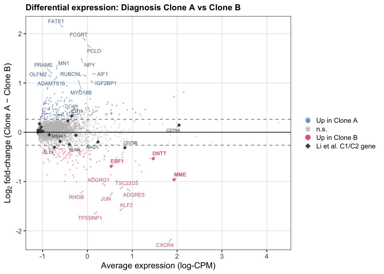
Figure panels — main figure
# Gene set enrichment — Clone A vs Clone B (camera competitive test).
# Direction="Up" = enriched in Clone A; Direction="Down" = enriched in Clone B.
# Bars show -log10(FDR); colour distinguishes enrichment direction.
# Only gene sets with FDR < 0.1 shown.

# Clean gene set names for display
clean_geneset_name <- function(x) {
  x %>%
    str_remove("^HALLMARK_|^KEGG_|^REACTOME_|^WP_|^BIOCARTA_|^SA_|^SIG_|^OSWALD_|^JAATINEN_|^RHEIN_ALL_|^DEBOSSCHER_") %>%
    str_replace_all("_", " ") %>%
    str_to_sentence() %>%
    str_replace("Bcr", "BCR") %>%
    str_replace("Mhc", "MHC") %>%
    str_replace("B cell", "B cell") %>%
    str_trunc(55, ellipsis = "…")
}

gse_ab <- cam_results %>%
  filter(contrast == "DiaAvDiaB", FDR < 0.1) %>%
  mutate(
    score    = -log10(FDR),
    label    = dplyr::case_when(
      gene_set == "Li2025 C2 (pro-B-like)" ~ "Li2025 C2 (pro-B-like)",
      gene_set == "Li2025 C1 (HSC-like)"   ~ "Li2025 C1 (HSC-like)",
      TRUE ~ clean_geneset_name(gene_set)
    ),
    enriched = ifelse(Direction == "Up", "Enriched in Clone A", "Enriched in Clone B")
  ) %>%
  arrange(score) %>%
  mutate(label = factor(label, levels = label))

ggplot(gse_ab, aes(x = score, y = label, fill = enriched, pattern = enriched)) +
  ggpattern::geom_col_pattern(
    width           = 0.7,
    pattern_colour  = "white",
    pattern_fill    = "white",
    pattern_density = 0.35,
    pattern_spacing = 0.06,
    pattern_angle   = 45
  ) +
  geom_vline(xintercept = -log10(0.05),
             linetype = "dashed", linewidth = 0.35, colour = "grey50") +
  scale_fill_manual(
    values = c("Enriched in Clone A" = "#FDAE61", "Enriched in Clone B" = "#FDAE61"),
    name   = NULL
  ) +
  ggpattern::scale_pattern_manual(
    values = c("Enriched in Clone A" = "none", "Enriched in Clone B" = "stripe"),
    name   = NULL
  ) +
  scale_x_continuous(
    name   = expression(-log[10]~FDR),
    expand = expansion(mult = c(0, 0.05))
  ) +
  labs(y = NULL) +
  theme_classic(base_size = 10) +
  theme(
    axis.text.y        = element_text(size = 8.5),
    panel.grid.major.x = element_line(colour = "grey92", linewidth = 0.3),
    legend.position    = "bottom",
    legend.text        = element_text(size = 9)
  ) -> fig4_G
fig4_G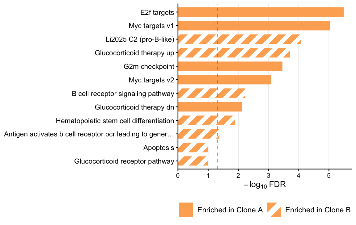
| Version | Author | Date |
|---|---|---|
| 6c36b3e | Jovana Maksimovic | 2026-07-16 |
# ETV6::RUNX1-v1 fusion detection rate per clone group.
# clone_refined is set in the clone-id chunk above.

fusion_by_clone <- seu_c1437@meta.data %>%
  as.data.frame() %>%
  filter(as.character(clone_refined) != "Normal BM") %>%
  filter(predicted_CellType_Broad %in% c("Pro-B", "Pre-B", "Early Lymphoid")) %>%
  mutate(clone_refined = factor(as.character(clone_refined),
    levels = c("Diagnosis clone A", "Diagnosis clone B", "Relapse clone"))) %>%
  group_by(clone_refined) %>%
  summarise(
    n_cells    = n(),
    n_fusion   = sum(patient_fusion == "ETV6-RUNX1-v1-fusion"),
    pct_fusion = n_fusion / n_cells * 100,
    .groups    = "drop"
  )

print(fusion_by_clone)
# A tibble: 3 × 4
clone_refined n_cells n_fusion pct_fusion
<fct> <int> <int> <dbl>
1 Diagnosis clone A 5453 1396 25.6
2 Diagnosis clone B 3856 825 21.4
3 Relapse clone 12693 4683 36.9ggplot(fusion_by_clone,
aes(x = clone_refined, y = pct_fusion,
fill = clone_refined, pattern = clone_refined)) +
ggpattern::geom_col_pattern(
width = 0.6,
pattern_colour = "white",
pattern_fill = "white",
pattern_density = 0.35,
pattern_spacing = 0.06,
pattern_angle = 45
) +
geom_text(aes(label = paste0(round(pct_fusion, 1), "%")),
vjust = -0.5, size = 3) +
scale_fill_manual(values = clone_cols[c("Diagnosis clone A",
"Diagnosis clone B",
"Relapse clone")],
guide = "none") +
ggpattern::scale_pattern_manual(
values = clone_patterns,
guide = "none"
) +
scale_x_discrete(labels = c(
"Diagnosis clone A" = "Dx clone A",
"Diagnosis clone B" = "Dx clone B",
"Relapse clone" = "Relapse"
)) +
labs(x = NULL, y = "% ETV6::RUNX1-v1 fusion-positive blasts") +
theme_classic(base_size = 11) +
theme(legend.position = "none") -> fig4_F
fig4_F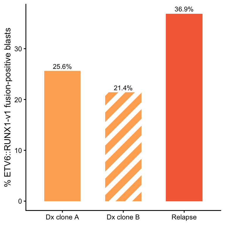
| Version | Author | Date |
|---|---|---|
| 6c36b3e | Jovana Maksimovic | 2026-07-16 |
Figure panels — supplementary figure
# Gene set enrichment for unique-to-group contrasts (CloneA_unique, CloneB_unique,
# Relapse_unique). Each contrast tests a group vs the average of the other two,
# so enrichment reflects what is distinctively up or down in that group alone.
# Colour = direction of enrichment within the named group.

# Light/dark colours per clone group
clone_cols_unique <- list(
  CloneA_unique  = c(high = "#2255AA", low = "#99BBDD"),
  CloneB_unique  = c(high = "#CC2244", low = "#EEAABB"),
  Relapse_unique = c(high = "#1A6E2E", low = "#85C49A")
)

legend_labels_unique <- list(
  CloneA_unique  = c("Higher in Clone A",  "Lower in Clone A"),
  CloneB_unique  = c("Higher in Clone B",  "Lower in Clone B"),
  Relapse_unique = c("Higher in Relapse",  "Lower in Relapse")
)

gse_unique_all <- cam_results %>%
  filter(contrast %in% names(clone_cols_unique), FDR < 0.1) %>%
  mutate(
    score = -log10(FDR),
    label = dplyr::case_when(
      gene_set == "Li2025 C2 (pro-B-like)" ~ "Li2025 C2 (pro-B-like)",
      gene_set == "Li2025 C1 (HSC-like)"   ~ "Li2025 C1 (HSC-like)",
      TRUE ~ clean_geneset_name(gene_set)
    )
  )

# Shared y-axis limit across all three panels
y_max_unique <- gse_unique_all %>%
  filter(contrast %in% names(clone_cols_unique), FDR < 0.1) %>%
  summarise(mx = max(-log10(FDR), na.rm = TRUE)) %>%
  pull(mx) * 1.08

make_unique_gse_plot <- function(ct) {
  cols   <- clone_cols_unique[[ct]]
  llabs  <- legend_labels_unique[[ct]]
  df     <- gse_unique_all %>%
    filter(contrast == ct) %>%
    mutate(
      fill_col = ifelse(Direction == "Up", cols["high"], cols["low"]),
      label    = factor(label, levels = label[order(-score)])
    )

  ggplot(df, aes(x = label, y = score, fill = fill_col)) +
    geom_col(width = 0.7) +
    geom_hline(yintercept = -log10(0.05),
               linetype = "dashed", linewidth = 0.35, colour = "grey50") +
    scale_fill_identity(
      guide  = "legend",
      labels = llabs,
      breaks = c(cols["high"], cols["low"])
    ) +
    scale_y_continuous(
      name   = expression(-log[10]~FDR),
      limits = c(0, y_max_unique),
      expand = expansion(mult = c(0, 0))
    ) +
    labs(x = NULL, fill = NULL) +
    theme_classic(base_size = 10) +
    theme(
      axis.text.x        = element_text(angle = 90, hjust = 1, vjust = 0.5, size = 7.5),
      panel.grid.major.y = element_line(colour = "grey92", linewidth = 0.3),
      legend.position      = c(1, 1),
      legend.justification = c(1, 1),
      legend.background    = element_rect(fill = "white", colour = NA),
      legend.text          = element_text(size = 8),
      plot.margin          = margin(t = 5, r = 5, b = 5, l = 5)
    )
}

p_gse_A   <- make_unique_gse_plot("CloneA_unique")
p_gse_B   <- make_unique_gse_plot("CloneB_unique")
p_gse_Rel <- make_unique_gse_plot("Relapse_unique")

p_gse_A | p_gse_B | p_gse_Rel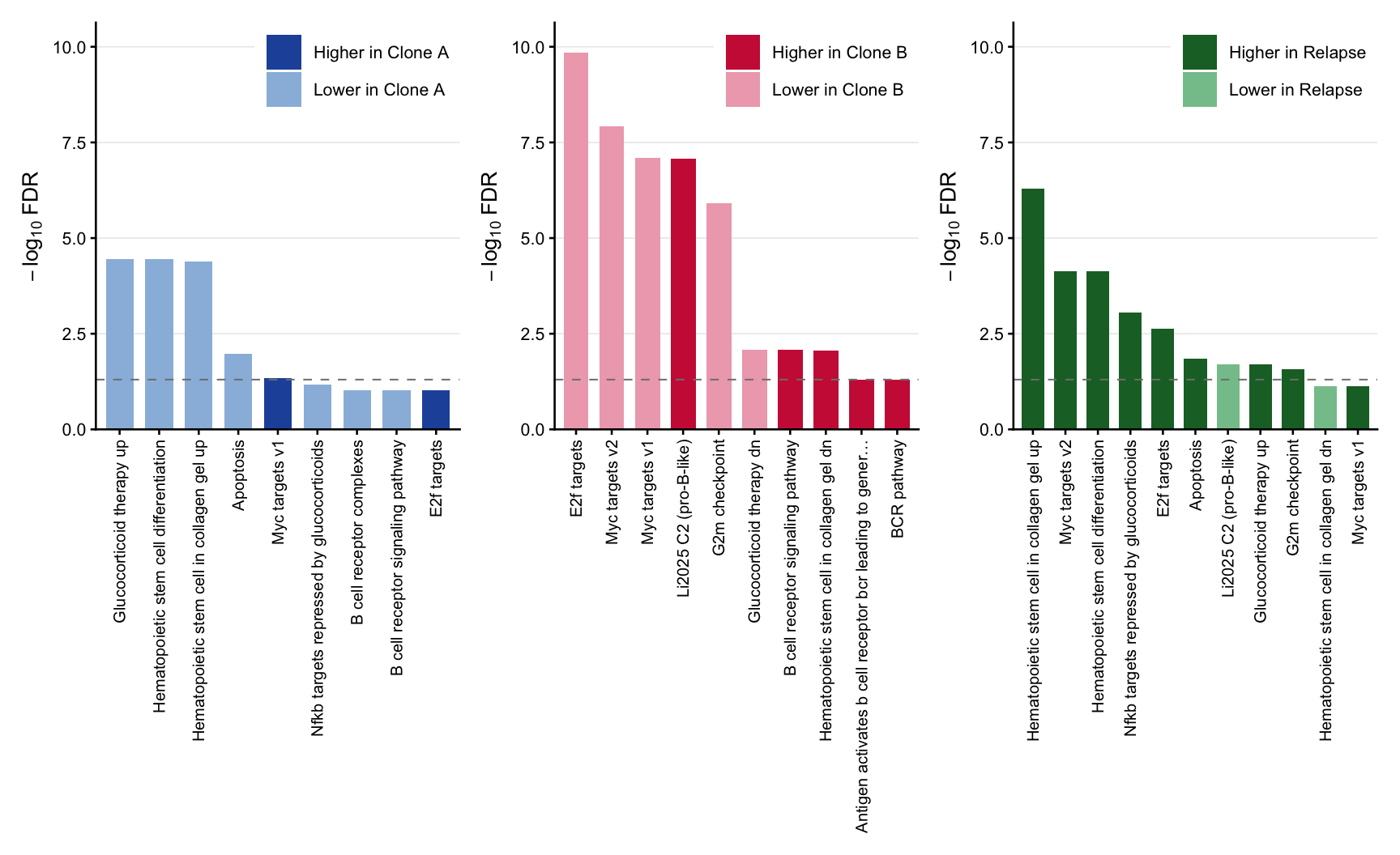
| Version | Author | Date |
|---|---|---|
| 6c36b3e | Jovana Maksimovic | 2026-07-16 |
# Unique-to-group DEG counts from balanced contrasts:
# each group vs the average of the other two (limma-trend TREAT).
# Bars show genes significantly higher (up) or lower (down) in each group
# relative to the mean of the remaining two, colour-coded by clone.

fc_thresh   <- log2(fc)
pval_thresh <- pval

unique_contrasts <- list(
  list(coef = "CloneA_unique",  group = "Diagnosis clone A"),
  list(coef = "CloneB_unique",  group = "Diagnosis clone B"),
  list(coef = "Relapse_unique", group = "Relapse clone")
)

deg_unique <- purrr::map_dfr(unique_contrasts, function(ci) {
  res <- topTreat(tr, coef = ci$coef, n = Inf)
  sig <- res[res$adj.P.Val < pval_thresh & abs(res$logFC) > fc_thresh, ]
  tibble::tibble(
    group     = ci$group,
    direction = c("Up", "Down"),
    n         = c(sum(sig$logFC > fc_thresh), -sum(sig$logFC < -fc_thresh))
  )
}) %>%
  mutate(group = factor(group, levels = c("Diagnosis clone A",
                                          "Diagnosis clone B",
                                          "Relapse clone")))

# Reuse the same blue/red/green group colours as panel D (clone_cols_unique's
# "high" shade), instead of the orange clone_cols palette used for the main
# UMAP figures, so panel C reads as part of the same group-colour scheme as D.
clone_cols_deg <- c(
  "Diagnosis clone A" = unname(clone_cols_unique$CloneA_unique["high"]),
  "Diagnosis clone B" = unname(clone_cols_unique$CloneB_unique["high"]),
  "Relapse clone"     = unname(clone_cols_unique$Relapse_unique["high"])
)

ggplot(deg_unique,
       aes(x = group, y = n,
           fill = group, alpha = direction)) +
  geom_col(width = 0.6) +
  geom_text(aes(label = abs(n),
                vjust = ifelse(n > 0, -0.4, 1.2)),
            size = 2.6) +
  geom_hline(yintercept = 0, linewidth = 0.4) +
  scale_fill_manual(values = clone_cols_deg, guide = "none") +
  scale_alpha_manual(values = c("Up" = 1, "Down" = 0.45),
                     name   = NULL,
                     labels = c("Up" = "Higher in group",
                                "Down" = "Lower in group")) +
  scale_x_discrete(labels = c(
    "Diagnosis clone A" = "Clone A",
    "Diagnosis clone B" = "Clone B",
    "Relapse clone"     = "Relapse"
  )) +
  scale_y_continuous(
    breaks = seq(-300, 300, 100),
    labels = abs,
    expand = expansion(mult = c(0.15, 0.15))
  ) +
  labs(x     = NULL,
       y     = "Unique DEGs (n)\nvs average of other two groups",
       title = "Unique DEGs per group") +
  theme_classic(base_size = 10) +
  theme(plot.title      = element_text(size = 10, face = "bold", color = "grey15",
                                       margin = margin(b = 8)),
        legend.position = "bottom",
        legend.key.size = unit(0.35, "cm"),
        legend.text     = element_text(size = 8)) -> p_deg_overlap

p_deg_overlap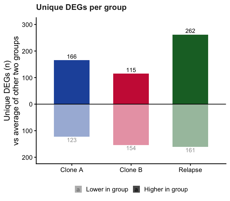
| Version | Author | Date |
|---|---|---|
| 6c36b3e | Jovana Maksimovic | 2026-07-16 |
Supplementary figure — Li et al. C1/C2 scores in C1437 clones
Single-panel figure showing the Li et al. (2025) C1 − C2 composite module score projected onto the C1437 UMAP. Both Clone A and Clone B sit predominantly in C2-like (pro-B) territory, with no clean spatial separation, motivating the direct transcriptional comparison in the main figure. Normal BM populations are labelled by broad cell type; red signal in peripheral clusters reflects genuine HSC/myeloid identity.
# ── C1 − C2 composite score UMAP with population labels --------------------- #

# Broad label lookup for Normal BM cell types
broad_label_map <- c(
  "CD8 Memory T"  = "T cell",
  "CD4 Memory T"  = "T cell",
  "Naive T"       = "T cell",
  "CD8 Effector T"= "T cell",
  "CD4 T"         = "T cell",
  "NK"            = "NK",
  "HSC MPP"       = "HSC/MPP",
  "HSC"           = "HSC/MPP",
  "MPP"           = "HSC/MPP",
  "Pro-Monocyte"  = "Monocyte",
  "Monocyte"      = "Monocyte",
  "cDC"           = "DC",
  "pDC"           = "DC",
  "B"             = "B cell",
  "Plasma Cell"   = "B cell",
  "Plasma"        = "B cell"
)

# Build centroid label data frame
umap_coords <- as.data.frame(Embeddings(seu_c1437, reduction = "umap"))
umap_coords$cell_id <- rownames(umap_coords)
umap_col1 <- colnames(umap_coords)[1]
umap_col2 <- colnames(umap_coords)[2]

meta_df <- seu_c1437@meta.data %>%
  as_tibble(rownames = "cell_id") %>%
  select(cell_id, clone_refined, predicted_CellType_Broad) %>%
  left_join(umap_coords, by = "cell_id")

# Clone A / B / Relapse centroids
clone_labels <- meta_df %>%
  filter(clone_refined != "Normal BM") %>%
  group_by(clone_refined) %>%
  summarise(x = median(.data[[umap_col1]]),
            y = median(.data[[umap_col2]]),
            .groups = "drop") %>%
  rename(label = clone_refined)

# Normal BM: recode to broad labels, merge, compute centroids (≥ 10 cells)
bm_labels <- meta_df %>%
  filter(clone_refined == "Normal BM") %>%
  mutate(broad = broad_label_map[predicted_CellType_Broad]) %>%
  filter(!is.na(broad)) %>%
  group_by(broad) %>%
  summarise(x = median(.data[[umap_col1]]),
            y = median(.data[[umap_col2]]),
            n = n(),
            .groups = "drop") %>%
  filter(n >= 10) %>%
  rename(label = "broad")

# Capitalise "Clone" in clone labels for display
clone_labels <- clone_labels %>%
  mutate(label = str_replace(label, "clone", "Clone"))

all_labels <- bind_rows(clone_labels, bm_labels)

# Build plot manually to allow per-group point sizes
plot_df <- meta_df %>%
  left_join(
    seu_c1437@meta.data %>%
      as_tibble(rownames = "cell_id") %>%
      select(cell_id, Li2025_C1vsC2),
    by = "cell_id"
  ) %>%
  mutate(pt_size = ifelse(clone_refined == "Normal BM", 0.3, 0.5)) %>%
  arrange(Li2025_C1vsC2)   # order = TRUE equivalent: high values plotted last

fig_supp <- ggplot(
  plot_df,
  aes(x = .data[[umap_col1]], y = .data[[umap_col2]], colour = Li2025_C1vsC2)
) +
  geom_point(aes(size = pt_size), alpha = 0.8) +
  scale_size_identity() +
  scale_colour_distiller(
    palette   = "RdBu",
    direction = -1,
    limits    = c(-0.6, 0.6),
    oob       = scales::squish,
    name      = "C1 − C2"
  ) +
  # Clone labels — larger, dark
  ggrepel::geom_text_repel(
    data          = clone_labels,
    aes(x = x, y = y, label = label),
    inherit.aes   = FALSE,
    size          = 3.5,
    colour        = "grey10",
    box.padding   = 0.4,
    point.padding = 0.2,
    max.overlaps  = 20,
    segment.size  = 0.3,
    segment.colour = "grey40"
  ) +
  # Normal BM labels — smaller, lighter
  ggrepel::geom_text_repel(
    data          = bm_labels,
    aes(x = x, y = y, label = label),
    inherit.aes   = FALSE,
    size          = 2.8,
    colour        = "grey50",
    box.padding   = 0.4,
    point.padding = 0.2,
    max.overlaps  = 20,
    segment.size  = 0.25,
    segment.colour = "grey65"
  ) +
  labs(x = umap_col1, y = umap_col2) +
  labs(
    title  = "C1 − C2 composite score",
    colour = "C1 − C2"
  ) +
  theme_pub() +
  theme(
    legend.position  = "bottom",
    legend.direction = "horizontal",
    legend.key.width = unit(1.2, "cm"),
    legend.key.height = unit(0.3, "cm"),
    legend.text      = element_text(size = 8)
  )

# ── Save PNG ----------------------------------------------------------------- #
out_dir <- here("output")
if (!dir.exists(out_dir)) dir.create(out_dir, recursive = TRUE)

ggsave(
  filename = file.path(out_dir, "supp_figure_c1437_li2025_scores.png"),
  plot     = fig_supp,
  width    = 7,
  height   = 6,
  dpi      = 300,
  bg       = "white"
)

fig_supp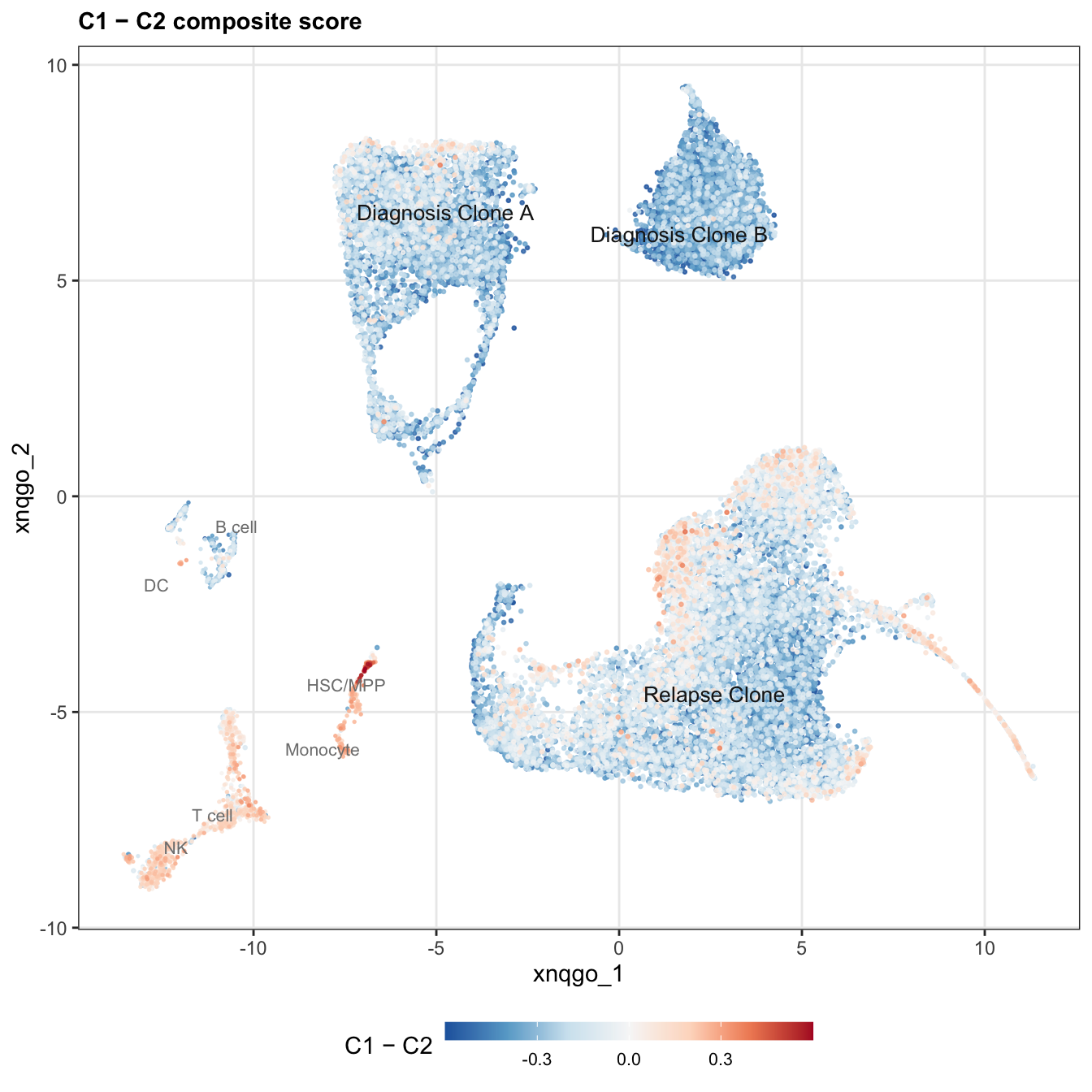
Supplementary figure: Li et al. C1/C2 composite score on C1437 UMAP.
Assemble full patchwork (Supplementary Figure 5)
Four-panel publication assembly: (A) C1 − C2 composite score UMAP
(fig_supp), (B) differential expression MA plot for
Diagnosis Clone A vs Clone B (p_ma_inline), (C) unique-DEG
bar chart (p_deg_overlap), (D) gene set enrichment for
Clone A / Clone B / Relapse unique contrasts (p_gse_A,
p_gse_B, p_gse_Rel, combined side by side).
Tagging follows the same approach as
B-ALL_exp2_quality_control.Rmd’s Supplementary Figure 4
assembly: panel D is itself three separate ggplots combined with
|, so wrap_elements() converts each conceptual
panel — including the combined D row — into a single opaque patch before
plot_annotation() assigns tags, giving exactly four tags
(A–D) rather than six. Panel C is narrower than panel D in the layout
since D holds three sub-panels against C’s one.
tag_theme <- theme(plot.tag = element_text(size = 18, face = "bold"))

pA <- fig_supp
pB <- p_ma_inline
pC <- p_deg_overlap

# Panel D combines three separate GSEA plots; give the row a single shared
# title the same way Supp Fig 4's nested violin stack is titled in
# B-ALL_exp2_quality_control.Rmd, so it reads as one labelled panel.
pD <- (p_gse_A | p_gse_B | p_gse_Rel) +
  plot_annotation(title = "Gene set enrichment by group",
                  theme = theme(plot.title = element_text(
                    size = 10, face = "bold", color = "grey15",
                    margin = margin(b = 8))))

pA_tagged <- wrap_elements(pA) + tag_theme
pB_tagged <- wrap_elements(pB) + tag_theme
pC_tagged <- wrap_elements(pC) + tag_theme
pD_tagged <- wrap_elements(pD) + tag_theme

supp5_design <- "
AABB
CDDD
"

full_patchwork <- pA_tagged + pB_tagged + pC_tagged + pD_tagged +
  plot_layout(design = supp5_design, heights = c(1.3, 1)) +
  plot_annotation(tag_levels = "A")

full_patchwork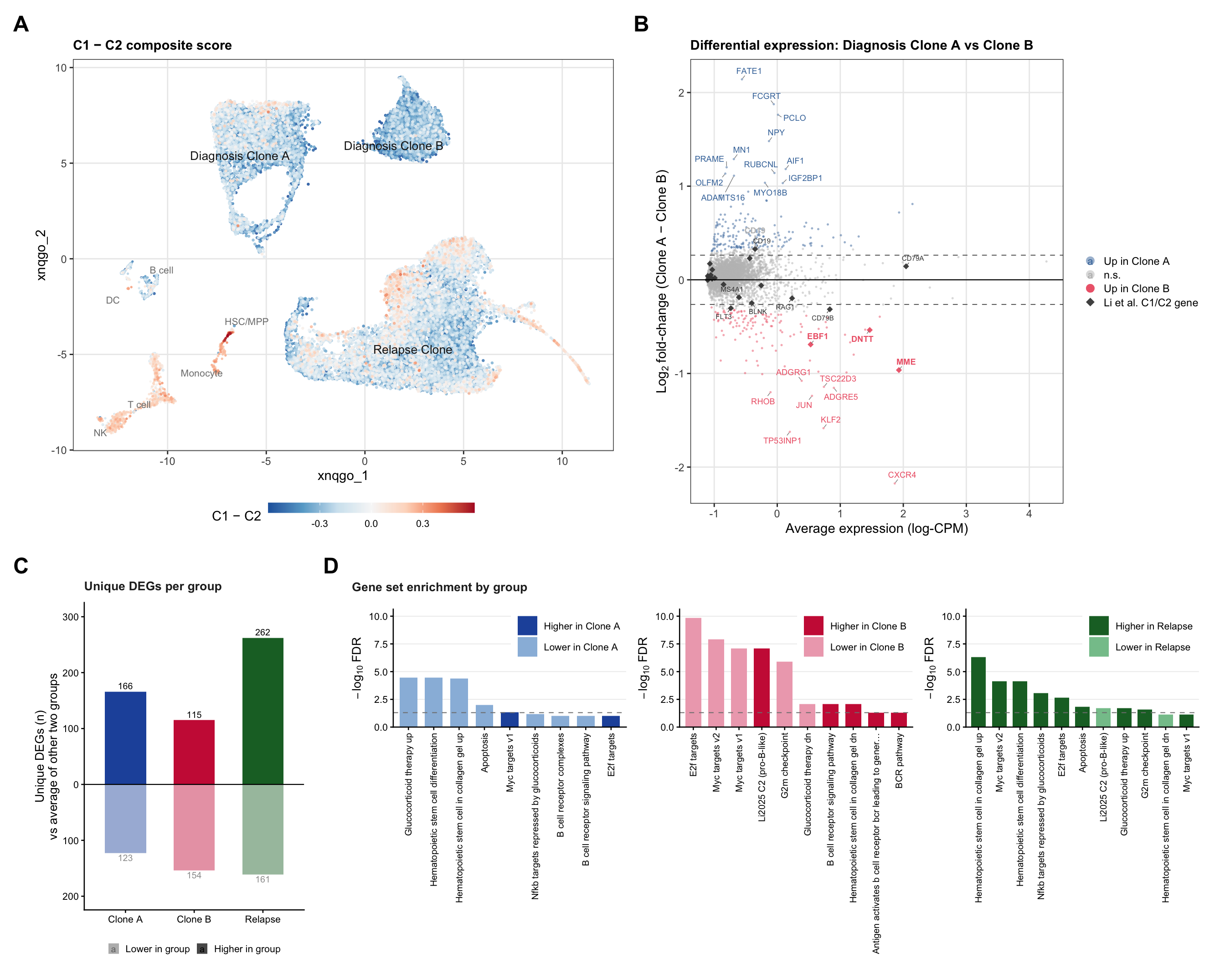
ggsave(here("output", "supp_fig5_c1437_patchwork.pdf"), full_patchwork,
      width = 12, height = 9)
ggsave(here("output", "supp_fig5_c1437_patchwork.png"), full_patchwork,
      width = 12, height = 9, dpi = 300)
Session info
sessionInfo()R version 4.4.1 (2024-06-14)
Platform: aarch64-apple-darwin20
Running under: macOS 15.7.9
Matrix products: default
BLAS: /Library/Frameworks/R.framework/Versions/4.4-arm64/Resources/lib/libRblas.0.dylib
LAPACK: /Library/Frameworks/R.framework/Versions/4.4-arm64/Resources/lib/libRlapack.dylib; LAPACK version 3.12.0
locale:
[1] en_US.UTF-8/en_US.UTF-8/en_US.UTF-8/C/en_US.UTF-8/en_US.UTF-8
time zone: Australia/Melbourne
tzcode source: internal
attached base packages:
[1] stats4 stats graphics grDevices datasets utils methods
[8] base
other attached packages:
[1] future_1.49.0 msigdbr_25.1.1
[3] speckle_1.6.0 edgeR_4.4.2
[5] limma_3.62.2 ggpattern_1.3.1
[7] clustree_0.5.1 ggraph_2.2.1
[9] scales_1.4.0 fs_1.6.6
[11] glue_1.8.0 here_1.0.1
[13] ggrepel_0.9.6 patchwork_1.3.0
[15] lubridate_1.9.4 forcats_1.0.0
[17] stringr_1.6.0 dplyr_1.1.4
[19] purrr_1.0.4 readr_2.1.5
[21] tidyr_1.3.1 tibble_3.2.1
[23] ggplot2_4.0.2 tidyverse_2.0.0
[25] scran_1.34.0 scuttle_1.16.0
[27] SingleCellExperiment_1.28.1 SummarizedExperiment_1.36.0
[29] Biobase_2.66.0 GenomicRanges_1.58.0
[31] GenomeInfoDb_1.42.3 IRanges_2.40.1
[33] S4Vectors_0.44.0 BiocGenerics_0.52.0
[35] MatrixGenerics_1.18.1 matrixStats_1.5.0
[37] Seurat_5.3.0 SeuratObject_5.1.0
[39] sp_2.2-0 workflowr_1.7.1
loaded via a namespace (and not attached):
[1] spatstat.sparse_3.1-0 sf_1.1-1
[3] httr_1.4.7 RColorBrewer_1.1-3
[5] tools_4.4.1 sctransform_0.4.2
[7] backports_1.5.0 utf8_1.2.5
[9] R6_2.6.1 lazyeval_0.2.2
[11] uwot_0.2.3 withr_3.0.2
[13] gridExtra_2.3 progressr_0.15.1
[15] textshaping_1.0.1 cli_3.6.5
[17] spatstat.explore_3.4-3 fastDummies_1.7.5
[19] labeling_0.4.3 sass_0.4.10
[21] S7_0.2.0 spatstat.data_3.1-6
[23] proxy_0.4-27 ggridges_0.5.6
[25] pbapply_1.7-4 systemfonts_1.2.3
[27] parallelly_1.45.0 rstudioapi_0.17.1
[29] generics_0.1.4 ica_1.0-3
[31] spatstat.random_3.4-1 Matrix_1.7-0
[33] abind_1.4-8 lifecycle_1.0.4
[35] whisker_0.4.1 yaml_2.3.10
[37] SparseArray_1.6.2 Rtsne_0.17
[39] glmGamPoi_1.18.0 grid_4.4.1
[41] promises_1.3.3 dqrng_0.4.1
[43] crayon_1.5.3 miniUI_0.1.2
[45] lattice_0.22-6 beachmat_2.22.0
[47] cowplot_1.1.3 pillar_1.10.2
[49] knitr_1.50 metapod_1.14.0
[51] future.apply_1.11.3 codetools_0.2-20
[53] getPass_0.2-4 leidenbase_0.1.35
[55] spatstat.univar_3.1-3 data.table_1.18.2.1
[57] vctrs_0.6.5 png_0.1-8
[59] spam_2.11-1 gtable_0.3.6
[61] assertthat_0.2.1 cachem_1.1.0
[63] xfun_0.56 S4Arrays_1.6.0
[65] mime_0.13 tidygraph_1.3.1
[67] survival_3.6-4 units_1.0-1
[69] statmod_1.5.0 bluster_1.16.0
[71] fitdistrplus_1.2-2 ROCR_1.0-11
[73] nlme_3.1-164 RcppAnnoy_0.0.22
[75] rprojroot_2.0.4 bslib_0.9.0
[77] irlba_2.3.5.1 KernSmooth_2.23-24
[79] DBI_1.2.3 colorspace_2.1-1
[81] tidyselect_1.2.1 processx_3.8.6
[83] compiler_4.4.1 curl_6.2.3
[85] git2r_0.36.2 BiocNeighbors_2.0.1
[87] DelayedArray_0.32.0 plotly_4.10.4
[89] checkmate_2.3.2 classInt_0.4-11
[91] lmtest_0.9-40 callr_3.7.6
[93] digest_0.6.37 goftest_1.2-3
[95] spatstat.utils_3.1-4 rmarkdown_2.29
[97] XVector_0.46.0 htmltools_0.5.8.1
[99] pkgconfig_2.0.3 sparseMatrixStats_1.18.0
[101] fastmap_1.2.0 rlang_1.1.6
[103] htmlwidgets_1.6.4 UCSC.utils_1.2.0
[105] shiny_1.10.0 DelayedMatrixStats_1.28.1
[107] farver_2.1.2 jquerylib_0.1.4
[109] zoo_1.8-14 jsonlite_2.0.0
[111] BiocParallel_1.40.2 BiocSingular_1.22.0
[113] magrittr_2.0.3 GenomeInfoDbData_1.2.13
[115] dotCall64_1.2 Rcpp_1.1.1-1.1
[117] babelgene_22.9 viridis_0.6.5
[119] reticulate_1.42.0 stringi_1.8.7
[121] zlibbioc_1.52.0 MASS_7.3-60.2
[123] plyr_1.8.9 parallel_4.4.1
[125] listenv_0.9.1 deldir_2.0-4
[127] graphlayouts_1.2.2 splines_4.4.1
[129] tensor_1.5 hms_1.1.3
[131] locfit_1.5-9.12 ps_1.9.1
[133] igraph_2.1.4 spatstat.geom_3.4-1
[135] RcppHNSW_0.6.0 reshape2_1.4.4
[137] ScaledMatrix_1.14.0 evaluate_1.0.3
[139] renv_1.1.4 BiocManager_1.30.27
[141] tzdb_0.5.0 tweenr_2.0.3
[143] httpuv_1.6.16 RANN_2.6.2
[145] polyclip_1.10-7 scattermore_1.2
[147] ggforce_0.4.2 rsvd_1.0.5
[149] xtable_1.8-4 e1071_1.7-16
[151] RSpectra_0.16-2 later_1.4.2
[153] ragg_1.4.0 class_7.3-22
[155] viridisLite_0.4.2 memoise_2.0.1
[157] gridpattern_1.4.2 cluster_2.1.6
[159] timechange_0.3.0 globals_0.18.0
sessionInfo()R version 4.4.1 (2024-06-14)
Platform: aarch64-apple-darwin20
Running under: macOS 15.7.9
Matrix products: default
BLAS: /Library/Frameworks/R.framework/Versions/4.4-arm64/Resources/lib/libRblas.0.dylib
LAPACK: /Library/Frameworks/R.framework/Versions/4.4-arm64/Resources/lib/libRlapack.dylib; LAPACK version 3.12.0
locale:
[1] en_US.UTF-8/en_US.UTF-8/en_US.UTF-8/C/en_US.UTF-8/en_US.UTF-8
time zone: Australia/Melbourne
tzcode source: internal
attached base packages:
[1] stats4 stats graphics grDevices datasets utils methods
[8] base
other attached packages:
[1] future_1.49.0 msigdbr_25.1.1
[3] speckle_1.6.0 edgeR_4.4.2
[5] limma_3.62.2 ggpattern_1.3.1
[7] clustree_0.5.1 ggraph_2.2.1
[9] scales_1.4.0 fs_1.6.6
[11] glue_1.8.0 here_1.0.1
[13] ggrepel_0.9.6 patchwork_1.3.0
[15] lubridate_1.9.4 forcats_1.0.0
[17] stringr_1.6.0 dplyr_1.1.4
[19] purrr_1.0.4 readr_2.1.5
[21] tidyr_1.3.1 tibble_3.2.1
[23] ggplot2_4.0.2 tidyverse_2.0.0
[25] scran_1.34.0 scuttle_1.16.0
[27] SingleCellExperiment_1.28.1 SummarizedExperiment_1.36.0
[29] Biobase_2.66.0 GenomicRanges_1.58.0
[31] GenomeInfoDb_1.42.3 IRanges_2.40.1
[33] S4Vectors_0.44.0 BiocGenerics_0.52.0
[35] MatrixGenerics_1.18.1 matrixStats_1.5.0
[37] Seurat_5.3.0 SeuratObject_5.1.0
[39] sp_2.2-0 workflowr_1.7.1
loaded via a namespace (and not attached):
[1] spatstat.sparse_3.1-0 sf_1.1-1
[3] httr_1.4.7 RColorBrewer_1.1-3
[5] tools_4.4.1 sctransform_0.4.2
[7] backports_1.5.0 utf8_1.2.5
[9] R6_2.6.1 lazyeval_0.2.2
[11] uwot_0.2.3 withr_3.0.2
[13] gridExtra_2.3 progressr_0.15.1
[15] textshaping_1.0.1 cli_3.6.5
[17] spatstat.explore_3.4-3 fastDummies_1.7.5
[19] labeling_0.4.3 sass_0.4.10
[21] S7_0.2.0 spatstat.data_3.1-6
[23] proxy_0.4-27 ggridges_0.5.6
[25] pbapply_1.7-4 systemfonts_1.2.3
[27] parallelly_1.45.0 rstudioapi_0.17.1
[29] generics_0.1.4 ica_1.0-3
[31] spatstat.random_3.4-1 Matrix_1.7-0
[33] abind_1.4-8 lifecycle_1.0.4
[35] whisker_0.4.1 yaml_2.3.10
[37] SparseArray_1.6.2 Rtsne_0.17
[39] glmGamPoi_1.18.0 grid_4.4.1
[41] promises_1.3.3 dqrng_0.4.1
[43] crayon_1.5.3 miniUI_0.1.2
[45] lattice_0.22-6 beachmat_2.22.0
[47] cowplot_1.1.3 pillar_1.10.2
[49] knitr_1.50 metapod_1.14.0
[51] future.apply_1.11.3 codetools_0.2-20
[53] getPass_0.2-4 leidenbase_0.1.35
[55] spatstat.univar_3.1-3 data.table_1.18.2.1
[57] vctrs_0.6.5 png_0.1-8
[59] spam_2.11-1 gtable_0.3.6
[61] assertthat_0.2.1 cachem_1.1.0
[63] xfun_0.56 S4Arrays_1.6.0
[65] mime_0.13 tidygraph_1.3.1
[67] survival_3.6-4 units_1.0-1
[69] statmod_1.5.0 bluster_1.16.0
[71] fitdistrplus_1.2-2 ROCR_1.0-11
[73] nlme_3.1-164 RcppAnnoy_0.0.22
[75] rprojroot_2.0.4 bslib_0.9.0
[77] irlba_2.3.5.1 KernSmooth_2.23-24
[79] DBI_1.2.3 colorspace_2.1-1
[81] tidyselect_1.2.1 processx_3.8.6
[83] compiler_4.4.1 curl_6.2.3
[85] git2r_0.36.2 BiocNeighbors_2.0.1
[87] DelayedArray_0.32.0 plotly_4.10.4
[89] checkmate_2.3.2 classInt_0.4-11
[91] lmtest_0.9-40 callr_3.7.6
[93] digest_0.6.37 goftest_1.2-3
[95] spatstat.utils_3.1-4 rmarkdown_2.29
[97] XVector_0.46.0 htmltools_0.5.8.1
[99] pkgconfig_2.0.3 sparseMatrixStats_1.18.0
[101] fastmap_1.2.0 rlang_1.1.6
[103] htmlwidgets_1.6.4 UCSC.utils_1.2.0
[105] shiny_1.10.0 DelayedMatrixStats_1.28.1
[107] farver_2.1.2 jquerylib_0.1.4
[109] zoo_1.8-14 jsonlite_2.0.0
[111] BiocParallel_1.40.2 BiocSingular_1.22.0
[113] magrittr_2.0.3 GenomeInfoDbData_1.2.13
[115] dotCall64_1.2 Rcpp_1.1.1-1.1
[117] babelgene_22.9 viridis_0.6.5
[119] reticulate_1.42.0 stringi_1.8.7
[121] zlibbioc_1.52.0 MASS_7.3-60.2
[123] plyr_1.8.9 parallel_4.4.1
[125] listenv_0.9.1 deldir_2.0-4
[127] graphlayouts_1.2.2 splines_4.4.1
[129] tensor_1.5 hms_1.1.3
[131] locfit_1.5-9.12 ps_1.9.1
[133] igraph_2.1.4 spatstat.geom_3.4-1
[135] RcppHNSW_0.6.0 reshape2_1.4.4
[137] ScaledMatrix_1.14.0 evaluate_1.0.3
[139] renv_1.1.4 BiocManager_1.30.27
[141] tzdb_0.5.0 tweenr_2.0.3
[143] httpuv_1.6.16 RANN_2.6.2
[145] polyclip_1.10-7 scattermore_1.2
[147] ggforce_0.4.2 rsvd_1.0.5
[149] xtable_1.8-4 e1071_1.7-16
[151] RSpectra_0.16-2 later_1.4.2
[153] ragg_1.4.0 class_7.3-22
[155] viridisLite_0.4.2 memoise_2.0.1
[157] gridpattern_1.4.2 cluster_2.1.6
[159] timechange_0.3.0 globals_0.18.0