B-ALL Experiment 2: Per-sample Clustering

Per-sample SCTransform/Leiden clustering, C1437 clone annotation, and C369 MRD marker analysis

workflowr

• Summary
• Checks
• Past versions

Last updated: 2026-07-16

Checks: 7 0

Knit directory: flex-fusion-probes/

This reproducible R Markdown analysis was created with workflowr (version 1.7.1). The Checks tab describes the reproducibility checks that were applied when the results were created. The Past versions tab lists the development history.

---

R Markdown file: up-to-date

Great! Since the R Markdown file has been committed to the Git repository, you know the exact version of the code that produced these results.

Environment: empty

Great job! The global environment was empty. Objects defined in the global environment can affect the analysis in your R Markdown file in unknown ways. For reproduciblity it’s best to always run the code in an empty environment.

Seed: set.seed(20240925)

The command set.seed(20240925) was run prior to running the code in the R Markdown file. Setting a seed ensures that any results that rely on randomness, e.g. subsampling or permutations, are reproducible.

Session information: recorded

Great job! Recording the operating system, R version, and package versions is critical for reproducibility.

Cache: none

Nice! There were no cached chunks for this analysis, so you can be confident that you successfully produced the results during this run.

File paths: relative

Great job! Using relative paths to the files within your workflowr project makes it easier to run your code on other machines.

Repository version: 510ab74

Great! You are using Git for version control. Tracking code development and connecting the code version to the results is critical for reproducibility.

The results in this page were generated with repository version 510ab74. See the Past versions tab to see a history of the changes made to the R Markdown and HTML files.

Note that you need to be careful to ensure that all relevant files for the analysis have been committed to Git prior to generating the results (you can use wflow_publish or wflow_git_commit). workflowr only checks the R Markdown file, but you know if there are other scripts or data files that it depends on. Below is the status of the Git repository when the results were generated:

Ignored files:
    Ignored:    .DS_Store
    Ignored:    .Rhistory
    Ignored:    .Rproj.user/
    Ignored:    analysis/.gitignore
    Ignored:    analysis/figure/
    Ignored:    analysis/obsolete/B-ALL_nonblast_fusion_analysis_cache/
    Ignored:    analysis/projectionFigures/
    Ignored:    code/files/
    Ignored:    data/.DS_Store
    Ignored:    data/BoneMarrowMap/
    Ignored:    data/BoneMarrowMapBoneMarrowMap_SymphonyReference.rds
    Ignored:    data/BoneMarrowMapBoneMarrowMap_uwot_model.uwot
    Ignored:    data/CAPTURE-1-POOL-FLEX/
    Ignored:    data/CAPTURE-2-POOL-FLEX/
    Ignored:    data/Pool-240917-FLEX/
    Ignored:    data/RDS/
    Ignored:    data/Run_1_and_Run_2/
    Ignored:    data/Run_2/
    Ignored:    logs/
    Ignored:    output/
    Ignored:    projectionFigures/
    Ignored:    renv/library/
    Ignored:    renv/staging/

Untracked files:
    Untracked:  CLAUDE.md
    Untracked:  analysis/B-ALL_exp2_c1437_clone_analysis.Rmd
    Untracked:  analysis/B-ALL_exp2_c369_mrd_analysis.Rmd
    Untracked:  analysis/B-ALL_exp2_fig4_assembly.Rmd
    Untracked:  analysis/B-ALL_exp2_joint_clustering.Rmd
    Untracked:  analysis/B-ALL_exp2_nonblast_fusion_analysis.Rmd
    Untracked:  data/sample_information_flex_experiment_2_table.csv
    Untracked:  poster.pptx

Unstaged changes:
    Deleted:    analysis/B-ALL_exp2_background.Rmd
    Deleted:    analysis/B-ALL_exp2_c1437_li2025_clone_analysis.Rmd
    Deleted:    analysis/B-ALL_nonblast_fusion_analysis.Rmd
    Modified:   analysis/index.Rmd
    Modified:   render_all.sh

Note that any generated files, e.g. HTML, png, CSS, etc., are not included in this status report because it is ok for generated content to have uncommitted changes.

---

These are the previous versions of the repository in which changes were made to the R Markdown (analysis/B-ALL_exp2_clustering.Rmd) and HTML (docs/B-ALL_exp2_clustering.html) files. If you’ve configured a remote Git repository (see ?wflow_git_remote), click on the hyperlinks in the table below to view the files as they were in that past version.

File	Version	Author	Date	Message
Rmd	510ab74	Jovana Maksimovic	2026-07-16	wflow_publish("analysis/B-ALL_exp2_clustering.Rmd")
html	abab370	Jovana Maksimovic	2026-05-19	Build site.
Rmd	5481825	Jovana Maksimovic	2026-05-19	Update figure labels, add C369 heading, comment out exp1 DE section, minor point size
html	74aa8d8	Jovana Maksimovic	2026-05-19	Build site.
Rmd	700df84	Jovana Maksimovic	2026-05-19	MRD dot plot: n labels, fusion -ve label, remove reclassify-ambient chunk and Poisson
html	a8def9a	Jovana Maksimovic	2026-05-18	Build site.
Rmd	08f1e2b	Jovana Maksimovic	2026-05-18	Update index and exp1/exp2 notebooks
html	1b5bb97	Jovana Maksimovic	2026-05-11	Build site.
Rmd	af3bc31	Jovana Maksimovic	2026-05-11	Re-run all notebooks with updated RDS naming scheme
Rmd	1f3159b	Jovana Maksimovic	2026-05-08	Rename RDS checkpoints to systematic naming scheme
Rmd	71c5f99	Jovana Maksimovic	2026-05-08	docs: add getting_started page; fix myeloid_types error; move exploratory notebooks to obsolete
Rmd	1578018	Jovana Maksimovic	2026-05-08	docs: add prose, standardise headings and figure labels across all 10 B-ALL notebooks
Rmd	1a33400	Jovana Maksimovic	2026-05-08	B-ALL cleanup: fix index links, stray library() calls, add chunk labels
Rmd	1724beb	Jovana Maksimovic	2026-05-08	Standardise YAML headers and chunk names across all notebooks; merge utility_functions into utilities.R
Rmd	10d2f5e	Jovana Maksimovic	2026-05-08	Rename analysis notebooks to new naming scheme

---

This notebook performs per-sample clustering of all eight Experiment 2 B-ALL samples, examines fusion transcript detection in the context of cell type and cell cycle, and produces the following publication figures: a lineage marker dot plot across blast populations (Figure 4D), a bar chart of the percentage of ETV6::RUNX1 fusion-positive cells per sample (Figure 4E), the C369 BoneMarrowMap UMAP across timepoints (Figure 4I), and a B-precursor marker dot plot for C369 MRD cell groups (Figure 4J). An exploratory C1437 clone overview is also included here; the canonical publication C1437 figures (4F–4H) are produced in B-ALL_exp2_c1437_clone_analysis.Rmd.

Load data

file <- here("data", "RDS", "ball_exp2_annotated.seu.rds")
seu <- readRDS(file)

All cells from the eight patient samples are normalised together and projected into a shared UMAP embedding for an initial overview of sample composition and cell type distribution.

seu <- NormalizeData(seu)
seu <- FindVariableFeatures(seu, selection.method = "vst", 
                                  nfeatures = 3000, verbose = FALSE)
seu <- ScaleData(seu)
seu <- RunPCA(seu, verbose = FALSE, npcs = 30)
seu <- RunUMAP(seu, dims = 1:30, reduction = "pca")

Plot UMAP labelled by sample and reference annotations.

DimPlot(seu, reduction = "umap", group.by = "patient_timepoint", 
        label = FALSE, repel = TRUE, label.size = 2.5, ) +
  scale_color_manual(values = RColorBrewer::brewer.pal(n = 8, "Dark2")) +
  guides(colour = guide_legend(ncol = 3,
                               override.aes = list(size = 3))) +
  theme(legend.position = "bottom")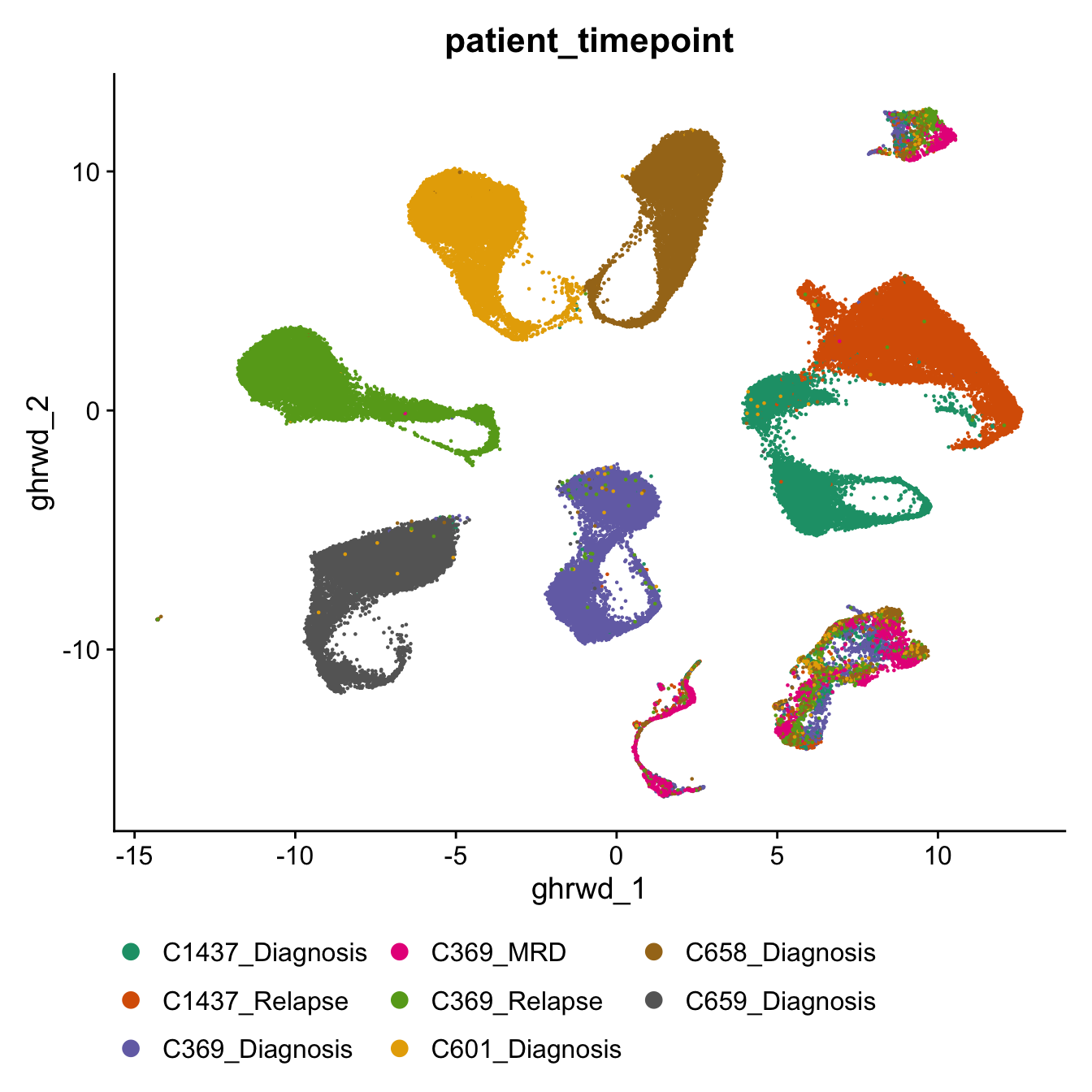

Past versions of plot-umap-overview-1.png

Version	Author	Date
1b5bb97	Jovana Maksimovic	2026-05-11

DimPlot(seu, reduction = "umap", group.by = "PPID", 
        label = FALSE, repel = TRUE, label.size = 2.5, ) +
  scale_color_manual(values = RColorBrewer::brewer.pal(n = 8, "Set2")) +
  guides(colour = guide_legend(ncol = 3,
                               override.aes = list(size = 3))) +
  theme(legend.position = "bottom")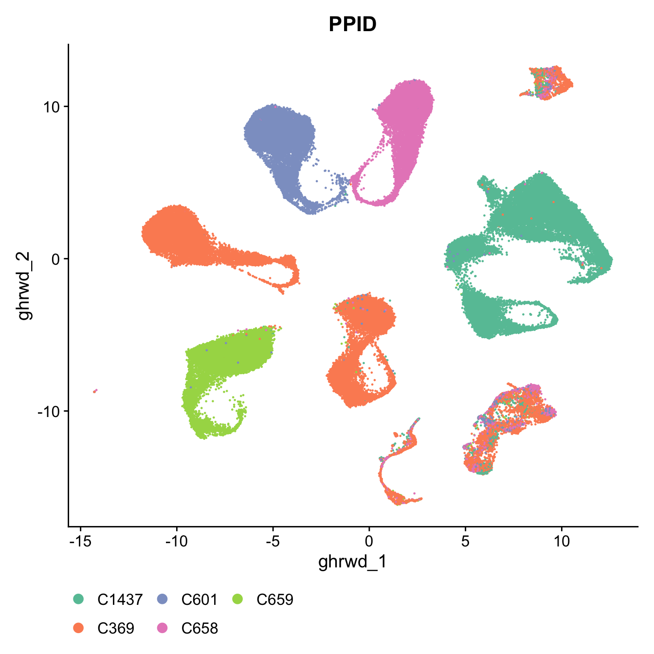

Past versions of plot-umap-overview-2.png

Version	Author	Date
1b5bb97	Jovana Maksimovic	2026-05-11

DimPlot(seu, reduction = "umap", group.by = "predicted_CellType_Broad") +
  paletteer::scale_color_paletteer_d("pals::glasbey") +
  guides(colour = guide_legend(ncol = 3,
                               override.aes = list(size = 3))) +
  theme(legend.position = "bottom")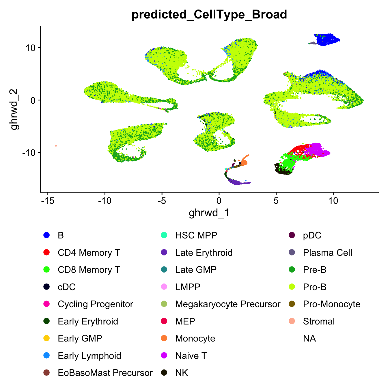 

Past versions of plot-umap-overview-3.png

Version	Author	Date
1b5bb97	Jovana Maksimovic	2026-05-11

DimPlot(seu, reduction = "umap", label = FALSE, repel = TRUE,
          label.size = 2.5, group.by = "patient_timepoint", 
          cells.highlight = which(seu$patient_fusion != "not-detected"),
          sizes.highlight = 0.1) +
    NoLegend()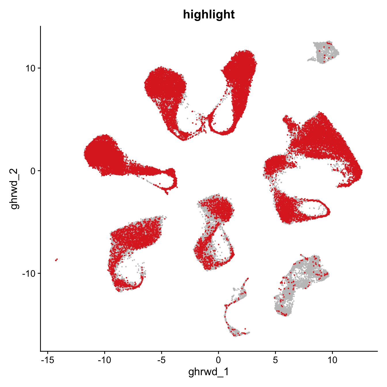 

Past versions of plot-umap-overview-4.png

Version	Author	Date
1b5bb97	Jovana Maksimovic	2026-05-11

DimPlot(seu, reduction = "umap", label = TRUE, repel = TRUE,
          label.size = 2.5, group.by = "batch")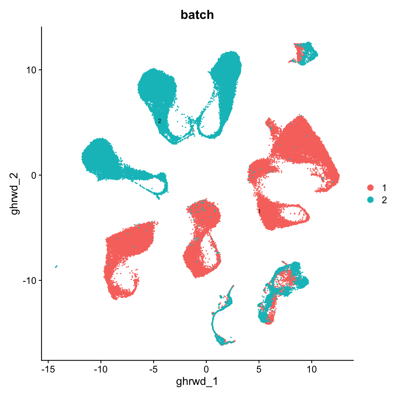 

Past versions of plot-umap-overview-5.png

Version	Author	Date
1b5bb97	Jovana Maksimovic	2026-05-11

DimPlot(seu, reduction = "umap", label = TRUE, repel = TRUE,
          label.size = 2.5, group.by = "status")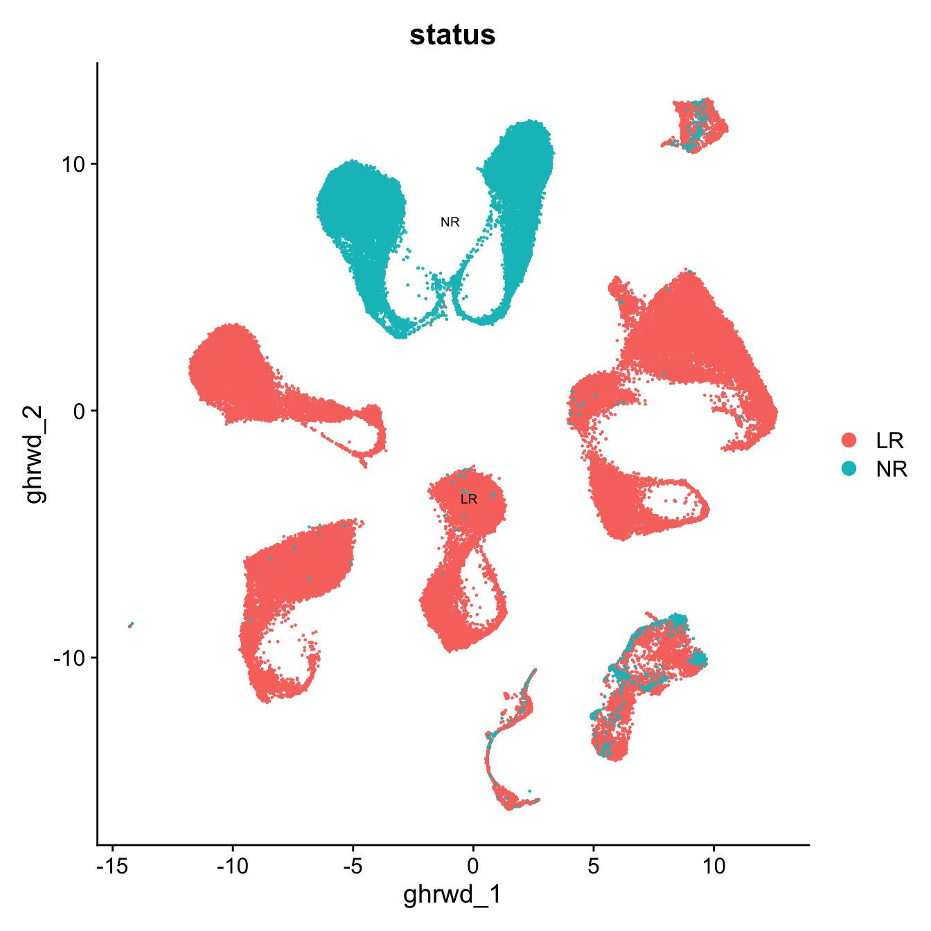

Past versions of plot-umap-overview-6.png

Version	Author	Date
1b5bb97	Jovana Maksimovic	2026-05-11

# Calculate median proportion of fusion-positive cells per sample
median_prop <- seu@meta.data %>%
  group_by(patient_timepoint) %>%
  summarise(prop_fusion = sum(fusion_detected)/n()) %>%
  summarise(median_prop = median(prop_fusion, na.rm = TRUE)) %>%
  pull(median_prop)

seu@meta.data %>%
    ggplot() +
    geom_bar(mapping = aes(x = patient_timepoint, 
                           fill = fusion_detected), 
             position = 'fill') + 
  geom_hline(yintercept = median_prop, linetype = "dashed") +
  theme_bw() +
    theme(axis.text.x = element_text(angle = 90, hjust = 1, vjust = 0.5)) +
    labs(x = "Sample",
         y = "Proportion",
         fill = "Fusion detected")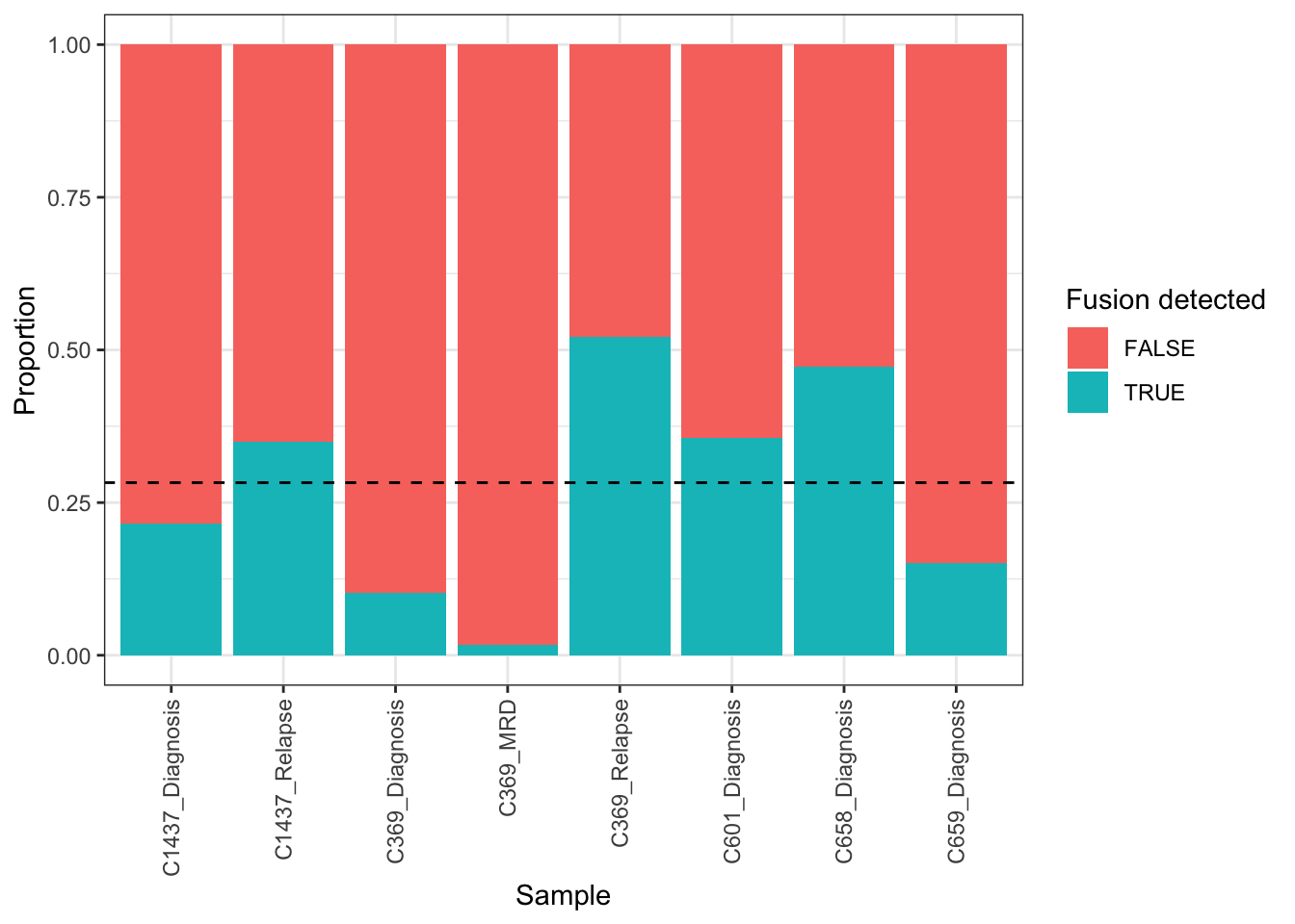

Past versions of fusion-proportion-1.png

Version	Author	Date
1b5bb97	Jovana Maksimovic	2026-05-11

seu@meta.data %>%
  dplyr::filter(fusion_detected) %>%
  ggplot(aes(x = patient_timepoint, fill = PPID)) + 
  geom_bar() +
  theme_bw() +
    theme(axis.text.x = element_blank(),
          axis.title.x = element_blank(),
          axis.ticks.x = element_blank(),
          legend.justification = "left") +
  labs(x = "Sample", y = "No. cells",
       fill = "Patient") +
  geom_text(
    stat = "count",
    aes(label = after_stat(count)),
    vjust = -0.3,
    size = 3
  ) -> p1

seu@meta.data %>%
  dplyr::filter(fusion_detected) %>%
    ggplot() +
    geom_bar(mapping = aes(x = patient_timepoint, 
                           fill = predicted_CellType_Broad), 
             position = 'fill') + 
  theme_bw() +
    theme(axis.text.x = element_text(angle = 90, hjust = 1, vjust = 0.5)) +
    labs(x = "Sample",
         y = "Proportion",
         fill = "Bone marrow reference cell type") + 
  paletteer::scale_fill_paletteer_d("pals::polychrome") -> p2

p1 / p2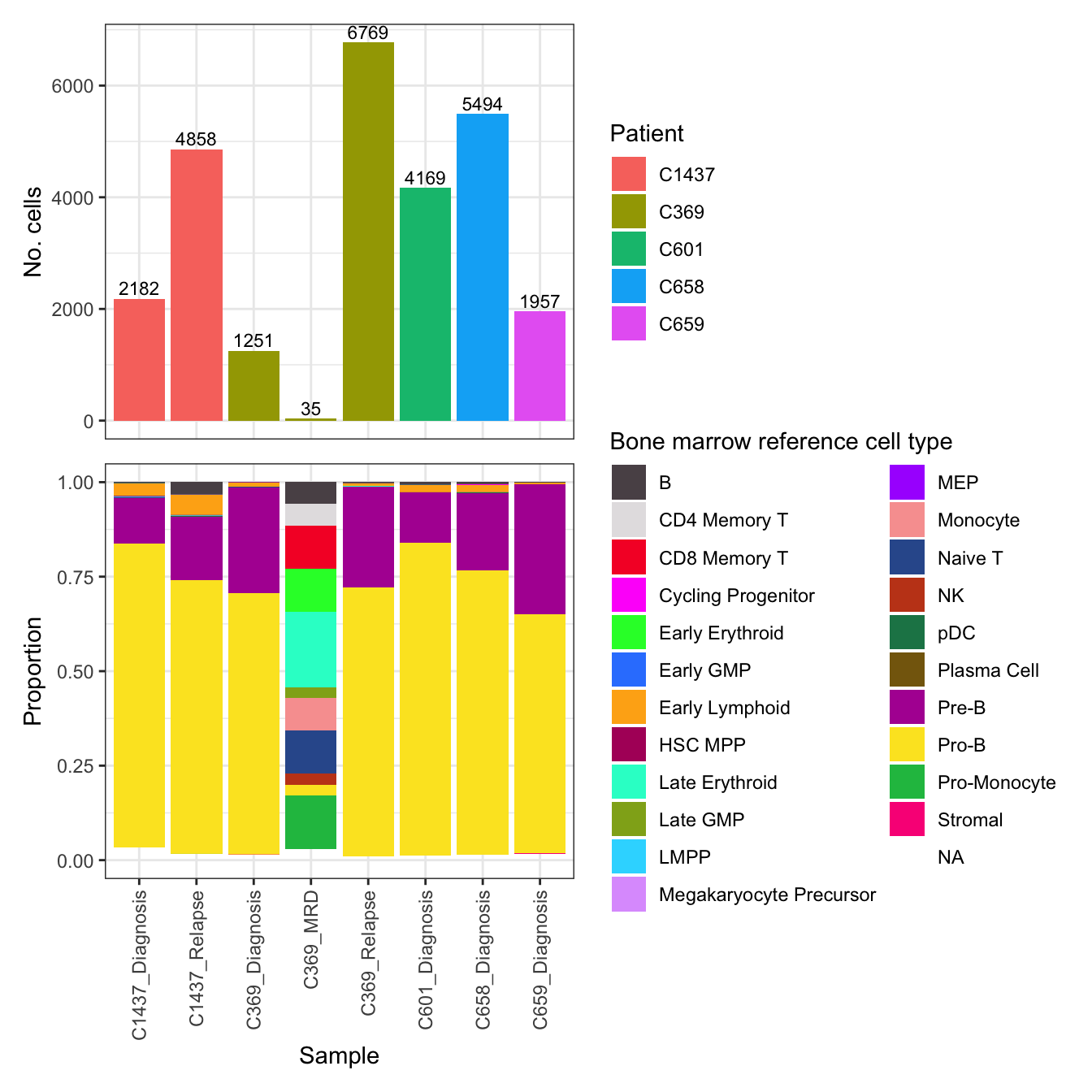

Past versions of plot-fusion-proportion-1.png

Version	Author	Date
1b5bb97	Jovana Maksimovic	2026-05-11

Fusion-positive cells annotated as non-B-precursor cell types are likely ambient contamination. Library size and fusion UMI comparisons help distinguish true blast cells from ambient fusion signal.

seu$suspected_ambient <- seu$patient_fusion != "not-detected" &
  !seu$predicted_CellType_Broad %in% c("Pro-B", "Pre-B", "Early Lymphoid")

VlnPlot(seu, features = "nCount_RNA", 
        group.by = "suspected_ambient",
        pt.size = 0)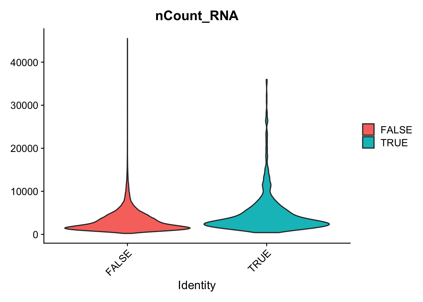

Past versions of identify-blast-cells-1.png

Version	Author	Date
1b5bb97	Jovana Maksimovic	2026-05-11

# Add a flag for suspected ambient fusion-positive cells
b_precursor_types <- c("Pro-B", "Pre-B", "Early Lymphoid")

seu$fusion_classification <- case_when(
  seu$patient_fusion == "not-detected" ~ "not-detected",
  seu$predicted_CellType_Broad %in% b_precursor_types ~ "fusion-positive blast",
  TRUE ~ "fusion-positive non-blast"
)

# UMI comparison
VlnPlot(seu, 
        features = "nCount_RNA",
        group.by = "fusion_classification",
        pt.size = 0.1) +
  scale_y_log10()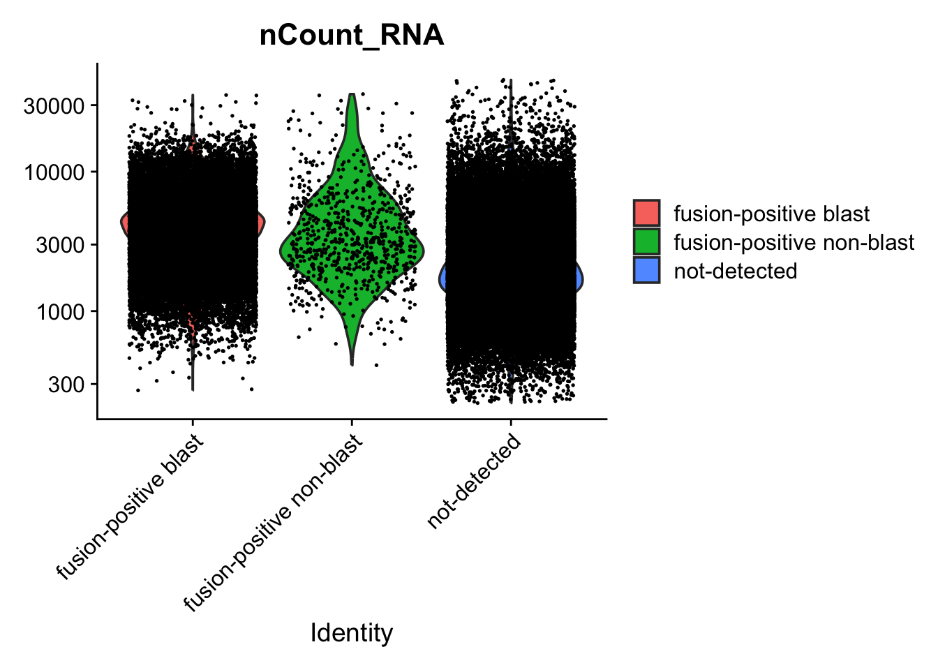

Past versions of flag-ambient-fusion-1.png

Version	Author	Date
1b5bb97	Jovana Maksimovic	2026-05-11

# Extract fusion UMI counts per cell
seu$fusion_v1_UMI <- GetAssayData(seu, layer = "counts")["ETV6-RUNX1-v1-fusion", ]
seu$fusion_v2_UMI <- GetAssayData(seu, layer = "counts")["ETV6-RUNX1-v2-fusion", ]
seu$fusion_total_UMI <- seu$fusion_v1_UMI + seu$fusion_v2_UMI

# Compare fusion UMI counts between blast and non-blast fusion-positive cells
VlnPlot(seu %>% subset(patient_fusion != "not-detected"),
        features = "fusion_total_UMI",
        group.by = "fusion_classification",
        pt.size = 0.5) +
  scale_y_log10()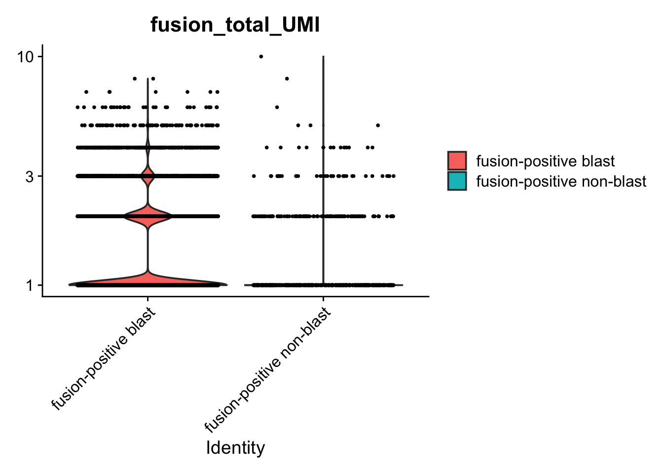

Past versions of compare-fusion-umi-1.png

Version	Author	Date
1b5bb97	Jovana Maksimovic	2026-05-11

seu@meta.data %>%
  filter(patient_fusion != "not-detected") %>%
  group_by(fusion_classification) %>%
  summarise(
    n = n(),
    median_fusion_UMI = median(fusion_total_UMI),
    mean_fusion_UMI = mean(fusion_total_UMI),
    pct_1UMI = mean(fusion_total_UMI == 1) * 100
  )

# A tibble: 2 × 5
  fusion_classification         n median_fusion_UMI mean_fusion_UMI pct_1UMI
  <chr>                     <int>             <dbl>           <dbl>    <dbl>
1 fusion-positive blast     25963                 1            1.40     70.7
2 fusion-positive non-blast   752                 1            1.34     77.8

seu@meta.data %>%
  filter(patient_fusion != "not-detected") %>%
  group_by(predicted_CellType_Broad, fusion_classification) %>%
  summarise(
    n = n(),
    median_fusion_UMI = median(fusion_total_UMI),
    pct_1UMI = mean(fusion_total_UMI == 1) * 100
  ) %>%
  arrange(fusion_classification, desc(n))

# A tibble: 23 × 5
# Groups:   predicted_CellType_Broad [23]
   predicted_CellType_B…¹ fusion_classification     n median_fusion_UMI pct_1UMI
   <chr>                  <chr>                 <int>             <dbl>    <dbl>
 1 Pro-B                  fusion-positive blast 19791                 1     70.9
 2 Pre-B                  fusion-positive blast  5584                 1     70.0
 3 Early Lymphoid         fusion-positive blast   588                 1     71.6
 4 <NA>                   fusion-positive non-…   394                 1     72.1
 5 B                      fusion-positive non-…   244                 1     84.8
 6 Cycling Progenitor     fusion-positive non-…    18                 1     66.7
 7 pDC                    fusion-positive non-…    15                 2     46.7
 8 Late Erythroid         fusion-positive non-…    11                 1     90.9
 9 Naive T                fusion-positive non-…    10                 1    100  
10 Early Erythroid        fusion-positive non-…     9                 1    100  
# ℹ 13 more rows
# ℹ abbreviated name: ¹​predicted_CellType_Broad

CD19 expression

VlnPlot(seu[, seu$fusion_detected], 
        features = "CD19", 
        group.by = "predicted_CellType_Broad", 
        split.by = "patient_timepoint") +
  theme(legend.position = "bottom")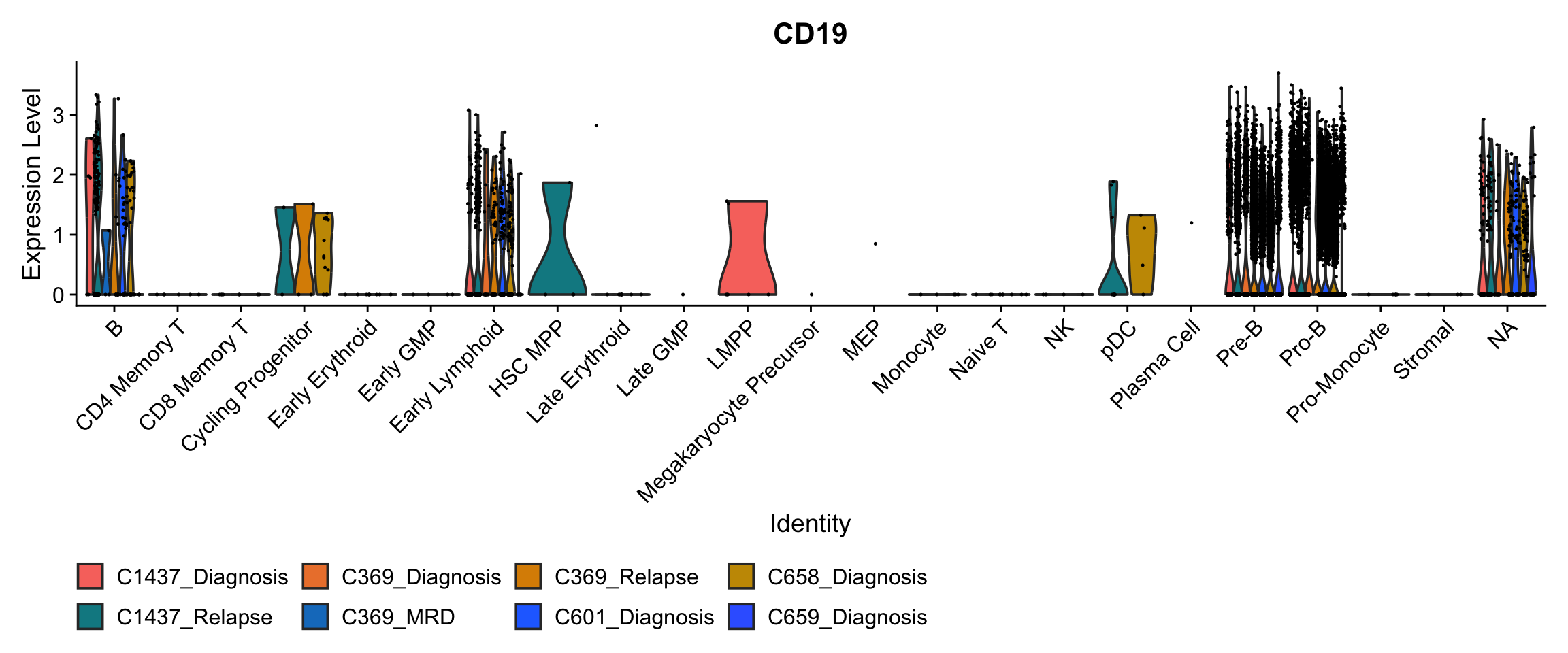

Past versions of plot-cd19-1.png

Version	Author	Date
1b5bb97	Jovana Maksimovic	2026-05-11

Unsupervised clustering

Cell cycle phase is scored before clustering. Each sample is then clustered independently using SCTransform normalisation and Leiden algorithm across a range of resolutions.

s.genes <- cc.genes$s.genes
g2m.genes <- cc.genes$g2m.genes

seu <- CellCycleScoring(seu, 
                        s.features = s.genes, 
                        g2m.features = g2m.genes)

seu@meta.data %>%
    ggplot(aes(x = Phase, 
                           fill = fusion_detected)) +
    geom_bar(position = position_dodge(width = 0.9)) + 
  theme_bw() +
    labs(x = "Sample",
         y = "No. cells",
         fill = "Fusion detected") +
  geom_text(
    stat = "count",
    aes(label = after_stat(count)),
    vjust = -0.5,
    size = 3,
    position = position_dodge(width = 0.9))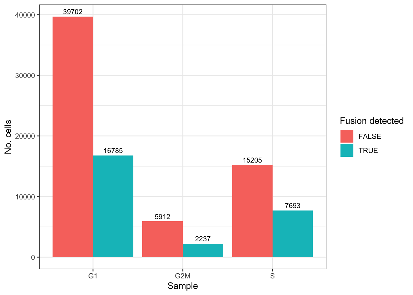

Past versions of normalise-cluster-1.png

Version	Author	Date
1b5bb97	Jovana Maksimovic	2026-05-11

seu@meta.data %>%
  filter(!is.na(Phase)) %>%
  group_by(Phase) %>%
  summarise(
    total = n(),
    fusion_positive = sum(patient_fusion != "not-detected"),
    pct_fusion = round(fusion_positive / total * 100, 1),
    .groups = "drop"
  ) %>%
  mutate(
    label = paste0(pct_fusion, "%"),
    Phase = factor(Phase, levels = c("G1", "S", "G2M"))
  ) %>%
  ggplot(aes(x = Phase, y = pct_fusion, fill = Phase)) +
  geom_col(width = 0.5) +
  geom_text(aes(label = label), vjust = -0.5, size = 3.5) +
  scale_fill_manual(values = c(
    "G1"  = "#E69F00",
    "S"   = "#009E73",
    "G2M" = "#56B4E9"
  )) +
  scale_y_continuous(limits = c(0, 45), expand = c(0, 0)) +
  labs(x = "Cell cycle phase", y = "% fusion-positive cells") +
  theme_classic() +
  theme(legend.position = "none")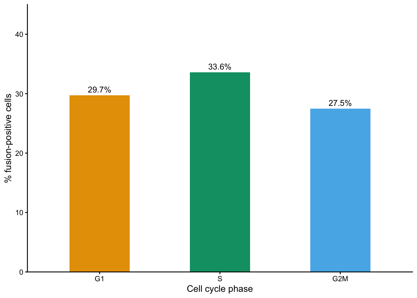

Past versions of find-clusters-1.png

Version	Author	Date
1b5bb97	Jovana Maksimovic	2026-05-11

Cluster each sample individually at multiple resolutions, to identify the leukaemic cell population.

out <- here("data", "RDS", "ball_exp2_clustered.seu.rds")

if(!file.exists(out)) {
  
  seu[["RNA"]] <- split(seu[["RNA"]], f = factor(seu$batch))
  
  seu <- SCTransform(seu, verbose = FALSE,
                       return.only.var.genes = TRUE)#,
                       #vars.to.regress = c("S.Score", "G2M.Score", "nCount_RNA"))
  
  seu_lst <- SplitObject(seu, split.by = "patient_timepoint")
  
  lapply(seu_lst, function(seu){
    # seu <- SCTransform(seu, verbose = FALSE,
    #                    return.only.var.genes = FALSE,
    #                    vars.to.regress = c("S.Score", "G2M.Score", "nCount_RNA"))
    
    DefaultAssay(seu) <- "SCT"
    seu <- FindVariableFeatures(seu)
    #VariableFeatures(seu) <- setdiff(VariableFeatures(seu), c(s.genes, g2m.genes))
    seu <- RunPCA(seu, verbose = FALSE, npcs = 30, assay = "SCT")
    seu <- RunUMAP(seu, dims = 1:30, reduction = "pca")
    
    seu <- FindNeighbors(seu, reduction = "pca", dims = 1:30)
    seu <- FindClusters(seu, resolution = seq(0.1, 1, by = 0.1),
                        algorithm = "Leiden")
    seu
    
  }) -> seu_lst
  
  saveRDS(seu_lst, file = out)
  fs::file_chmod(out, "664")
  try(fs::file_chown(out, group_id = "oshlack_lab"),
      silent = TRUE)

} else {
  seu_lst <- readRDS(out)

}

Select resolution

The lowest resolution (0.3) is probably sufficient for separating likely leukaemic clusters from clusters of other cells.

lapply(seu_lst, function(seu){
  clustree(seu, prefix = "SCT_snn_res.")
})

$C659_Diagnosis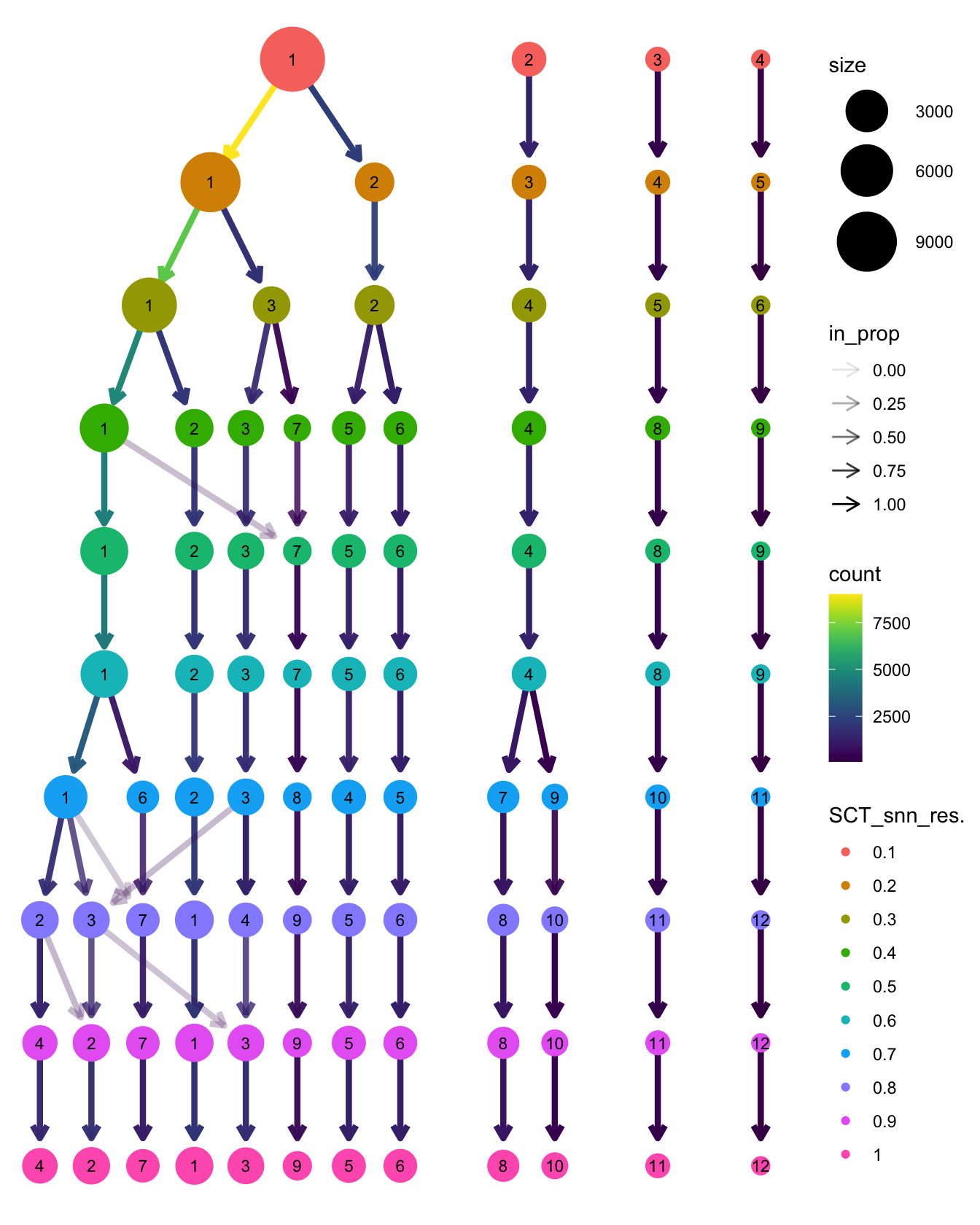

Past versions of plot-clustree-1.png

Version	Author	Date
1b5bb97	Jovana Maksimovic	2026-05-11

$C1437_Relapse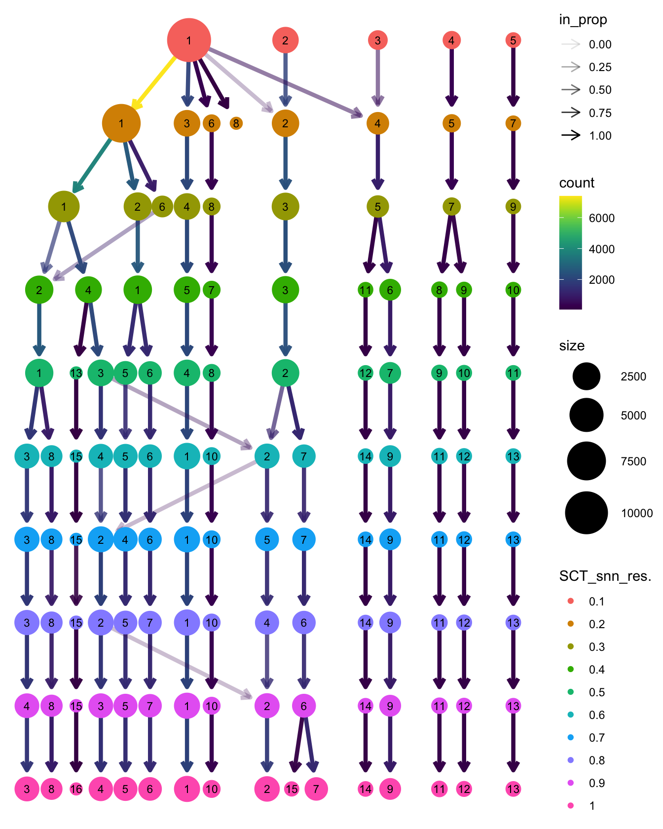

Past versions of plot-clustree-2.png

Version	Author	Date
1b5bb97	Jovana Maksimovic	2026-05-11

$C369_Diagnosis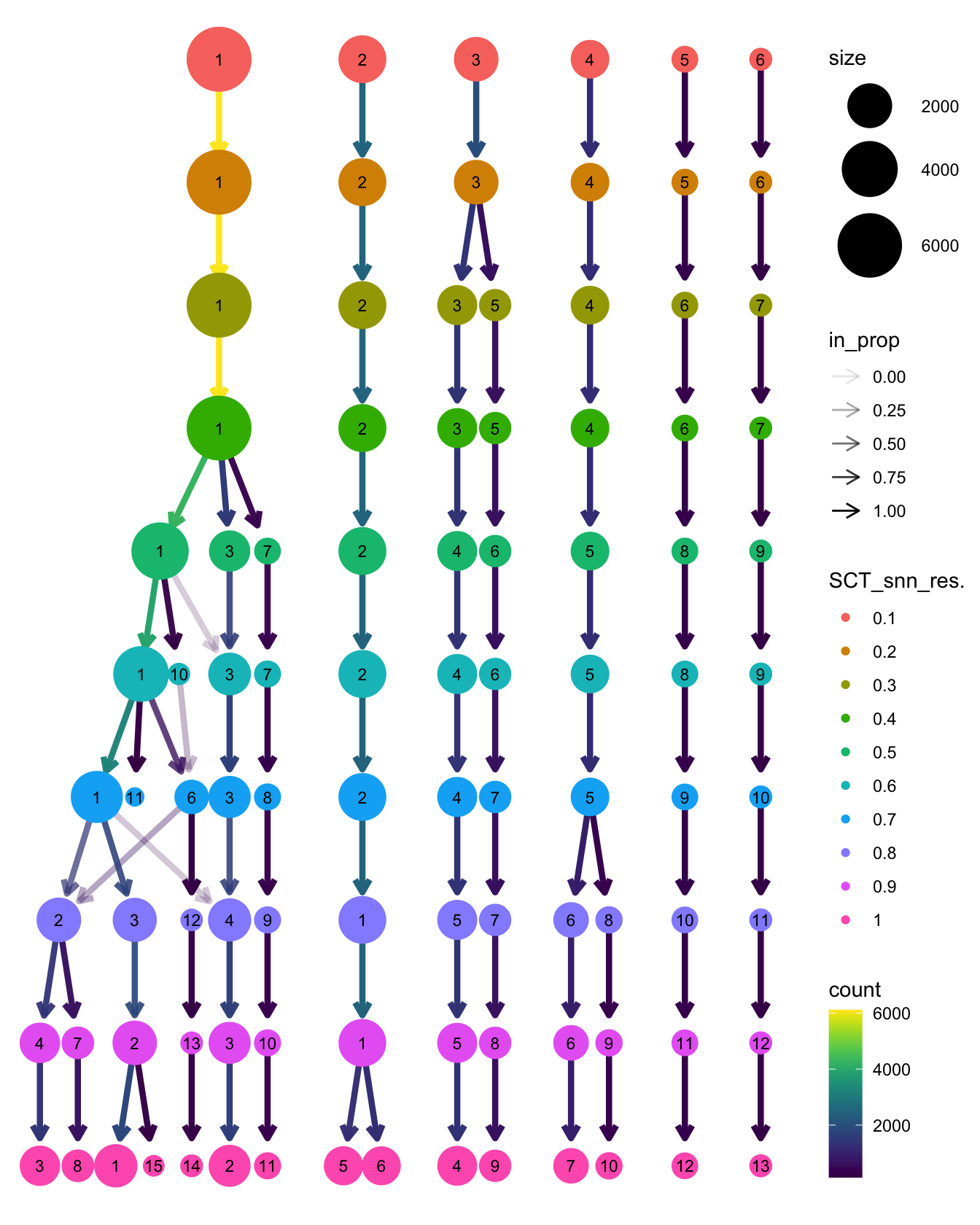

Past versions of plot-clustree-3.png

Version	Author	Date
1b5bb97	Jovana Maksimovic	2026-05-11

$C1437_Diagnosis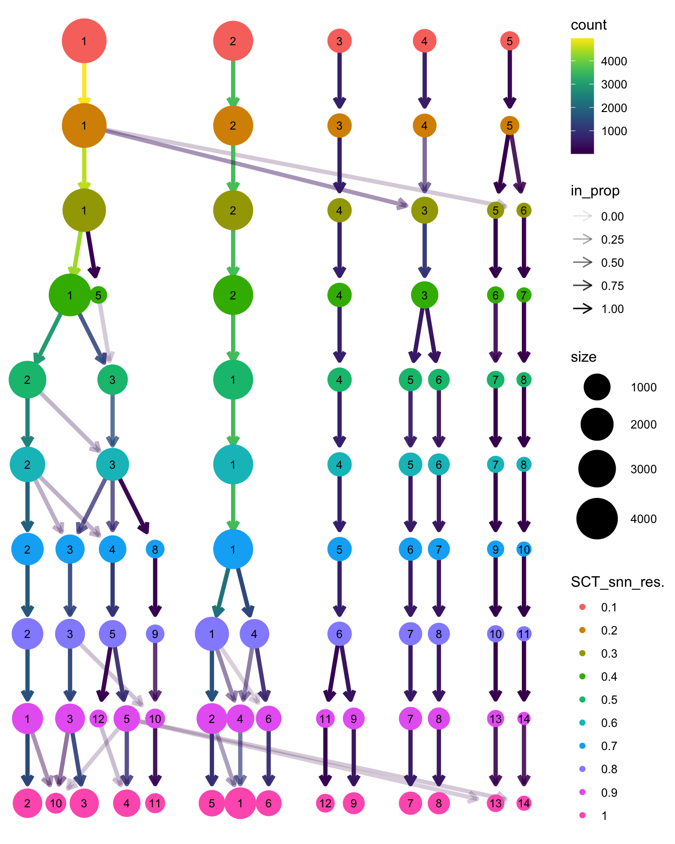

Past versions of plot-clustree-4.png

Version	Author	Date
1b5bb97	Jovana Maksimovic	2026-05-11

$C369_Relapse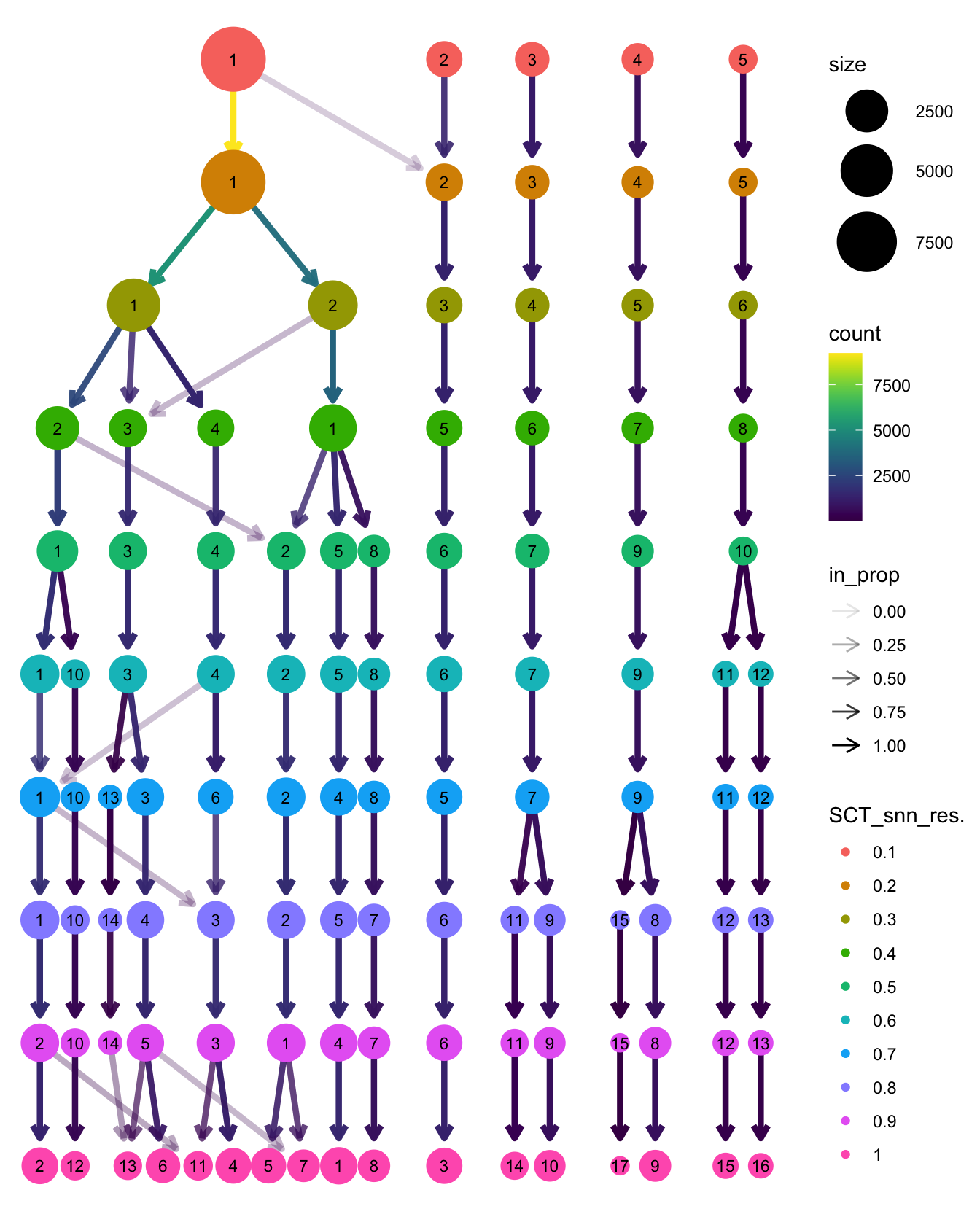

Past versions of plot-clustree-5.png

Version	Author	Date
1b5bb97	Jovana Maksimovic	2026-05-11

$C658_Diagnosis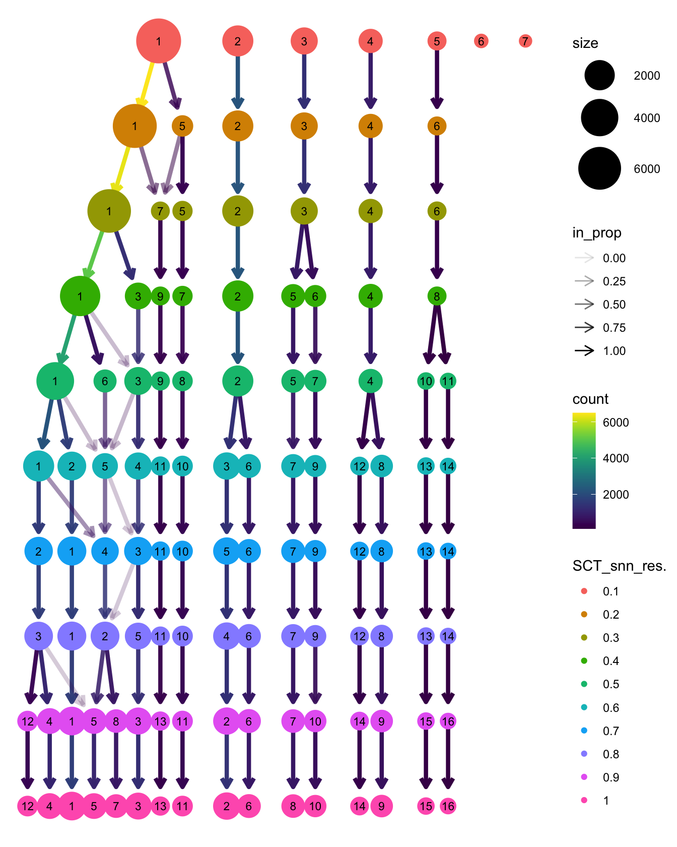

Past versions of plot-clustree-6.png

Version	Author	Date
1b5bb97	Jovana Maksimovic	2026-05-11

$C601_Diagnosis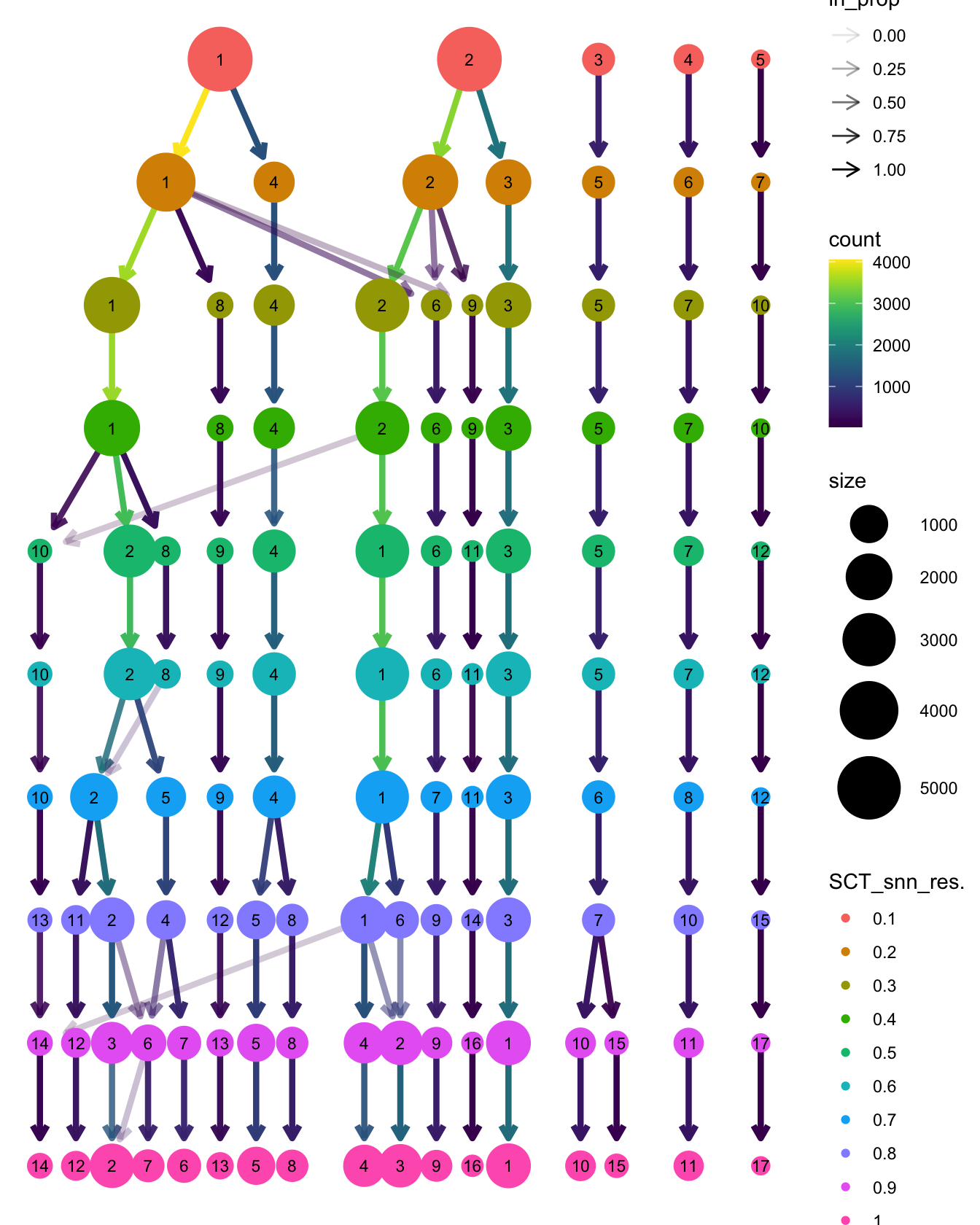

Past versions of plot-clustree-7.png

Version	Author	Date
1b5bb97	Jovana Maksimovic	2026-05-11

$C369_MRD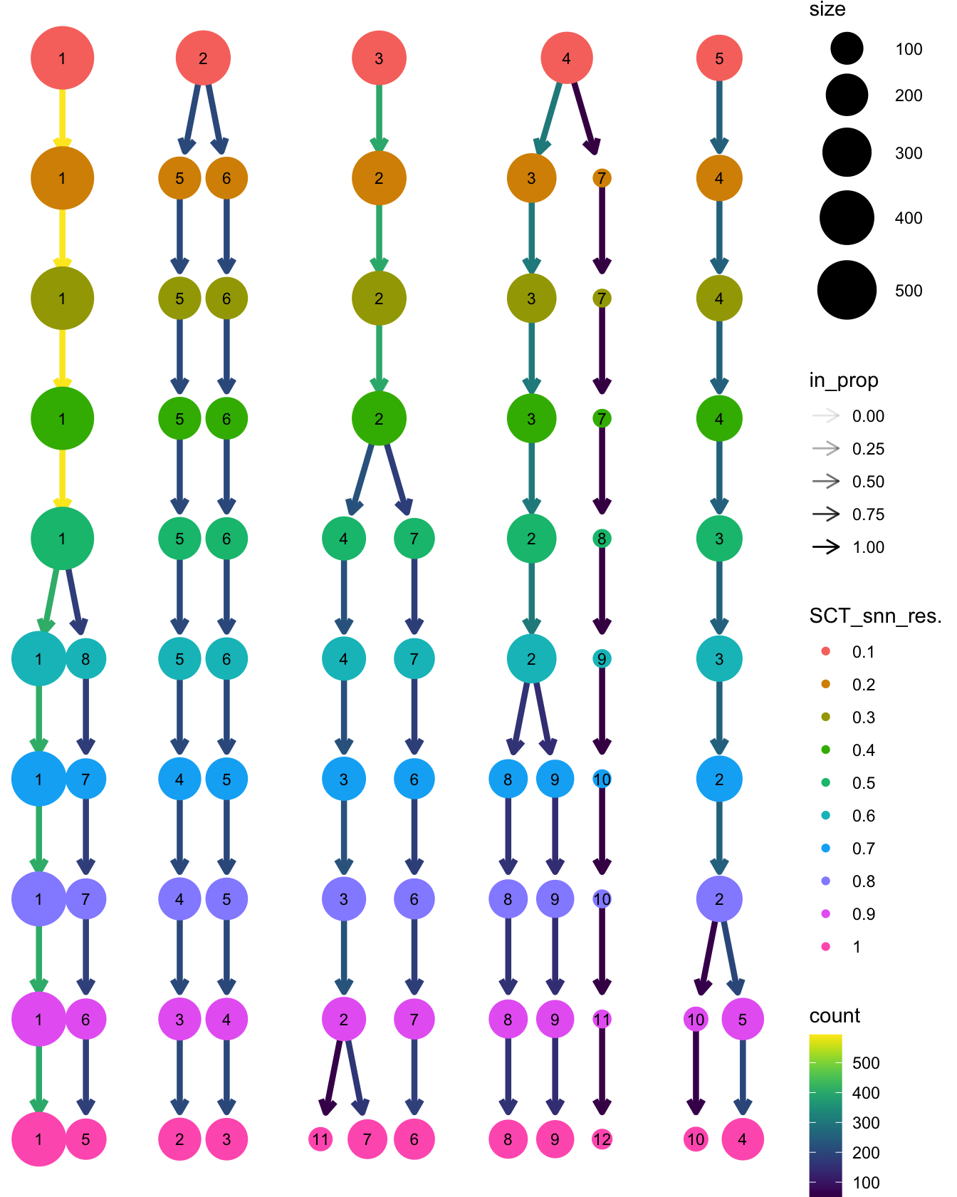

Past versions of plot-clustree-8.png

Version	Author	Date
1b5bb97	Jovana Maksimovic	2026-05-11

Examine UMAPs

Visualise the clusters for each sample, along with cell cycle, labelled fusions and broad reference annotations.

grp <- "SCT_snn_res.0.3"

lapply(seq_along(seu_lst), function(i){
  DimPlot(seu_lst[[i]], reduction = "umap", label = TRUE, repel = TRUE,
          label.size = 2.5, group.by = grp) +
    theme(legend.text = element_text(size = 8),
          legend.position = "bottom") -> p1
  
    DimPlot(seu_lst[[i]], reduction = "umap", label = TRUE, repel = TRUE,
          label.size = 2.5, group.by = grp, 
          cells.highlight = which(seu_lst[[i]]$patient_fusion != "not-detected"),
          sizes.highlight = 0.1) +
    NoLegend() -> p2
    
    DimPlot(seu_lst[[i]], reduction = "umap", label = TRUE, repel = TRUE,
          label.size = 2.5, group.by = "predicted_CellType_Broad") +
    NoLegend() -> p3
  
    DimPlot(seu_lst[[i]], reduction = "umap", label = TRUE, repel = TRUE,
          label.size = 2.5, group.by = "Phase") +
    theme(legend.text = element_text(size = 8),
          legend.position = "bottom") -> p4
    
  ((p1 | p4) / (p2 | p3)) + 
      plot_annotation(title = names(seu_lst)[i]) +
      theme(title = element_text(size = 10))
}) -> p

p

[[1]]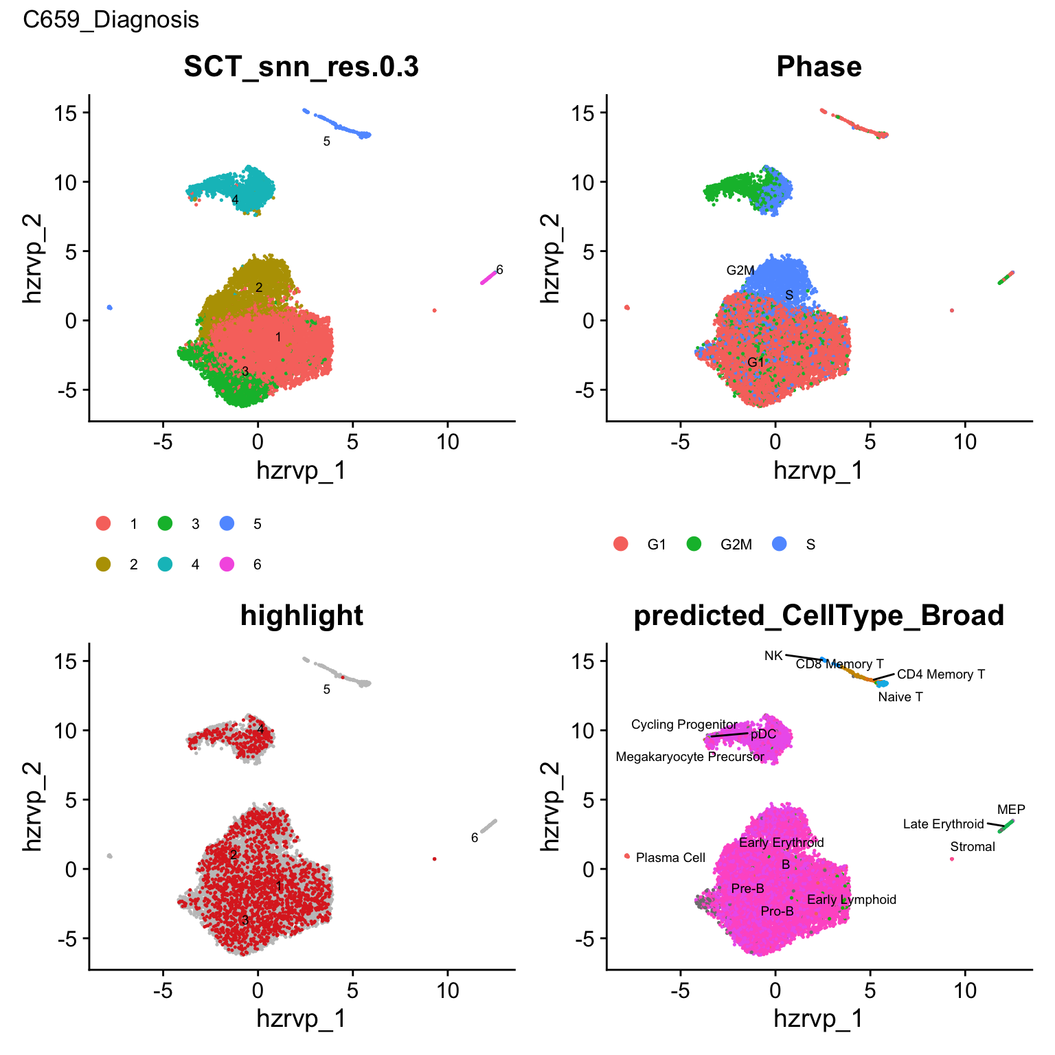

Past versions of plot-cluster-umap-1.png

Version	Author	Date
1b5bb97	Jovana Maksimovic	2026-05-11

[[2]]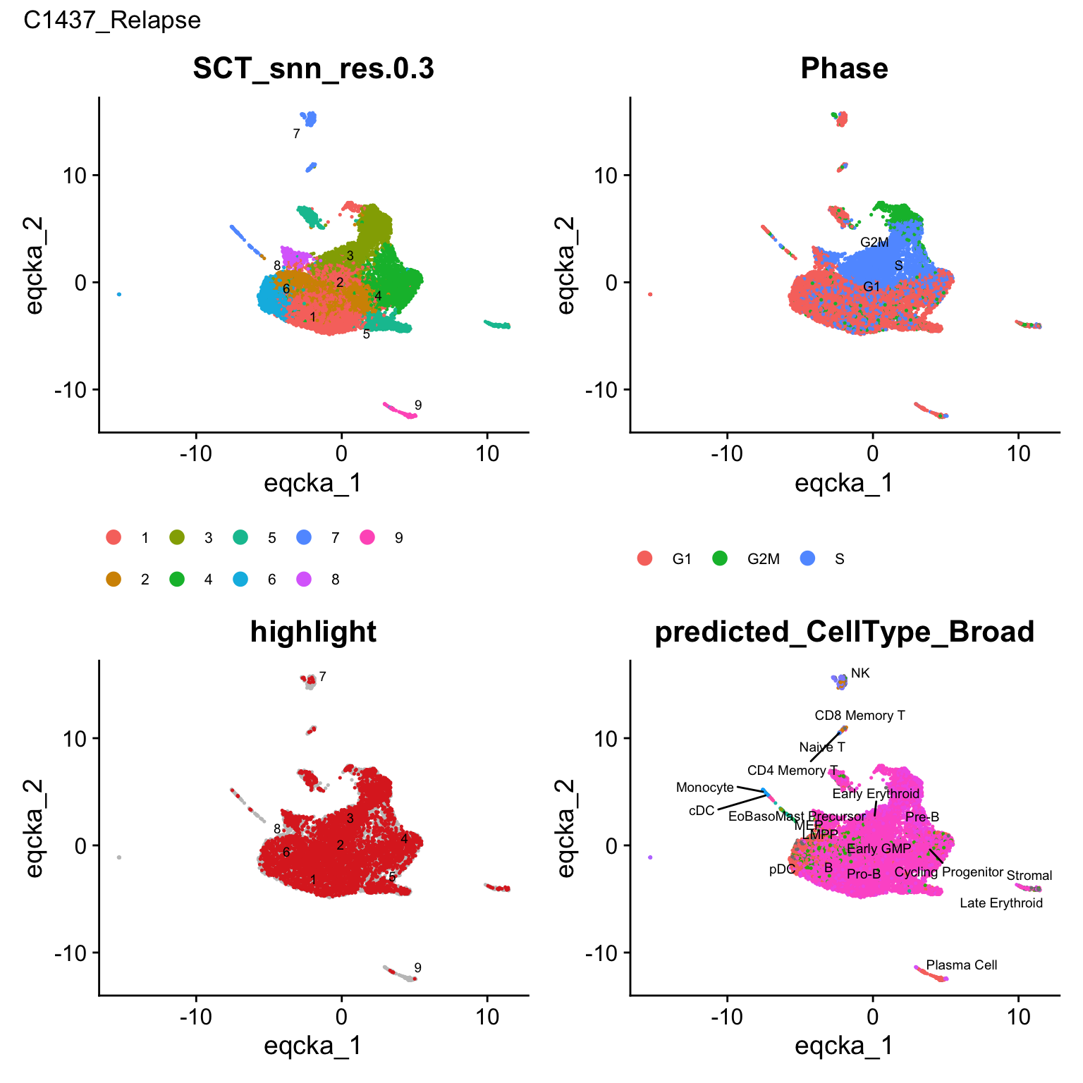

Past versions of plot-cluster-umap-2.png

Version	Author	Date
1b5bb97	Jovana Maksimovic	2026-05-11

[[3]]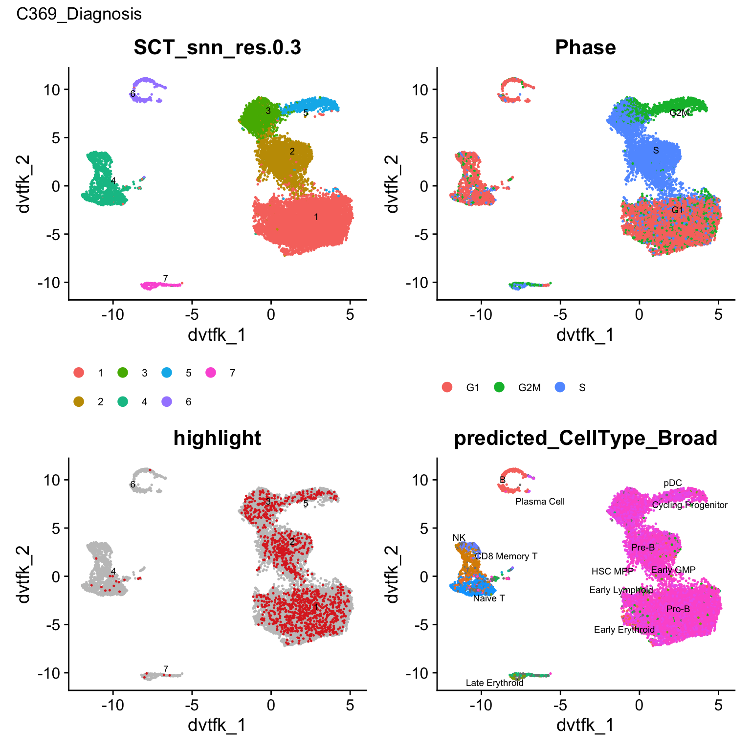

Past versions of plot-cluster-umap-3.png

Version	Author	Date
1b5bb97	Jovana Maksimovic	2026-05-11

[[4]]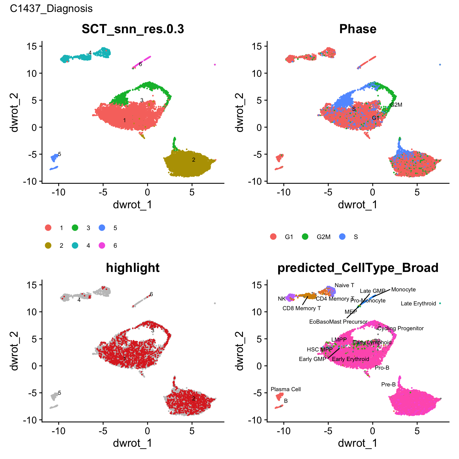

Past versions of plot-cluster-umap-4.png

Version	Author	Date
1b5bb97	Jovana Maksimovic	2026-05-11

[[5]]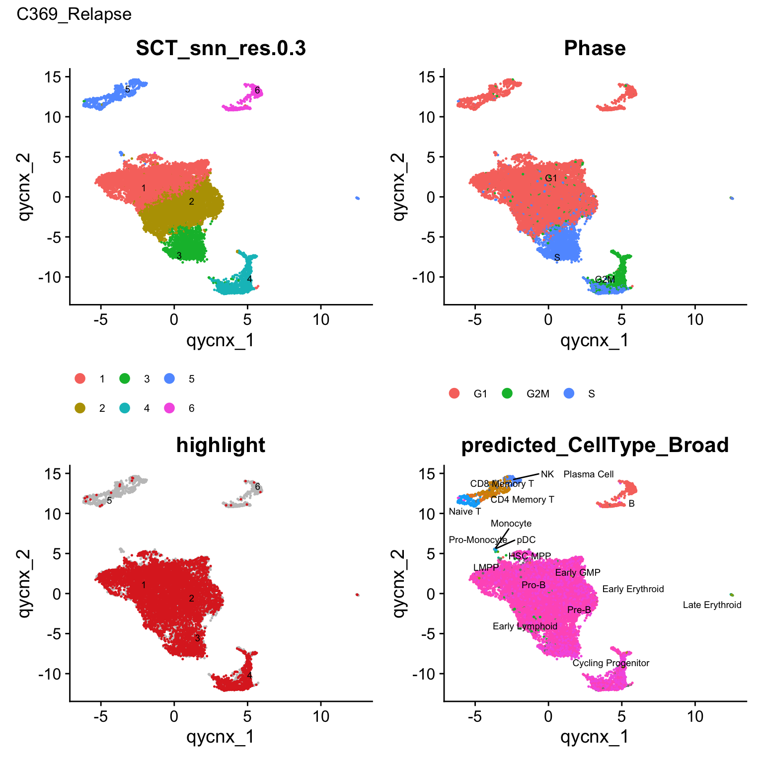

Past versions of plot-cluster-umap-5.png

Version	Author	Date
1b5bb97	Jovana Maksimovic	2026-05-11

[[6]]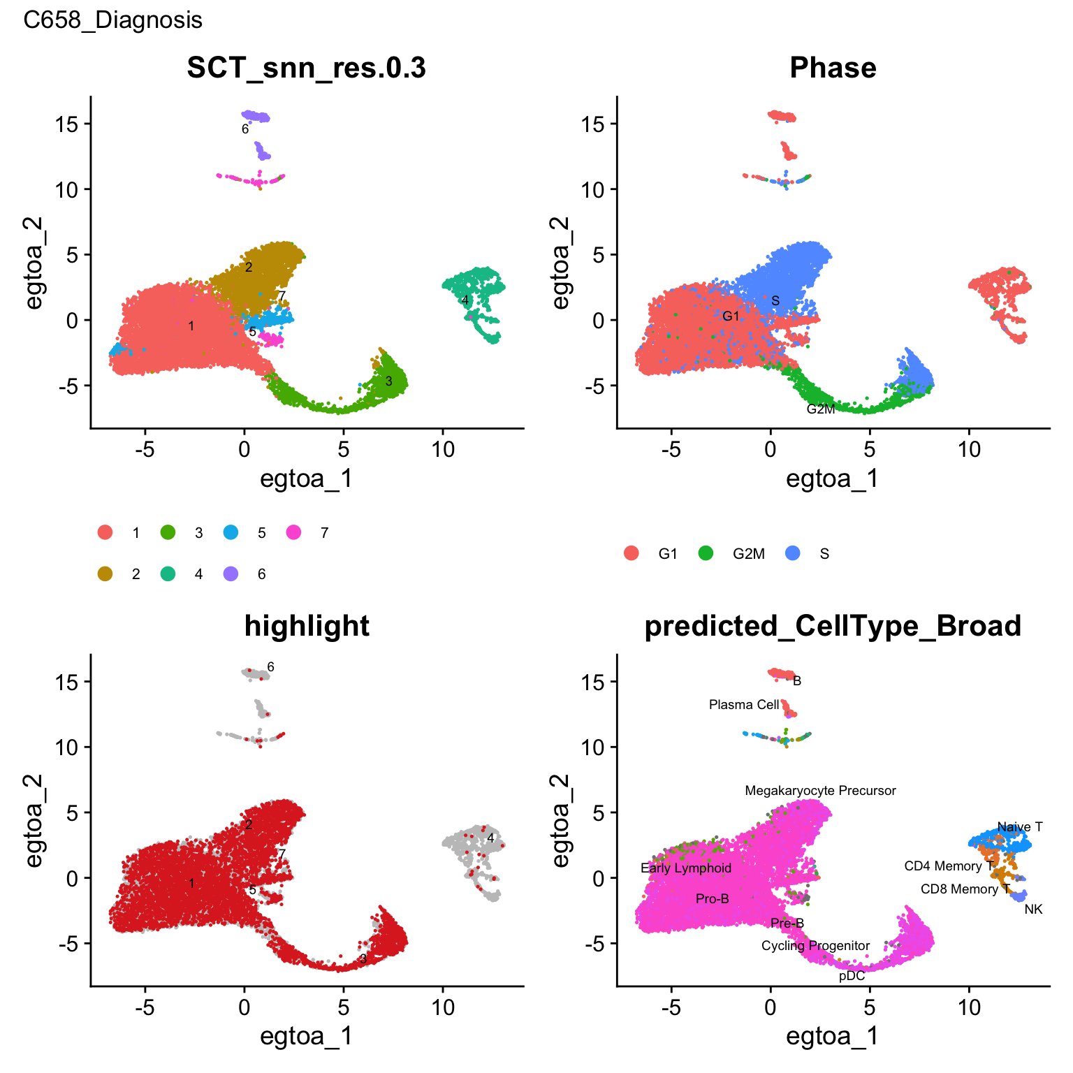

Past versions of plot-cluster-umap-6.png

Version	Author	Date
1b5bb97	Jovana Maksimovic	2026-05-11

[[7]]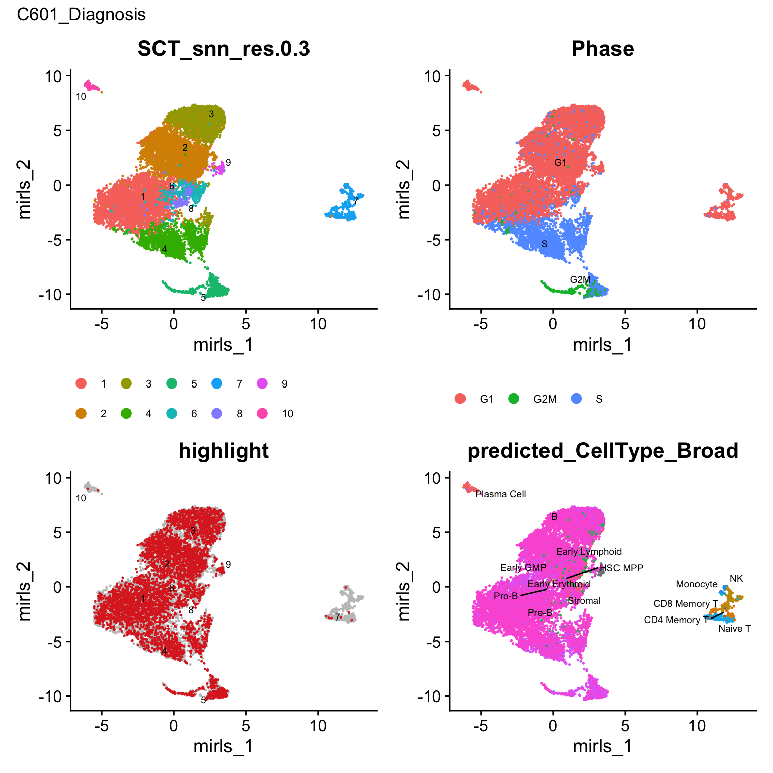

Past versions of plot-cluster-umap-7.png

Version	Author	Date
1b5bb97	Jovana Maksimovic	2026-05-11

[[8]]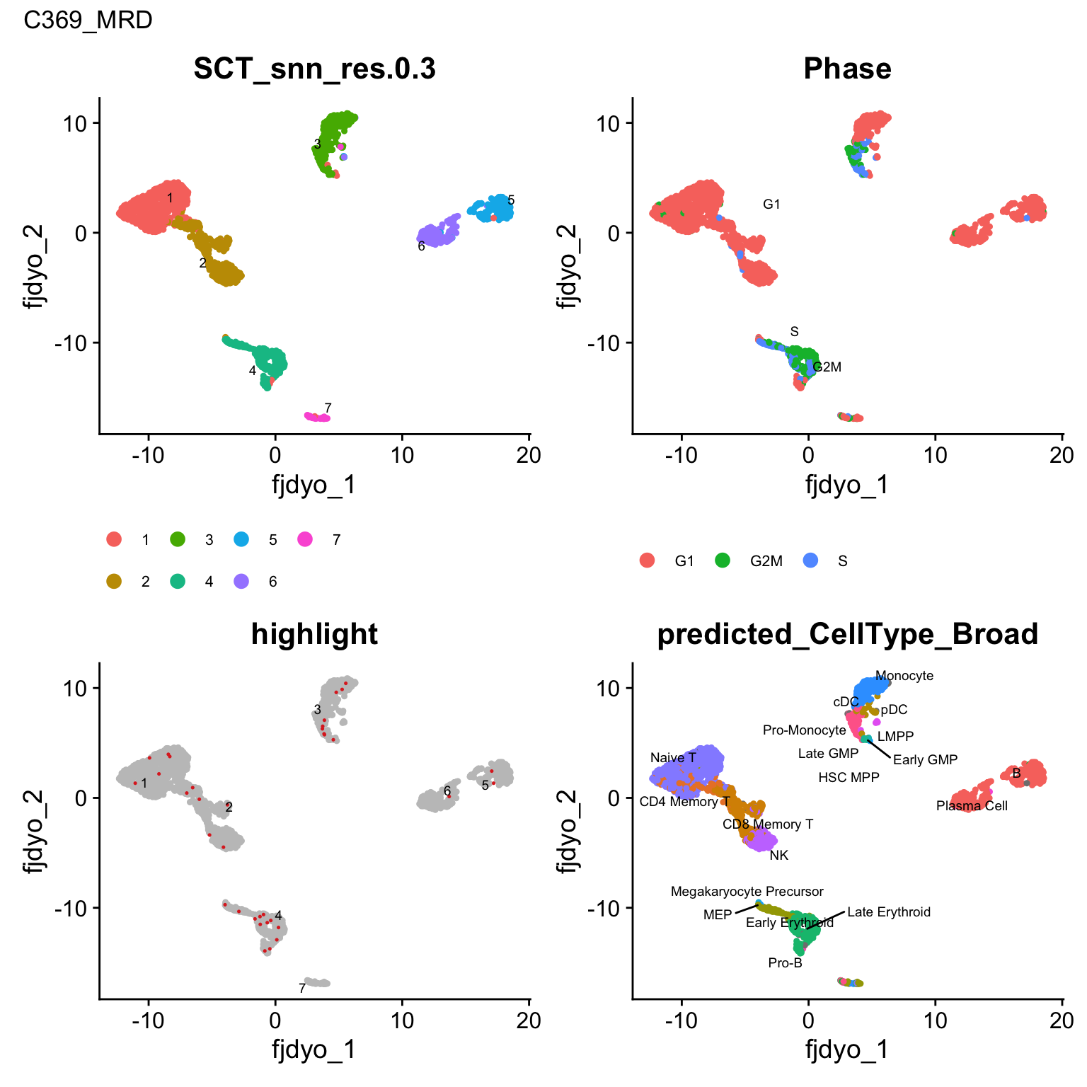

Past versions of plot-cluster-umap-8.png

Version	Author	Date
1b5bb97	Jovana Maksimovic	2026-05-11

Per-sample four-panel UMAPs (clusters, cell cycle, fusion highlight, BoneMarrowMap annotation) for all eight samples. This figure was previously Supplementary Figure 6 but has been retired from the active figure set; it is retained here as a diagnostic overview.

# Exploratory per-sample clustering: clusters, cell cycle, fusion, and BoneMarrowMap annotation for all eight Exp2 samples
grp <- "SCT_snn_res.0.3"

lapply(seq_along(seu_lst), function(i) {
  
  # Cluster UMAP
  DimPlot(seu_lst[[i]], reduction = "umap", label = TRUE, repel = TRUE,
          label.size = 2.5, group.by = grp) +
    theme(legend.text = element_text(size = 8),
          legend.position = "bottom") +
    NoAxes() -> p1
  
  # Cell cycle phase
  DimPlot(seu_lst[[i]], reduction = "umap", label = TRUE, repel = TRUE,
          label.size = 2.5, group.by = "Phase") +
    scale_color_manual(values = c("G1" = "#E69F00", 
                                  "G2M" = "#56B4E9", 
                                  "S" = "#009E73")) +
    theme(legend.text = element_text(size = 8),
          legend.position = "bottom") +
    NoAxes() -> p2
  
  # Fusion highlight
  DimPlot(seu_lst[[i]], reduction = "umap", label = TRUE, repel = TRUE,
          label.size = 2.5, group.by = grp,
          cells.highlight = which(seu_lst[[i]]$patient_fusion != "not-detected"),
          sizes.highlight = 0.1) +
    NoLegend() +
    NoAxes() +
    ggtitle("Fusion highlight") -> p3
  
  # BoneMarrowMap annotation
  DimPlot(seu_lst[[i]], reduction = "umap", label = TRUE, repel = TRUE,
          label.size = 2.5, group.by = "predicted_CellType_Broad") +
    NoLegend() +
    NoAxes() +
    ggtitle("BoneMarrowMap annotation") -> p4
  
  ((p1 | p2) / (p3 | p4)) +
    plot_annotation(title = names(seu_lst)[i],
                    theme = theme(plot.title = element_text(size = 10, 
                                                            face = "bold")))
  
}) -> supp_plots

# Print all panels
supp_plots

[[1]]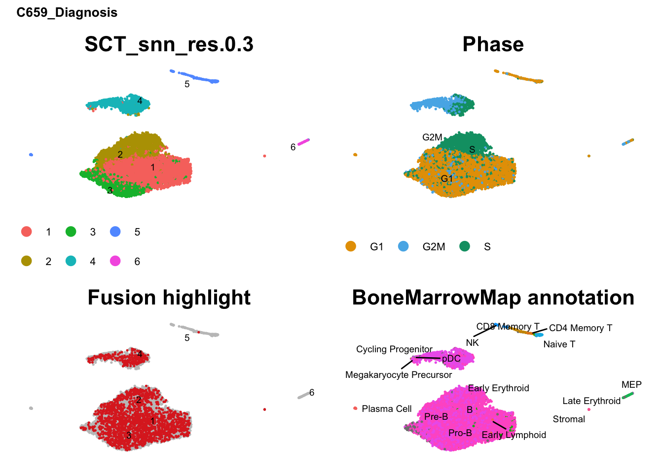

Past versions of fig-supp-per-sample-clustering-1.png

Version	Author	Date
1b5bb97	Jovana Maksimovic	2026-05-11

[[2]]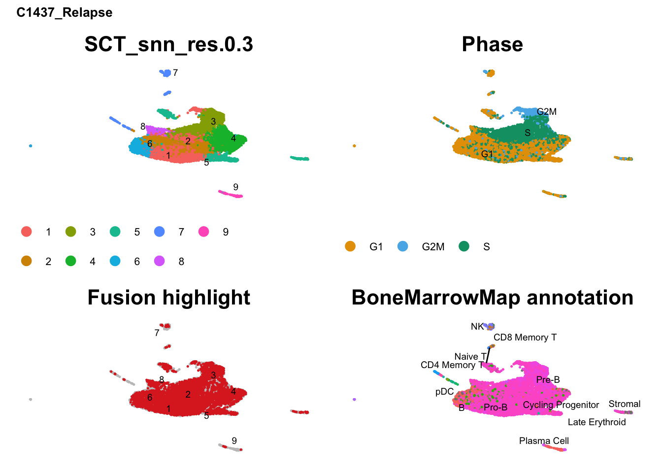

Past versions of fig-supp-per-sample-clustering-2.png

Version	Author	Date
1b5bb97	Jovana Maksimovic	2026-05-11

[[3]]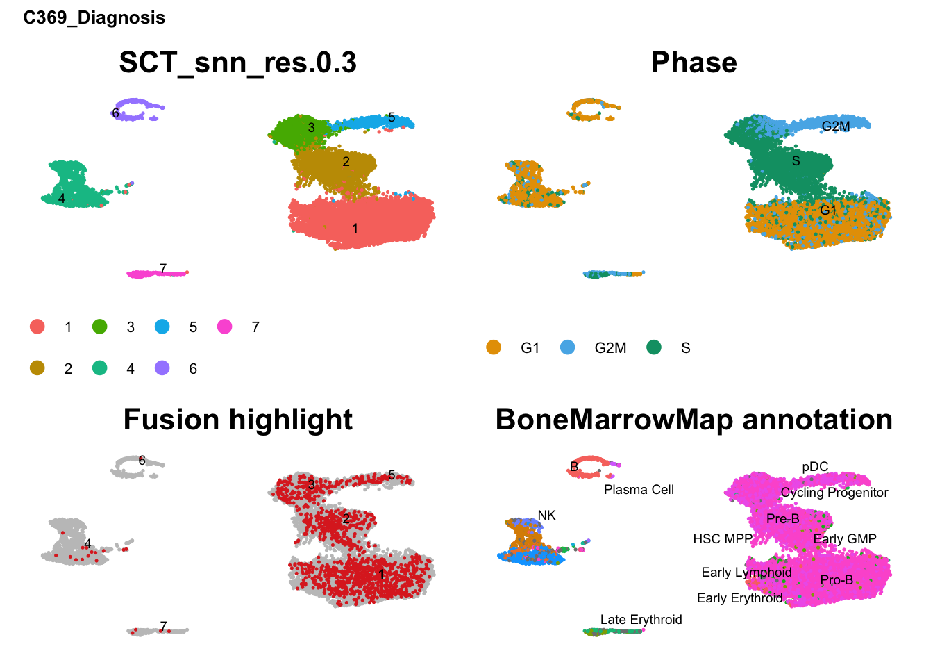

Past versions of fig-supp-per-sample-clustering-3.png

Version	Author	Date
1b5bb97	Jovana Maksimovic	2026-05-11

[[4]]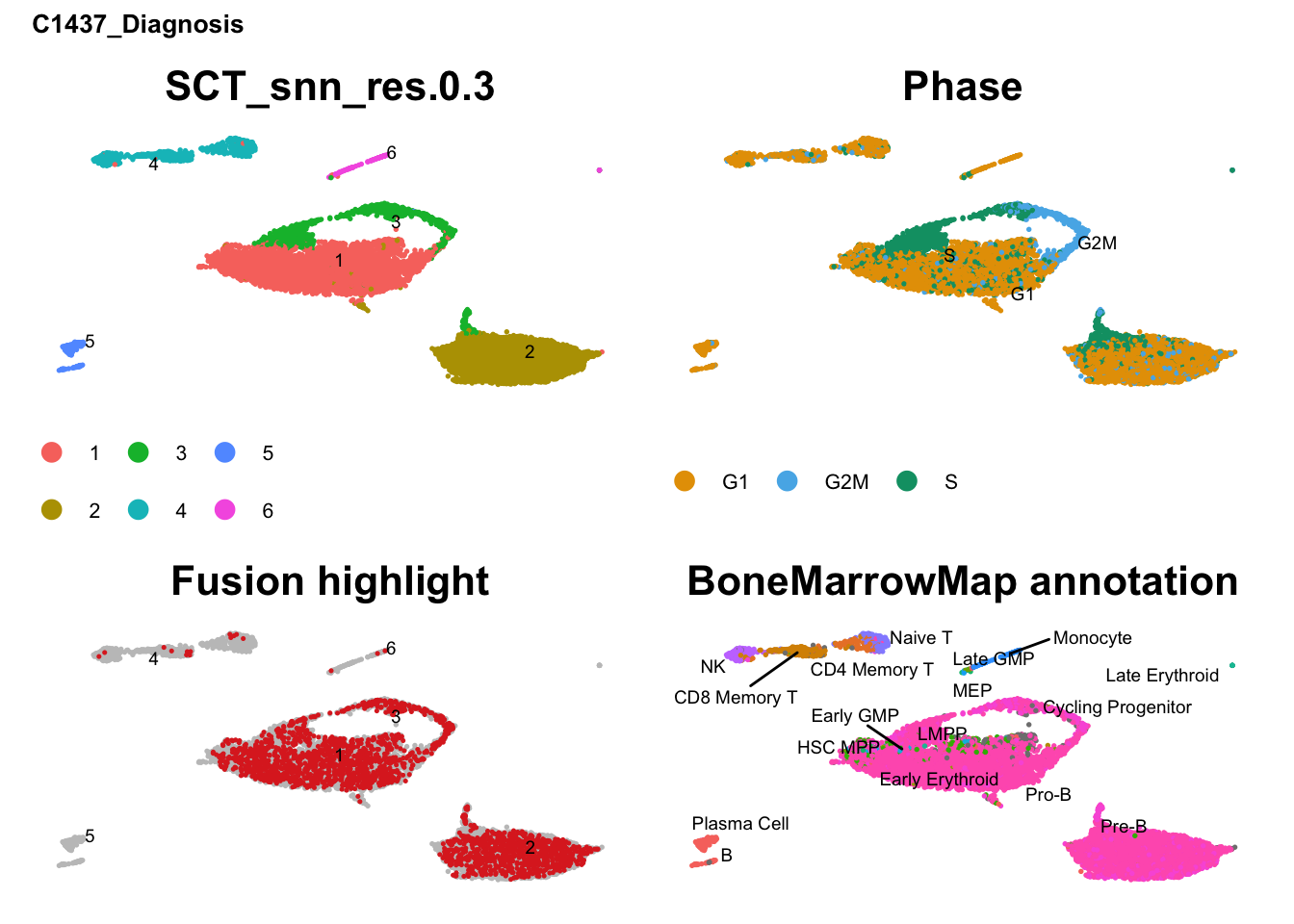

Past versions of fig-supp-per-sample-clustering-4.png

Version	Author	Date
1b5bb97	Jovana Maksimovic	2026-05-11

[[5]]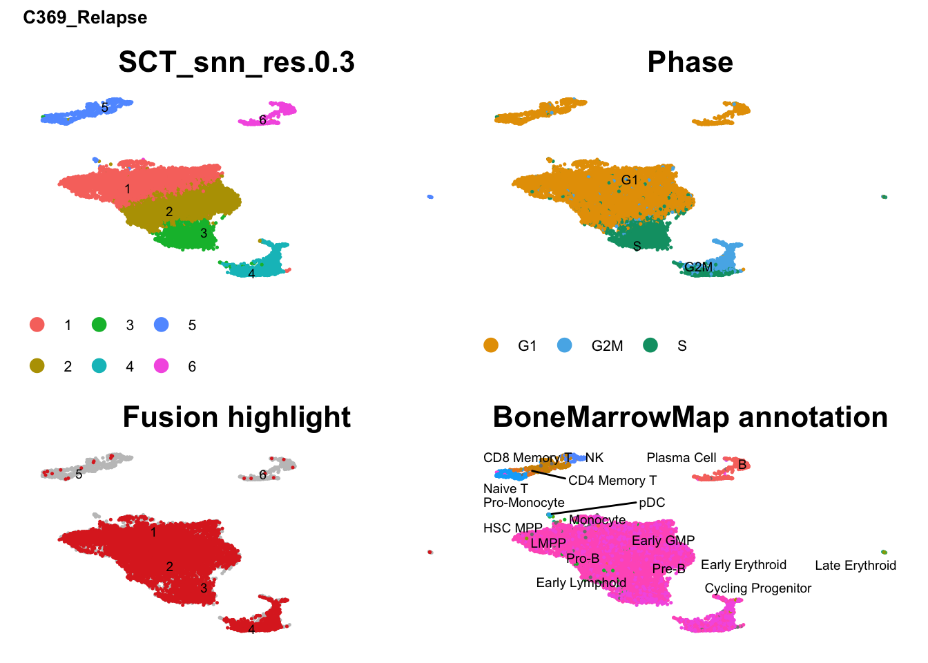

Past versions of fig-supp-per-sample-clustering-5.png

Version	Author	Date
1b5bb97	Jovana Maksimovic	2026-05-11

[[6]]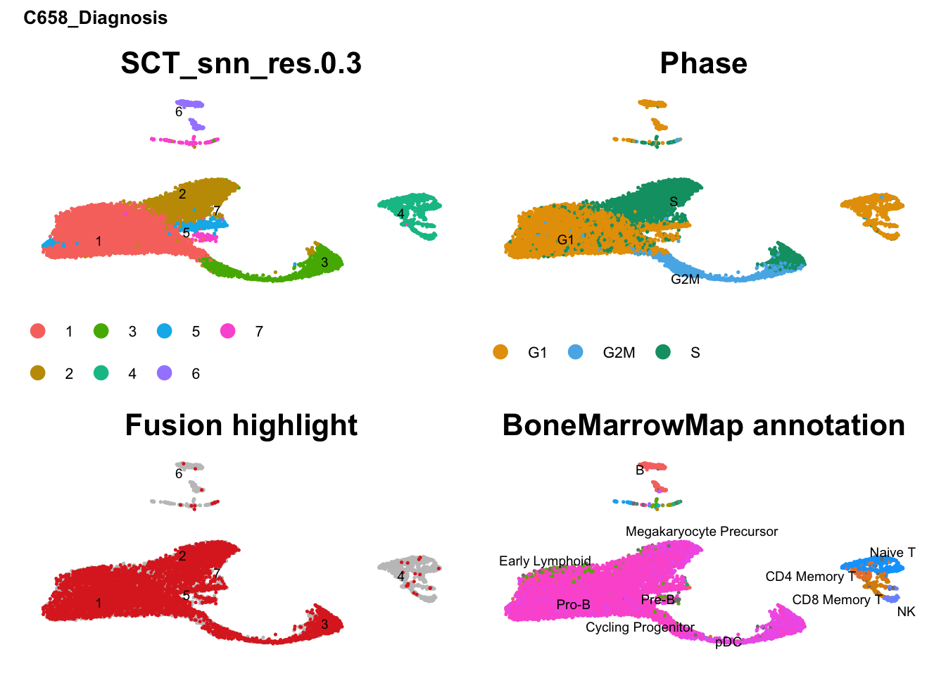

Past versions of fig-supp-per-sample-clustering-6.png

Version	Author	Date
1b5bb97	Jovana Maksimovic	2026-05-11

[[7]]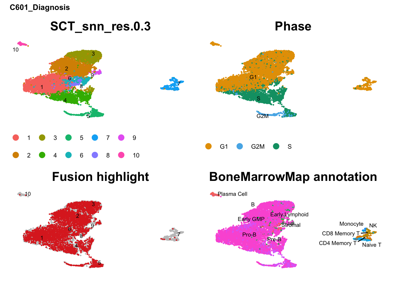

Past versions of fig-supp-per-sample-clustering-7.png

Version	Author	Date
1b5bb97	Jovana Maksimovic	2026-05-11

[[8]]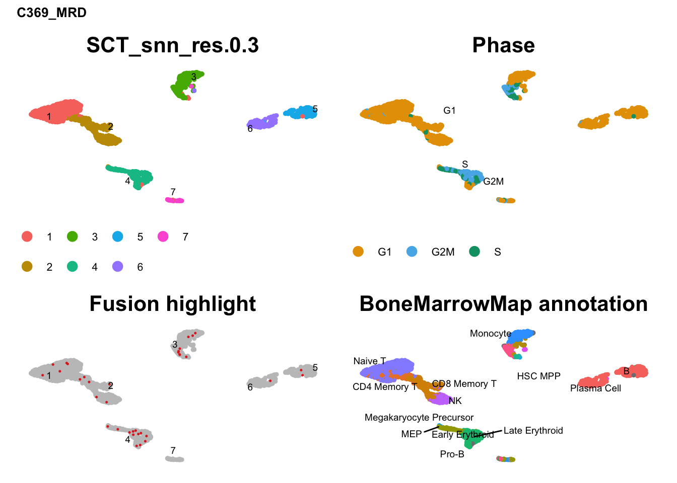

Past versions of fig-supp-per-sample-clustering-8.png

Version	Author	Date
1b5bb97	Jovana Maksimovic	2026-05-11

Publication-quality per-sample figure. For each sample (rows): unsupervised cluster labels, majority-vote cell type annotation, ETV6::RUNX1 fusion isoform highlight, and canonical lineage marker dot plot. Generated separately for Capture 1 (C1437_Dx, C1437_Rel, C369_Dx, C659_Dx) and Capture 2 (C369_Rel, C369_MRD, C601_Dx, C658_Dx) to account for the difference in sequencing depth. This corresponds to Figure 4A.

# Figure 4A: Per-sample four-panel figure (Capture 1 and Capture 2 separately)
# ── Shared themes ─────────────────────────────────────────────────────────────
umap_theme_supp <- function() {
  theme_classic(base_size = 11) +
    theme(
      plot.title       = element_text(size = 11, face = "bold", color = "grey15",
                                      hjust = 0.5, margin = margin(b = 4)),
      axis.title       = element_blank(),
      axis.text        = element_blank(),
      axis.ticks       = element_blank(),
      axis.line        = element_blank(),
      panel.grid       = element_blank(),
      panel.border     = element_blank(),
      legend.text      = element_text(size = 9, color = "grey20"),
      legend.key.size  = unit(0.5, "lines"),
      legend.title     = element_blank(),
      plot.margin      = margin(8, 2, 8, 2)
    )
}

dot_theme_supp <- function() {
  theme_classic(base_size = 9) +
    theme(
      plot.title       = element_text(size = 11, face = "bold", color = "grey15",
                                      hjust = 0.5, margin = margin(b = 4)),
      axis.text.x      = element_text(size = 6, color = "grey20",
                                      angle = 90, hjust = 1, vjust = 0.5),
      axis.text.y      = element_text(size = 7, color = "grey15"),
      axis.title       = element_blank(),
      panel.grid.major = element_line(color = "grey92", linewidth = 0.3),
      legend.text      = element_text(size = 7, color = "grey20"),
      legend.key.size  = unit(0.4, "lines"),
      legend.title     = element_text(size = 7, color = "grey20"),
      plot.margin      = margin(8, 2, 8, 2)
    )
}

col_title_theme <- theme(
  plot.title = element_text(size = 11, face = "bold", color = "grey15",
                            hjust = 0.5, margin = margin(b = 20))
)

# ── Fusion colours ────────────────────────────────────────────────────────────
fusion_colours <- c(
  "ETV6::RUNX1-v1" = "#E69F00",
  "ETV6::RUNX1-v2" = "#0072B2"
)

# ── Canonical markers ─────────────────────────────────────────────────────────
canonical_markers <- c("CD19", "CD3E", "CD14", "HBB", "CD34", "CXCL12")

# ── Sample orders per capture ─────────────────────────────────────────────────
capture1_samples <- c("C1437_Diagnosis", "C1437_Relapse", "C369_Diagnosis", "C659_Diagnosis")
capture2_samples <- c("C369_Relapse", "C369_MRD", "C601_Diagnosis", "C658_Diagnosis")

# ── Core function to build figure for one capture ─────────────────────────────
make_supp_figure <- function(seu_lst_subset) {
  
  # Global max expression for consistent dot plot scale across capture
  global_max_expr <- max(sapply(seu_lst_subset, function(s) {
    avail <- canonical_markers[canonical_markers %in% rownames(s)]
    norm  <- GetAssayData(s, layer = "data")[avail, ]
    max(as.matrix(norm), na.rm = TRUE)
  }))
  
  all_rows <- lapply(seq_along(seu_lst_subset), function(i) {
    
    s       <- seu_lst_subset[[i]]
    s_name  <- names(seu_lst_subset)[i]
    is_last <- i == length(seu_lst_subset)
    
    # ── Majority vote annotation ──────────────────────────────────────────────
    cluster_annotation <- s@meta.data %>%
      tibble::rownames_to_column("cell") %>%
      mutate(
        cluster   = as.character(.data[["SCT_snn_res.0.3"]]),
        cell_type = as.character(predicted_CellType_Broad)
      ) %>%
      group_by(cluster, cell_type) %>%
      summarise(n = n(), .groups = "drop") %>%
      group_by(cluster) %>%
      slice_max(n, n = 1, with_ties = FALSE) %>%
      ungroup() %>%
      select(cluster, majority_type = cell_type)
    
    s$majority_type <- cluster_annotation$majority_type[
      match(as.character(s$SCT_snn_res.0.3),
            cluster_annotation$cluster)
    ]
    
    # ── UMAP coordinate range ─────────────────────────────────────────────────
    umap_emb  <- Embeddings(s, reduction = "umap")
    xlim_vals <- range(umap_emb[, 1]) + c(-1, 1)
    ylim_vals <- range(umap_emb[, 2]) + c(-1, 1)
    ar        <- diff(ylim_vals) / diff(xlim_vals)
    
    umap_df   <- as.data.frame(umap_emb)
    umap_col1 <- colnames(umap_df)[1]
    umap_col2 <- colnames(umap_df)[2]
    
    # ── Median UMAP per majority type ─────────────────────────────────────────
    label_df <- umap_df %>%
      rownames_to_column("cell") %>%
      mutate(label = s$majority_type[cell]) %>%
      filter(!is.na(label)) %>%
      group_by(label) %>%
      summarise(
        x = median(.data[[umap_col1]]),
        y = median(.data[[umap_col2]]),
        .groups = "drop"
      )
    
    # ── Panel 1: Unsupervised clusters ────────────────────────────────────────
    p1 <- DimPlot(
      s, reduction = "umap",
      group.by   = "SCT_snn_res.0.3",
      label      = TRUE, repel = TRUE,
      label.size = 2.5, pt.size = 0.4
    ) +
      labs(title = if (i == 1) "Unsupervised clusters" else NULL) +
      umap_theme_supp() +
      { if (i == 1) col_title_theme else theme() } +
      coord_cartesian(xlim = xlim_vals, ylim = ylim_vals, clip = "off") +
      theme(legend.position = "none", aspect.ratio = ar)
    
    # ── Panel 2: Majority vote annotation ─────────────────────────────────────
    p2 <- DimPlot(
      s, reduction = "umap",
      group.by = "majority_type",
      label    = FALSE,
      pt.size  = 0.4
    ) +
      geom_text_repel(
        data          = label_df,
        aes(x = x, y = y, label = label),
        size          = 2.5,
        color         = "grey15",
        fontface      = "plain",
        box.padding   = 0.3,
        point.padding = 0.1,
        segment.size  = 0.3,
        segment.color = "grey50",
        max.overlaps  = 20,
        inherit.aes   = FALSE
      ) +
      labs(title = if (i == 1) "Cluster annotation\n(majority vote)" else NULL) +
      umap_theme_supp() +
      { if (i == 1) col_title_theme else theme() } +
      coord_cartesian(xlim = xlim_vals, ylim = ylim_vals, clip = "off") +
      theme(legend.position = "none", aspect.ratio = ar)
    
    # ── Panel 3: Fusion highlight (manual ggplot) ─────────────────────────────
    umap_coords <- as.data.frame(Embeddings(s, reduction = "umap"))
    colnames(umap_coords) <- c("UMAP_1", "UMAP_2")
    umap_coords$cell <- rownames(umap_coords)
    umap_coords$fusion_label <- dplyr::case_when(
      s$patient_fusion == "ETV6-RUNX1-v1-fusion" ~ "ETV6::RUNX1-v1",
      s$patient_fusion == "ETV6-RUNX1-v2-fusion" ~ "ETV6::RUNX1-v2",
      TRUE                                        ~ "Unselected"
    )
    
    # Plot unselected first, fusion-positive on top
    # Fix 1: correct sort order - unselected plotted first (underneath)
    umap_coords <- umap_coords %>%
      arrange(desc(fusion_label == "Unselected"))
    
    # Fix 2: convert to factor with all levels to force legend entries
    umap_coords$fusion_label <- factor(
      umap_coords$fusion_label,
      levels = c("ETV6::RUNX1-v1", "ETV6::RUNX1-v2", "Unselected")
    )
    
p3 <- ggplot(umap_coords, aes(x = UMAP_1, y = UMAP_2, colour = fusion_label)) +
  geom_point(size = 0.4, alpha = 0.8) +
  # Invisible points just to force legend entries
  geom_point(
    data = data.frame(
      UMAP_1 = rep(NA_real_, 3),
      UMAP_2 = rep(NA_real_, 3),
      fusion_label = factor(
        c("ETV6::RUNX1-v1", "ETV6::RUNX1-v2", "Unselected"),
        levels = c("ETV6::RUNX1-v1", "ETV6::RUNX1-v2", "Unselected")
      )
    ),
    aes(colour = fusion_label),
    size = 3
  ) +
  scale_colour_manual(
    values = c(
      "Unselected"     = "grey88",
      "ETV6::RUNX1-v1" = "#E69F00",
      "ETV6::RUNX1-v2" = "#0072B2"
    ),
    breaks = c("ETV6::RUNX1-v1", "ETV6::RUNX1-v2", "Unselected"),
    drop   = FALSE
  ) +
  labs(title = if (i == 1) "Fusion expression" else NULL,
       colour = NULL) +
  umap_theme_supp() +
  { if (i == 1) col_title_theme else theme() } +
  coord_cartesian(xlim = xlim_vals, ylim = ylim_vals, clip = "off") +
  theme(
    aspect.ratio    = ar,
    legend.position = if (is_last) "bottom" else "none"
  )
    
    # ── Panel 4: Dot plot ──────────────────────────────────────────────────────
    meta <- s@meta.data %>%
      tibble::rownames_to_column("cell") %>%
      mutate(majority_type = s$majority_type[cell])
    
    avail_markers <- canonical_markers[canonical_markers %in% rownames(s)]
    marker_counts <- GetAssayData(s, layer = "counts")[avail_markers, ]
    marker_norm   <- GetAssayData(s, layer = "data")[avail_markers, ]
    
    dot_df <- lapply(avail_markers, function(gn) {
      counts_vec <- as.numeric(marker_counts[gn, meta$cell])
      norm_vec   <- as.numeric(marker_norm[gn, meta$cell])
      meta %>%
        mutate(expressed = counts_vec > 0, norm_expr = norm_vec) %>%
        group_by(majority_type) %>%
        summarise(
          pct_expressing = mean(expressed) * 100,
          mean_expr      = ifelse(any(expressed),
                                  mean(norm_expr[expressed]), NA_real_),
          .groups = "drop"
        ) %>%
        mutate(marker = gn)
    }) %>%
      bind_rows() %>%
      mutate(
        marker        = factor(marker, levels = rev(avail_markers)),
        majority_type = factor(majority_type)
      )
    
    p4 <- ggplot(
      dot_df %>% filter(!is.na(pct_expressing) & pct_expressing > 0),
      aes(x = majority_type, y = marker,
          size = pct_expressing, color = mean_expr)
    ) +
      geom_point(alpha = 0.9) +
      scale_color_gradient(
        low      = "#E8D5F0",
        high     = "#4A0080",
        name     = "Mean\nexpr.",
        limits   = c(0, global_max_expr),
        na.value = "grey80",
        guide    = guide_colourbar(direction      = "horizontal",
                                   title.position = "left",
                                   barwidth       = 4,
                                   barheight      = 0.5)
      ) +
      scale_size_continuous(
        name   = "% expr.",
        range  = c(0.5, 6),
        breaks = c(1, 25, 50, 75),
        limits = c(0, 100),
        guide  = guide_legend(direction      = "horizontal",
                              title.position = "left",
                              nrow           = 1)
      ) +
      scale_y_discrete(drop = TRUE) +
      labs(title = if (i == 1) "Marker expression\nper cell type" else NULL) +
      dot_theme_supp() +
      { if (i == 1) col_title_theme else theme() } +
      theme(
        axis.text.x      = element_text(size = 6, angle = 90,
                                        hjust = 1, vjust = 0.5),
        legend.position  = "bottom",
        legend.box       = "horizontal",
        legend.direction = "horizontal"
      )
    
    # ── Vertical sample label ──────────────────────────────────────────────────
    label_panel <- ggplot() +
      annotate(
        "text",
        x = 0.5, y = 0.5,
        label    = s_name,
        angle    = 90,
        size     = 4,
        fontface = "bold",
        color    = "grey15"
      ) +
      theme_void() +
      theme(plot.margin     = margin(0, 6, 0, 6),
            legend.position = "none")
    
    # ── Assemble row ───────────────────────────────────────────────────────────
    (label_panel | p1 | p2 | p3 | p4) +
      plot_layout(widths = c(0.06, 1, 1, 1, 0.5))
  })
  
  # ── Stack rows ────────────────────────────────────────────────────────────────
  n_samples <- length(seu_lst_subset)
  wrap_plots(all_rows, ncol = 1) /
    guide_area() +
    plot_layout(
      heights = c(rep(1, n_samples), 0.4),
      guides  = "collect"
    )
}

# ── Generate figures ──────────────────────────────────────────────────────────
supp_capture1 <- make_supp_figure(seu_lst[capture1_samples])
supp_capture2 <- make_supp_figure(seu_lst[capture2_samples])

supp_capture1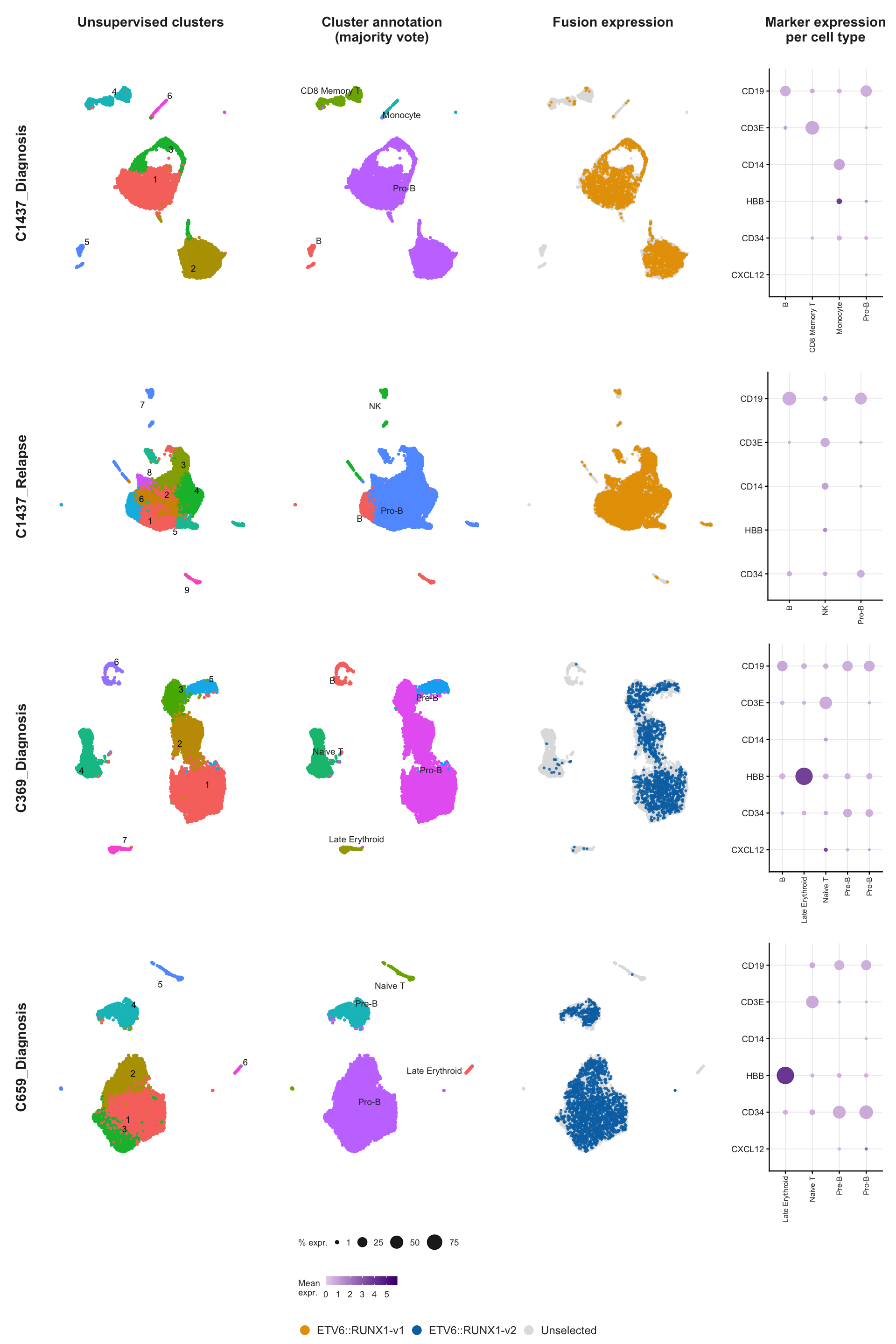

Past versions of fig-exp2-per-sample-fusion-umap-1.png

Version	Author	Date
74aa8d8	Jovana Maksimovic	2026-05-19
1b5bb97	Jovana Maksimovic	2026-05-11

supp_capture2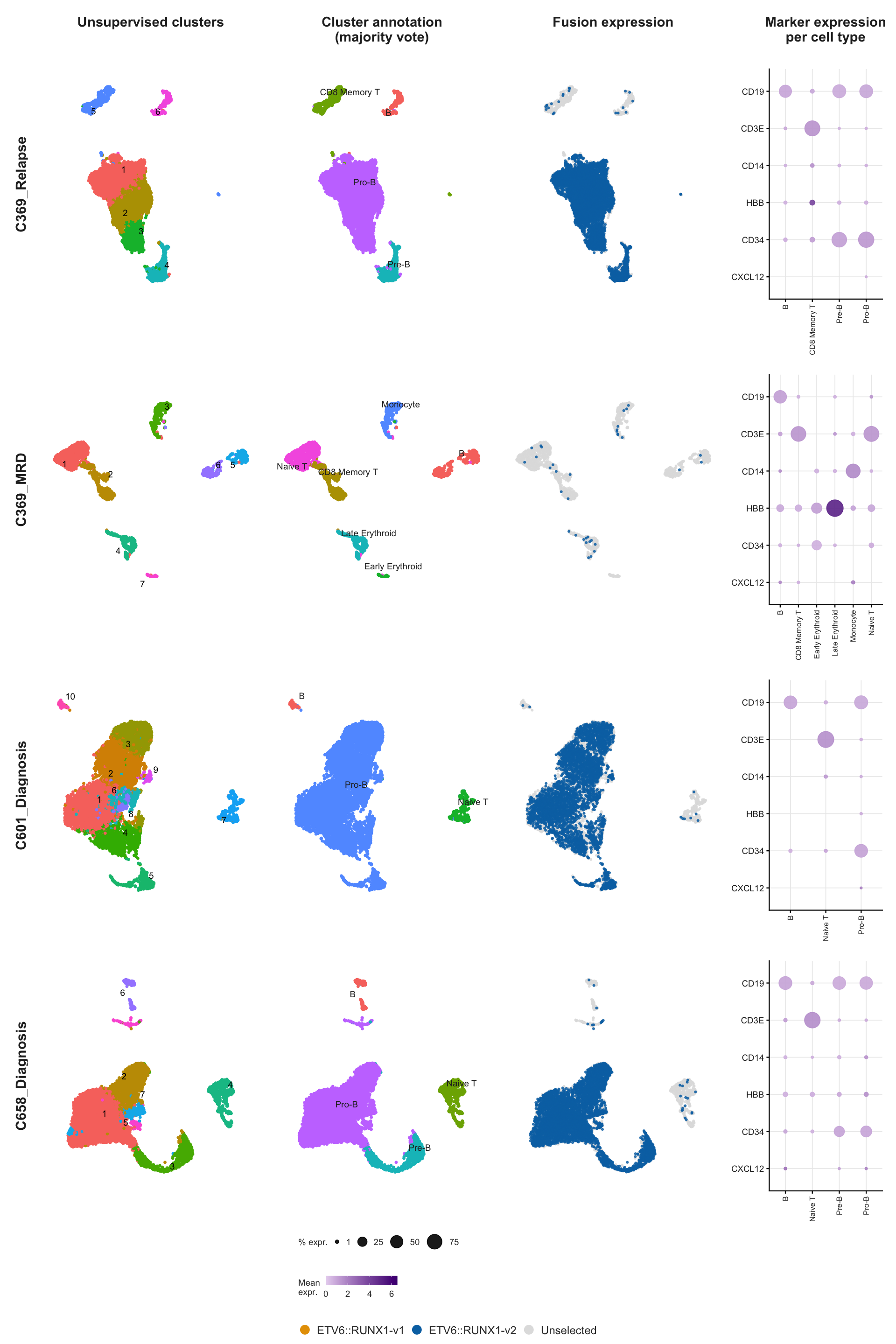

Past versions of fig-exp2-per-sample-fusion-umap-2.png

Version	Author	Date
1b5bb97	Jovana Maksimovic	2026-05-11

Expression of B-ALL marker DNTT is highly correlated with detected fusions.

lapply(seq_along(seu_lst), function(i){
  FeaturePlot(seu_lst[[i]], features = "DNTT") -> p1
  
  DimPlot(seu_lst[[i]], reduction = "umap", label = TRUE, repel = TRUE,
          label.size = 2.5, group.by = "SCT_snn_res.0.1", 
          cells.highlight = which(seu_lst[[i]]$patient_fusion != "not-detected"),
          sizes.highlight = 0.1) +
    NoLegend() -> p2
  
  (p1 / p2) + 
    plot_annotation(title = names(seu_lst)[i]) +
    theme(title = element_text(size = 10))
})

[[1]]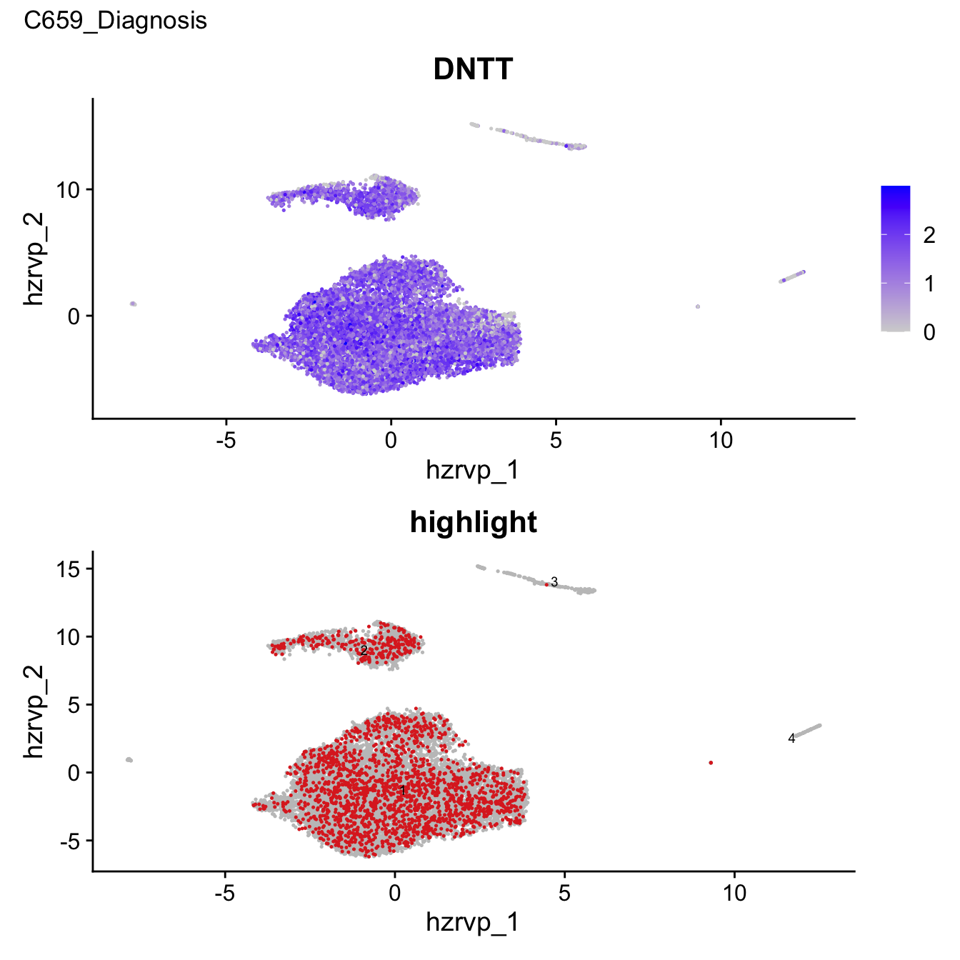

Past versions of plot-celltype-umap-1.png

Version	Author	Date
1b5bb97	Jovana Maksimovic	2026-05-11

[[2]]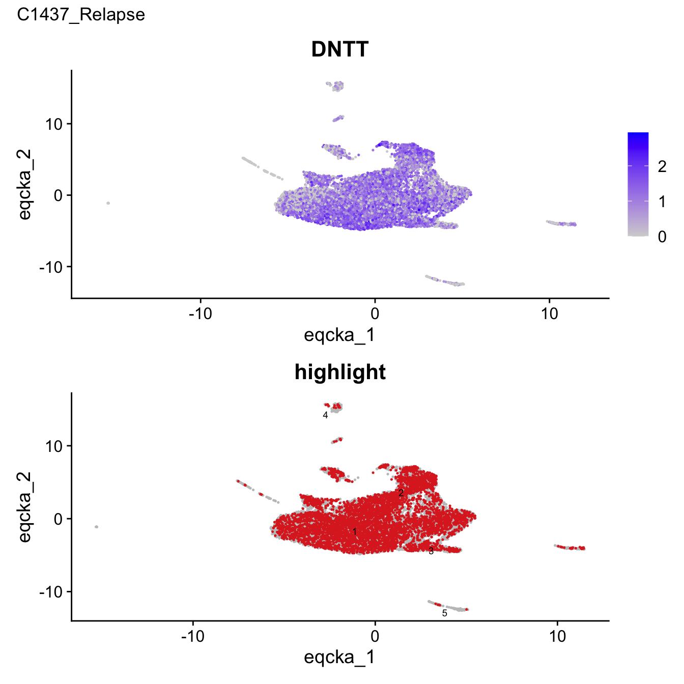

Past versions of plot-celltype-umap-2.png

Version	Author	Date
1b5bb97	Jovana Maksimovic	2026-05-11

[[3]]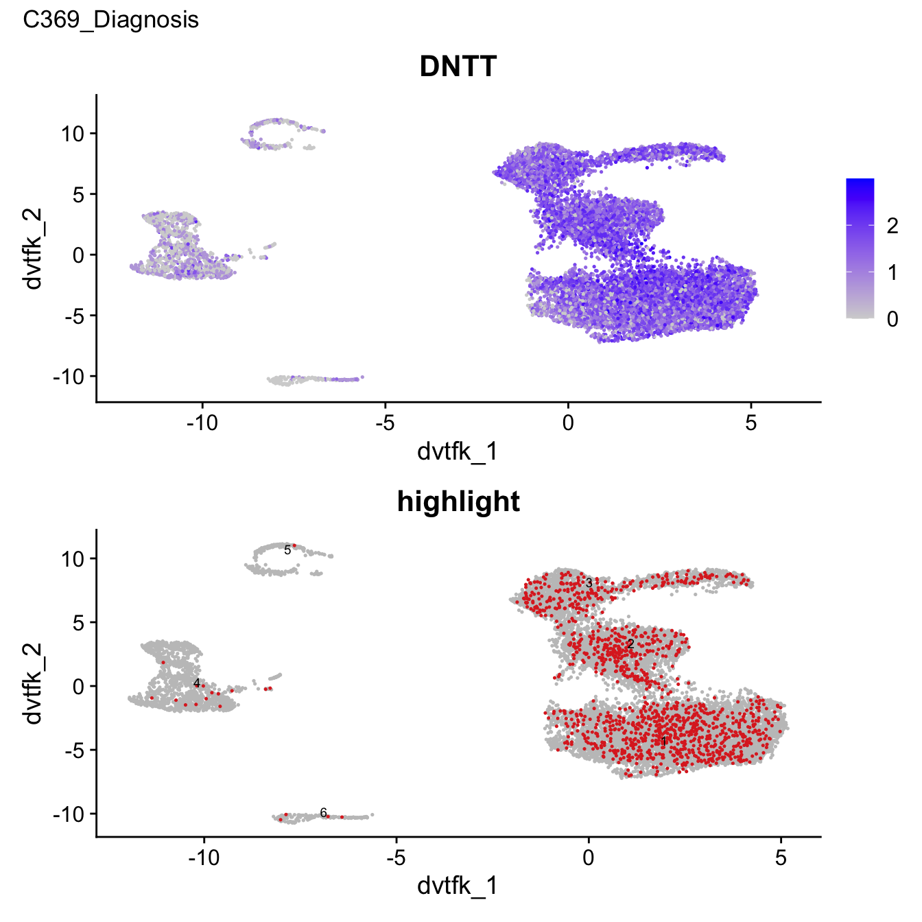

Past versions of plot-celltype-umap-3.png

Version	Author	Date
74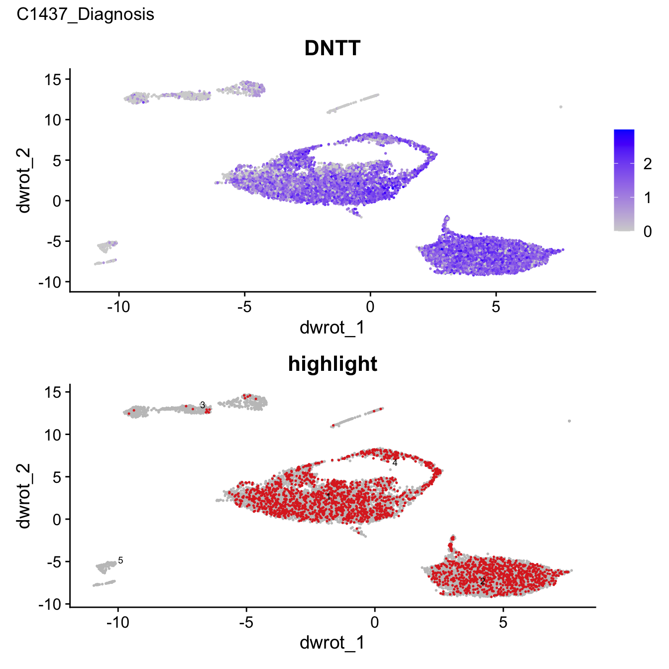aa8d8	Jovana Maksimovic	2026-05-19
1b5bb97	Jovana Maksimovic	2026-05-11

[[4]]

Past versions of plot-celltype-umap-4.png

Version	Author	Date
1b5bb97	Jovana Maksimovic	2026-05-11

[[5]]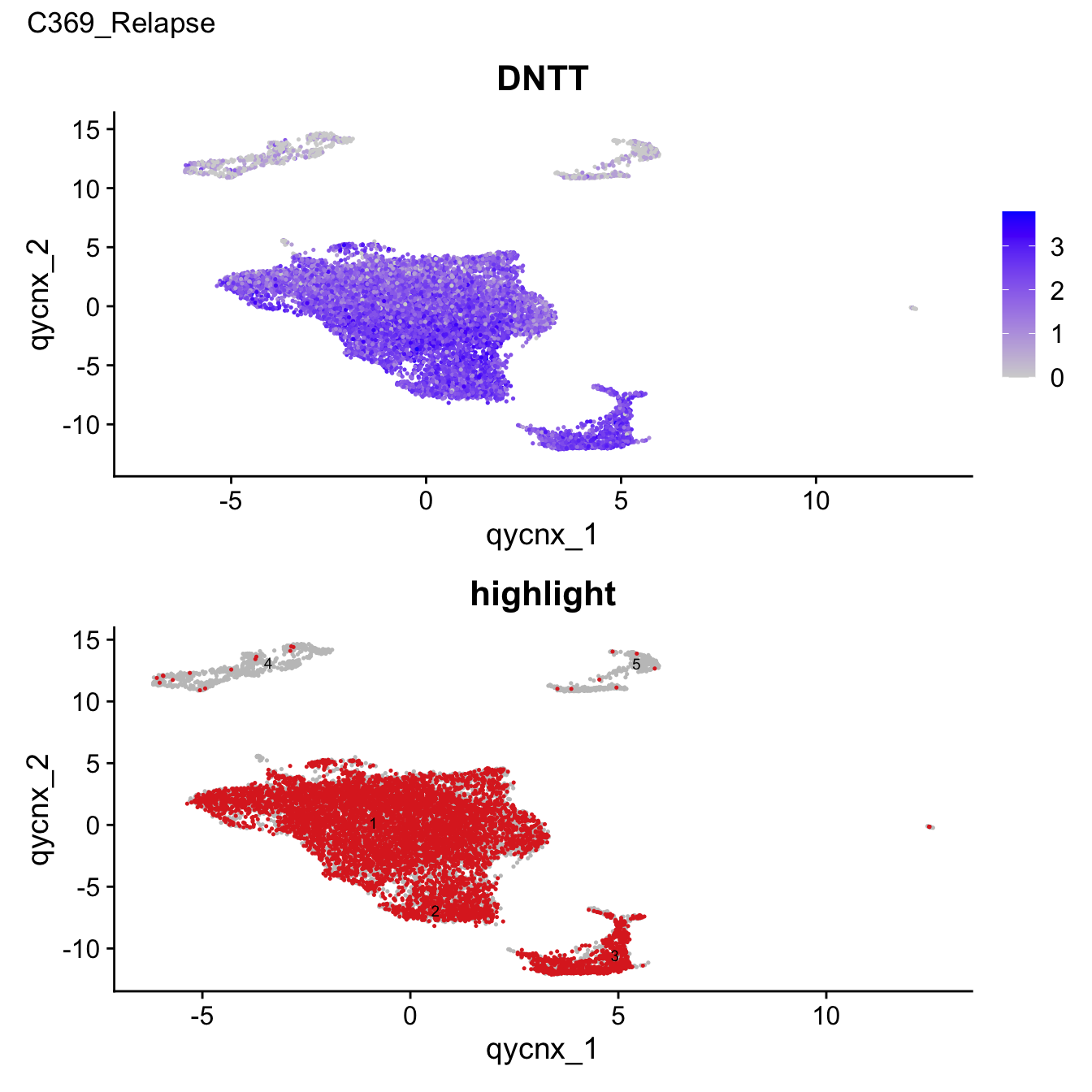

Past versions of plot-celltype-umap-5.png

Version	Author	Date
1b5bb97	Jovana Maksimovic	2026-05-11

[[6]]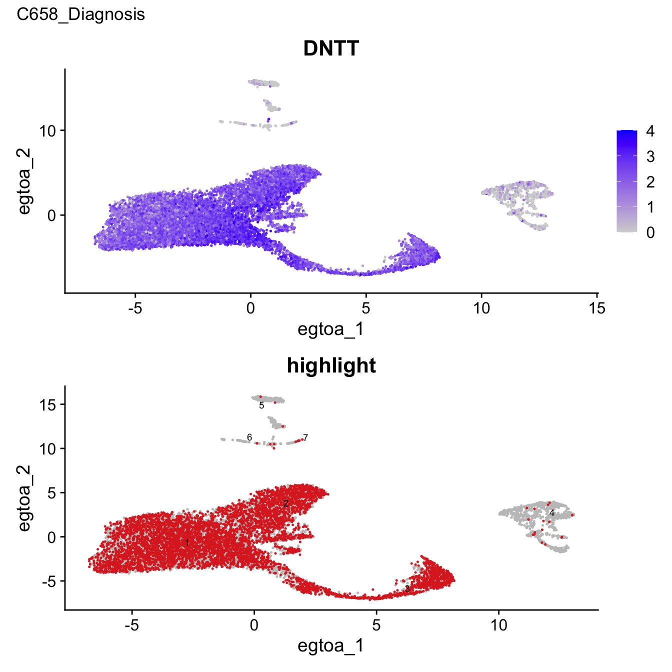

Past versions of plot-celltype-umap-6.png

Version	Author	Date
1b5bb97	Jovana Maksimovic	2026-05-11

[[7]]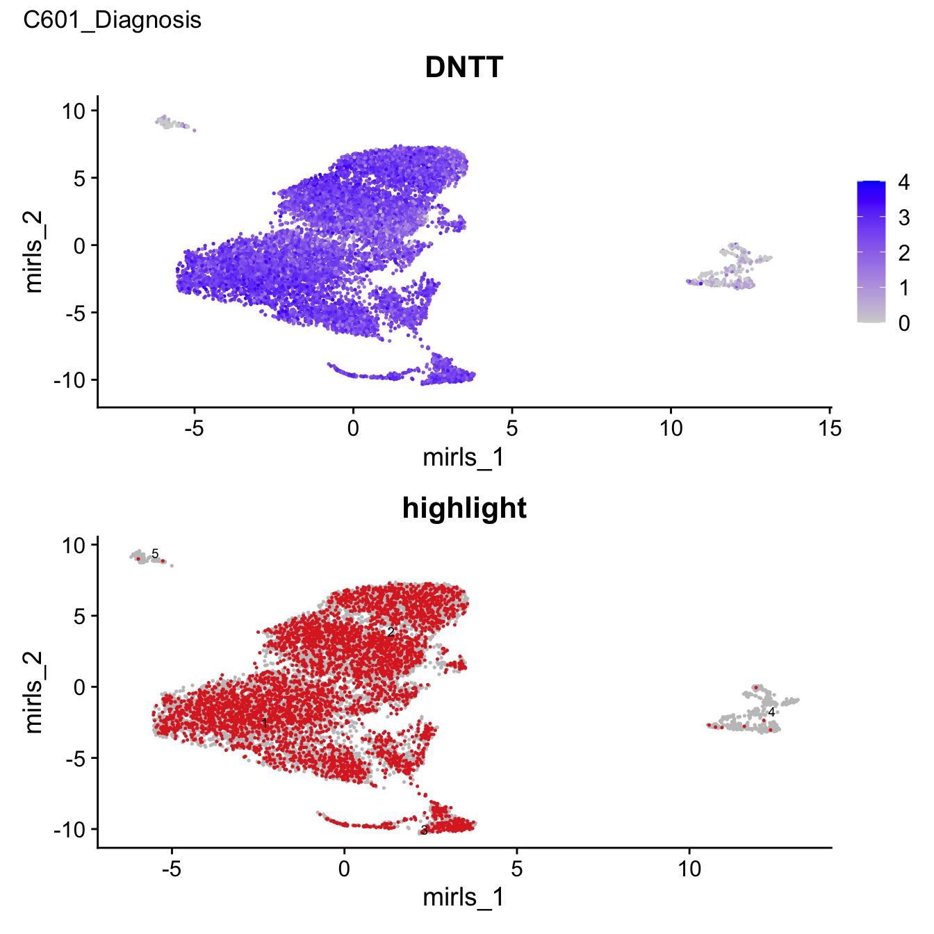

Past versions of plot-celltype-umap-7.png

Version	Author	Date
1b5bb97	Jovana Maksimovic	2026-05-11

[[8]]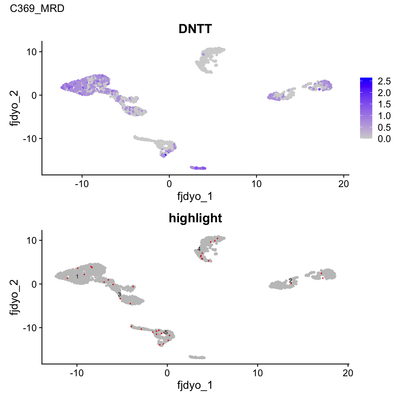

Past versions of plot-celltype-umap-8.png

Version	Author	Date
1b5bb97	Jovana Maksimovic	2026-05-11

C1437: diagnosis vs. relapse clone structure

Patient C1437 has samples from both diagnosis and relapse. Here the two timepoints are jointly clustered to identify diagnosis-specific and relapse-specific blast clones.

out <- here("data", "RDS", "ball_exp2_clustered_c1437.seu.rds")

if(!file.exists(out)) {
  
  seu_c1437 <- subset(seu, patient_timepoint %in% c("C1437_Diagnosis", "C1437_Relapse"))
  
  seu_c1437 <- SCTransform(seu_c1437, verbose = FALSE,
                           return.only.var.genes = TRUE)
  
  seu_c1437 <- RunPCA(seu_c1437, verbose = FALSE, npcs = 30, assay = "SCT")
  
  seu_c1437 <- RunUMAP(seu_c1437, dims = 1:30, reduction = "pca")
  
  seu_c1437 <- FindNeighbors(seu_c1437, reduction = "pca", dims = 1:30)
  
  seu_c1437 <- FindClusters(seu_c1437, resolution = seq(0.1, 1, by = 0.1),
                             algorithm = "Leiden")
  
  saveRDS(seu_c1437, file = out)
  fs::file_chmod(out, "664")
  try(fs::file_chown(out, group_id = "oshlack_lab"), silent = TRUE)
  
} else {
  seu_c1437 <- readRDS(out)
}

Select resolution

The lowest resolution (0.1) is probably sufficient for separating likely leukaemic clusters from clusters of other cells.

  clustree(seu_c1437, prefix = "SCT_snn_res.")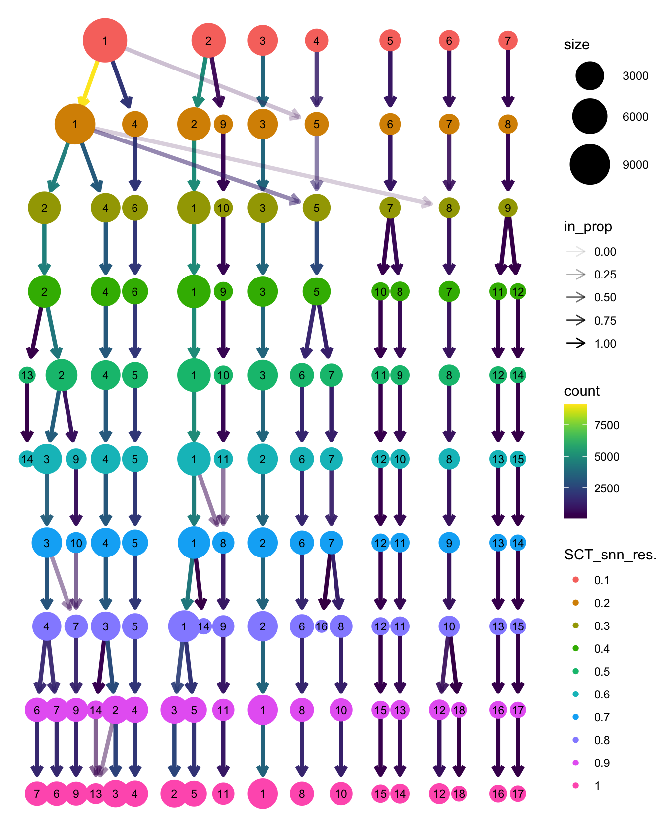

Past versions of c1437-clustree-1.png

Version	Author	Date
1b5bb97	Jovana Maksimovic	2026-05-11

p1 <- DimPlot(seu_c1437, group.by = "SCT_snn_res.0.3", 
              label = TRUE, repel = TRUE,
              label.size = 3) +
  ggtitle("Clusters (res 0.3)") +
  NoLegend()

p2 <- DimPlot(seu_c1437, group.by = "patient_timepoint",
              cols = c("C1437_Diagnosis" = "#56B4E9",
                       "C1437_Relapse"   = "#E69F00")) +
  ggtitle("Timepoint")

p3 <- DimPlot(seu_c1437, group.by = "predicted_CellType_Broad",
              label = TRUE, repel = TRUE,
              label.size = 3) +
  ggtitle("BoneMarrowMap annotation") +
  NoLegend()

p4 <- DimPlot(seu_c1437, group.by = "Phase",
              cols = c("G1"  = "#E69F00",
                       "G2M" = "#56B4E9",
                       "S"   = "#009E73")) +
  ggtitle("Cell cycle phase")

(p1 | p2) / (p3 | p4)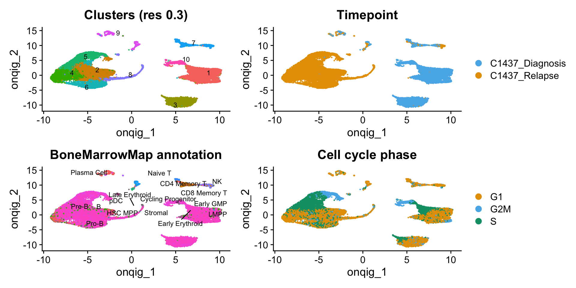

Past versions of c1437-clone-umap-1.png

Version	Author	Date
1b5bb97	Jovana Maksimovic	2026-05-11

Clusters are annotated as “Diagnosis clone”, “Relapse clone”, or “Normal BM” based on majority-vote cell type and the proportion of cells from each timepoint. This is an exploratory overview; the canonical publication C1437 figures (4F–4H) are assembled in B-ALL_exp2_c1437_clone_analysis.Rmd.

# Exploratory C1437 clone annotation — timepoint, clone identity, and fusion detection overview
# Step 1: majority vote cell type per cluster
blast_types <- c("Pro-B", "Pre-B", "Early Lymphoid")

cluster_meta <- seu_c1437@meta.data %>%
  group_by(SCT_snn_res.0.3) %>%
  summarise(
    majority_type    = names(which.max(table(predicted_CellType_Broad))),
    pct_diagnosis    = mean(patient_timepoint == "C1437_Diagnosis"),
    pct_relapse      = mean(patient_timepoint == "C1437_Relapse"),
    is_blast         = majority_type %in% blast_types,
    .groups          = "drop"
  ) %>%
  mutate(
    clone = dplyr::case_when(
      is_blast & pct_diagnosis >= 0.9 ~ "Diagnosis clone",
      is_blast & pct_relapse   >= 0.9 ~ "Relapse clone",
      !is_blast                       ~ "Normal BM",
      TRUE                            ~ "Mixed blast"   # safety catch
    )
  )

# Step 2: map back to cells
seu_c1437$clone <- cluster_meta$clone[
  match(seu_c1437$SCT_snn_res.0.3, cluster_meta$SCT_snn_res.0.3)
]

table(seu_c1437$clone)

Diagnosis clone       Normal BM   Relapse clone 
           9159            1482           13374 

clone_colours <- c(
  "Diagnosis clone" = "#0072B2",
  "Relapse clone"   = "#D55E00",
  "Normal BM"       = "#999999"
)

umap_arrow <- annotation_custom(
  grob = grid::grobTree(
    grid::segmentsGrob(
      x0 = 0.05, y0 = 0.05, x1 = 0.12, y1 = 0.05,
      arrow = grid::arrow(length = grid::unit(0.1, "cm"), type = "closed"),
      gp = grid::gpar(fill = "grey30", col = "grey30", lwd = 2)
    ),
    grid::segmentsGrob(
      x0 = 0.05, y0 = 0.05, x1 = 0.05, y1 = 0.12,
      arrow = grid::arrow(length = grid::unit(0.1, "cm"), type = "closed"),
      gp = grid::gpar(fill = "grey30", col = "grey30", lwd = 2)
    ),
    grid::textGrob(
      "UMAP", x = 0.085, y = 0.01,
      gp = grid::gpar(fontsize = 6, col = "grey30")
    )
  )
)

# Fusion highlight data
umap_coords_c1437 <- as.data.frame(Embeddings(seu_c1437, reduction = "umap"))
colnames(umap_coords_c1437) <- c("UMAP_1", "UMAP_2")
umap_coords_c1437$fusion_label <- dplyr::case_when(
  seu_c1437$patient_fusion == "ETV6-RUNX1-v1-fusion" ~ "ETV6::RUNX1-v1",
  TRUE                                                ~ "Unselected"
) %>% factor(levels = c("ETV6::RUNX1-v1", "Unselected"))

# Plot unselected first
umap_coords_c1437 <- umap_coords_c1437 %>%
  arrange(desc(fusion_label == "Unselected"))

seu_c1437$clone <- factor(seu_c1437$clone, 
                          levels = c("Diagnosis clone", 
                                     "Relapse clone", 
                                     "Normal BM"))

p1 <- DimPlot(seu_c1437, group.by = "patient_timepoint",
              cols = c("C1437_Diagnosis" = "#56B4E9",
                       "C1437_Relapse"   = "#E69F00"),
              pt.size = 0.3) +
  ggtitle("Timepoint") +
  theme_void() +
  theme(legend.position = "bottom") +
  umap_arrow

p2 <- DimPlot(seu_c1437, group.by = "clone",
              cols = clone_colours,
              pt.size = 0.3) +
  ggtitle("Clone") +
  theme_void() +
  theme(legend.position = "bottom") +
  scale_color_manual(values = clone_colours, drop = FALSE)

p3 <- ggplot(umap_coords_c1437, 
             aes(x = UMAP_1, y = UMAP_2, colour = fusion_label)) +
  geom_point(size = 0.3, alpha = 0.8) +
  scale_colour_manual(
    values = c(
      "ETV6::RUNX1-v1" = "#009E73",
      "Unselected"     = "grey88"
    ),
    drop = FALSE,
    guide = guide_legend(override.aes = list(size = 3))
  ) +
  ggtitle("Fusion detection") +
  labs(colour = NULL) +
  theme_void() +
  theme(legend.position = "bottom")

# Cleaner x labels and add percentage labels
seu_c1437@meta.data %>%
  group_by(patient_timepoint) %>%
  summarise(
    pct_fusion = mean(patient_fusion == "ETV6-RUNX1-v1-fusion") * 100,
    .groups = "drop"
  ) %>%
  mutate(label = paste0(round(pct_fusion, 1), "%"),
         patient_timepoint = gsub("C1437_", "", patient_timepoint)) %>%
  ggplot(aes(x = patient_timepoint, y = pct_fusion,
             fill = patient_timepoint)) +
  geom_col(width = 0.5) +
  geom_text(aes(label = label), vjust = -0.5, size = 2.5) +
  scale_fill_manual(values = c("Diagnosis" = "#0072B2",
                               "Relapse"   = "#D55E00")) +
  labs(x = NULL, y = "% fusion-positive cells") +
  theme_classic() +
  theme(legend.position = "none") -> p4

layout <- "
AAABBBCCC
AAABBBCCC
AAABBBCCC
##DDDDD##
##DDDDD##
"

(p1 + p2 + p3 + p4) +
  plot_layout(design = layout)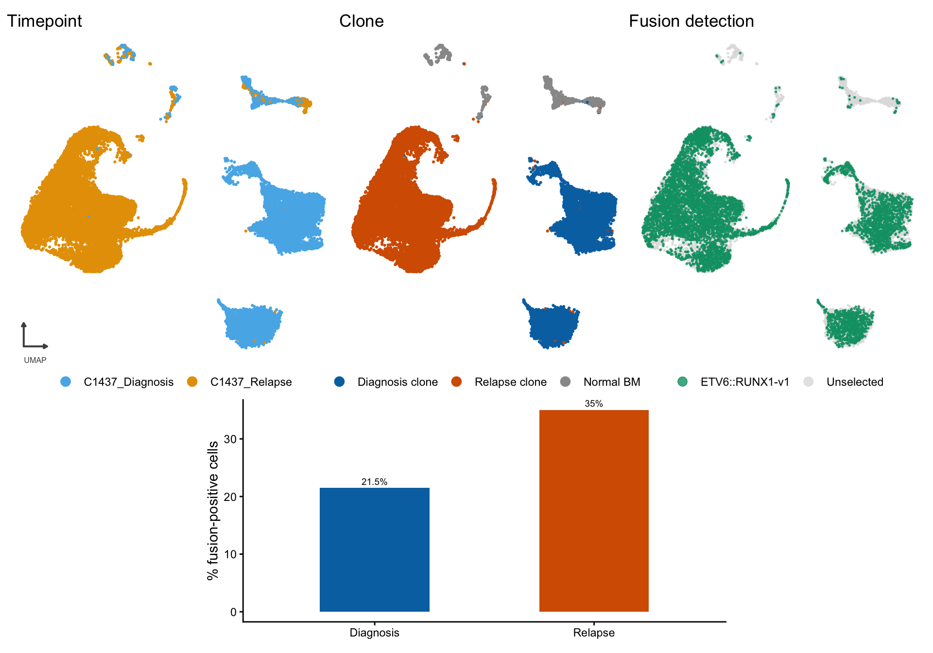

Past versions of fig-c1437-clone-annotation-1.png

Version	Author	Date
1b5bb97	Jovana Maksimovic	2026-05-11

# C1437 ETV6::RUNX1-v1 % fusion-positive cells at Diagnosis and Relapse
seu_c1437@meta.data %>%
  group_by(patient_timepoint) %>%
  summarise(
    total = n(),
    fusion_positive = sum(patient_fusion == "ETV6-RUNX1-v1-fusion"),
    pct_fusion = round(fusion_positive / total * 100, 1)
  )

# A tibble: 2 × 4
  patient_timepoint total fusion_positive pct_fusion
  <fct>             <int>           <int>      <dbl>
1 C1437_Diagnosis   10143            2182       21.5
2 C1437_Relapse     13872            4858       35  

seu_c1437@meta.data %>%
  group_by(patient_timepoint) %>%
  summarise(
    pct_fusion = mean(patient_fusion == "ETV6-RUNX1-v1-fusion") * 100,
    .groups = "drop"
  ) %>%
  ggplot(aes(x = patient_timepoint, y = pct_fusion,
             fill = patient_timepoint)) +
  geom_col(width = 0.6) +
  scale_fill_manual(values = c("C1437_Diagnosis" = "#56B4E9",
                                "C1437_Relapse"   = "#E69F00")) +
  labs(x = NULL, y = "% fusion-positive cells") +
  theme_classic() +
  theme(legend.position = "none")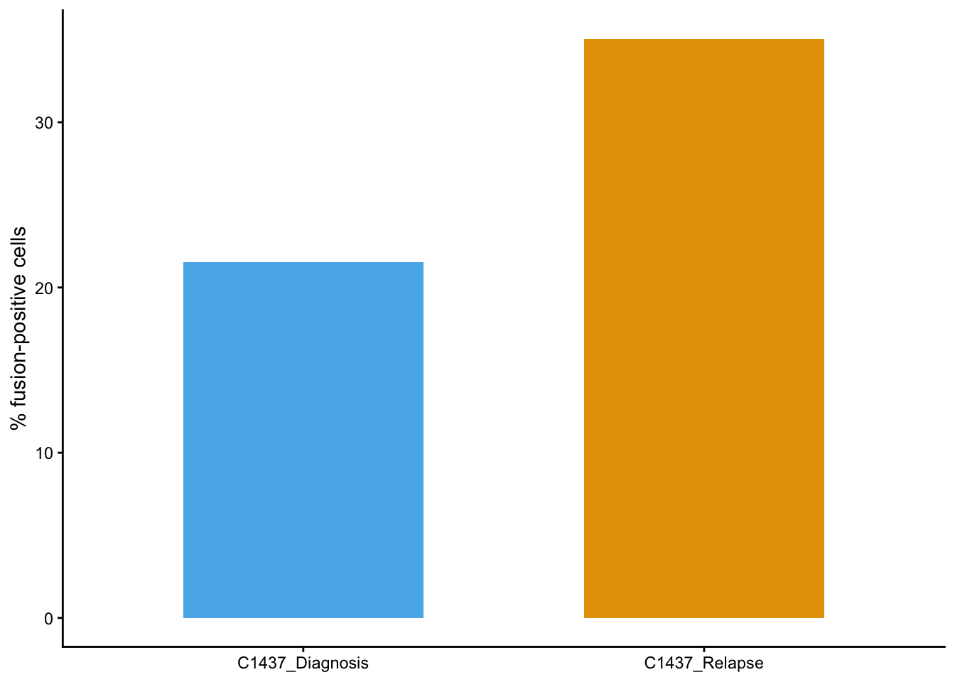

Past versions of fig-c1437-fusion-bar-1.png

Version	Author	Date
abab370	Jovana Maksimovic	2026-05-19

Session info

The analysis and this document were prepared using the following software (click triangle to expand)

sessioninfo::session_info()

─ Session info ───────────────────────────────────────────────────────────────
 setting  value
 version  R version 4.4.1 (2024-06-14)
 os       macOS 15.5
 system   aarch64, darwin20
 ui       X11
 language (EN)
 collate  en_US.UTF-8
 ctype    en_US.UTF-8
 tz       Australia/Melbourne
 date     2026-07-16
 pandoc   3.8.3 @ /Applications/RStudio.app/Contents/Resources/app/quarto/bin/tools/aarch64/ (via rmarkdown)
 quarto   1.9.38 @ /Applications/RStudio.app/Contents/Resources/app/quarto/bin/quarto

─ Packages ───────────────────────────────────────────────────────────────────
 ! package              * version   date (UTC) lib source
 P abind                  1.4-8     2024-09-12 [?] CRAN (R 4.4.1)
 P backports              1.5.0     2024-05-23 [?] CRAN (R 4.4.1)
 P beeswarm               0.4.0     2021-06-01 [?] CRAN (R 4.4.1)
 P Biobase                2.66.0    2024-11-08 [?] Bioconduc~
 P BiocGenerics           0.52.0    2024-11-08 [?] Bioconduc~
 P BiocManager            1.30.27   2025-11-14 [?] CRAN (R 4.4.3)
 P bslib                  0.9.0     2025-01-30 [?] CRAN (R 4.4.1)
 P cachem                 1.1.0     2024-05-16 [?] CRAN (R 4.4.1)
 P callr                  3.7.6     2024-03-25 [?] CRAN (R 4.4.0)
 P checkmate              2.3.2     2024-07-29 [?] CRAN (R 4.4.0)
 P cli                    3.6.5     2025-04-23 [?] CRAN (R 4.4.1)
 P cluster                2.1.6     2023-12-01 [?] CRAN (R 4.4.1)
 P clustree             * 0.5.1     2023-11-05 [?] CRAN (R 4.4.0)
 P codetools              0.2-20    2024-03-31 [?] CRAN (R 4.4.1)
 P colorspace             2.1-1     2024-07-26 [?] CRAN (R 4.4.1)
 P cowplot                1.1.3     2024-01-22 [?] CRAN (R 4.4.0)
 P crayon                 1.5.3     2024-06-20 [?] CRAN (R 4.4.1)
 P data.table             1.18.2.1  2026-01-27 [?] CRAN (R 4.4.3)
 P DelayedArray           0.32.0    2024-11-08 [?] Bioconduc~
 P deldir                 2.0-4     2024-02-28 [?] CRAN (R 4.4.1)
 P digest                 0.6.37    2024-08-19 [?] CRAN (R 4.4.1)
 P dotCall64              1.2       2024-10-04 [?] CRAN (R 4.4.1)
 P dplyr                * 1.1.4     2023-11-17 [?] CRAN (R 4.4.0)
 P evaluate               1.0.3     2025-01-10 [?] CRAN (R 4.4.1)
 P farver                 2.1.2     2024-05-13 [?] CRAN (R 4.4.1)
 P fastDummies            1.7.5     2025-01-20 [?] CRAN (R 4.4.1)
 P fastmap                1.2.0     2024-05-15 [?] CRAN (R 4.4.1)
 P fitdistrplus           1.2-2     2025-01-07 [?] CRAN (R 4.4.1)
 P forcats              * 1.0.0     2023-01-29 [?] CRAN (R 4.4.0)
 P fs                     1.6.6     2025-04-12 [?] CRAN (R 4.4.1)
 P future                 1.49.0    2025-05-09 [?] CRAN (R 4.4.1)
 P future.apply           1.11.3    2024-10-27 [?] CRAN (R 4.4.1)
 P generics               0.1.4     2025-05-09 [?] CRAN (R 4.4.1)
 P GenomeInfoDb           1.42.3    2025-01-27 [?] Bioconduc~
 P GenomeInfoDbData       1.2.13    2025-05-28 [?] Bioconductor
 P GenomicRanges          1.58.0    2024-11-08 [?] Bioconduc~
 P getPass                0.2-4     2023-12-10 [?] CRAN (R 4.4.1)
 P ggbeeswarm             0.7.2     2023-04-29 [?] CRAN (R 4.4.0)
 P ggforce                0.4.2     2024-02-19 [?] CRAN (R 4.4.0)
 P ggplot2              * 4.0.2     2026-02-03 [?] CRAN (R 4.4.3)
 P ggraph               * 2.2.1     2024-03-07 [?] CRAN (R 4.4.0)
 P ggrastr                1.0.2     2023-06-01 [?] CRAN (R 4.4.0)
 P ggrepel              * 0.9.6     2024-09-07 [?] CRAN (R 4.4.1)
 P ggridges               0.5.6     2024-01-23 [?] CRAN (R 4.4.0)
 P git2r                  0.36.2    2025-03-29 [?] CRAN (R 4.4.1)
 P glmGamPoi            * 1.18.0    2024-11-08 [?] Bioconduc~
 P globals                0.18.0    2025-05-08 [?] CRAN (R 4.4.1)
 P glue                 * 1.8.0     2024-09-30 [?] CRAN (R 4.4.1)
 P goftest                1.2-3     2021-10-07 [?] CRAN (R 4.4.1)
 P graphlayouts           1.2.2     2025-01-23 [?] CRAN (R 4.4.1)
 P gridExtra              2.3       2017-09-09 [?] CRAN (R 4.4.1)
 P gtable                 0.3.6     2024-10-25 [?] CRAN (R 4.4.1)
 P here                 * 1.0.1     2020-12-13 [?] CRAN (R 4.4.1)
 P hms                    1.1.3     2023-03-21 [?] CRAN (R 4.4.0)
 P htmltools              0.5.8.1   2024-04-04 [?] CRAN (R 4.4.1)
 P htmlwidgets            1.6.4     2023-12-06 [?] CRAN (R 4.4.0)
 P httpuv                 1.6.16    2025-04-16 [?] CRAN (R 4.4.1)
 P httr                   1.4.7     2023-08-15 [?] CRAN (R 4.4.0)
 P ica                    1.0-3     2022-07-08 [?] CRAN (R 4.4.1)
 P igraph                 2.1.4     2025-01-23 [?] CRAN (R 4.4.1)
 P IRanges                2.40.1    2024-12-05 [?] Bioconduc~
 P irlba                  2.3.5.1   2022-10-03 [?] CRAN (R 4.4.0)
 P jquerylib              0.1.4     2021-04-26 [?] CRAN (R 4.4.0)
 P jsonlite               2.0.0     2025-03-27 [?] CRAN (R 4.4.1)
 P KernSmooth             2.23-24   2024-05-17 [?] CRAN (R 4.4.1)
 P knitr                  1.50      2025-03-16 [?] CRAN (R 4.4.1)
 P labeling               0.4.3     2023-08-29 [?] CRAN (R 4.4.1)
 P later                  1.4.2     2025-04-08 [?] CRAN (R 4.4.1)
 P lattice                0.22-6    2024-03-20 [?] CRAN (R 4.4.1)
 P lazyeval               0.2.2     2019-03-15 [?] CRAN (R 4.4.1)
 P lifecycle              1.0.4     2023-11-07 [?] CRAN (R 4.4.1)
 P listenv                0.9.1     2024-01-29 [?] CRAN (R 4.4.1)
 P lmtest                 0.9-40    2022-03-21 [?] CRAN (R 4.4.1)
 P lubridate            * 1.9.4     2024-12-08 [?] CRAN (R 4.4.1)
 P magrittr               2.0.3     2022-03-30 [?] CRAN (R 4.4.1)
 P MASS                   7.3-60.2  2024-04-26 [?] CRAN (R 4.4.1)
 P Matrix                 1.7-0     2024-04-26 [?] CRAN (R 4.4.1)
 P MatrixGenerics         1.18.1    2025-01-09 [?] Bioconduc~
 P matrixStats            1.5.0     2025-01-07 [?] CRAN (R 4.4.1)
 P memoise                2.0.1     2021-11-26 [?] CRAN (R 4.4.0)
 P mime                   0.13      2025-03-17 [?] CRAN (R 4.4.1)
 P miniUI                 0.1.2     2025-04-17 [?] CRAN (R 4.4.1)
 P nlme                   3.1-164   2023-11-27 [?] CRAN (R 4.4.1)
 P paletteer              1.6.0     2024-01-21 [?] CRAN (R 4.4.0)
 P parallelly             1.45.0    2025-06-02 [?] CRAN (R 4.4.1)
 P patchwork            * 1.3.0     2024-09-16 [?] CRAN (R 4.4.1)
 P pbapply                1.7-4     2025-07-20 [?] CRAN (R 4.4.1)
 P pillar                 1.10.2    2025-04-05 [?] CRAN (R 4.4.1)
 P pkgconfig              2.0.3     2019-09-22 [?] CRAN (R 4.4.1)
 P plotly                 4.10.4    2024-01-13 [?] CRAN (R 4.4.0)
 P plyr                   1.8.9     2023-10-02 [?] CRAN (R 4.4.1)
 P png                    0.1-8     2022-11-29 [?] CRAN (R 4.4.1)
 P polyclip               1.10-7    2024-07-23 [?] CRAN (R 4.4.1)
 P prismatic              1.1.2     2024-04-10 [?] CRAN (R 4.4.1)
 P processx               3.8.6     2025-02-21 [?] CRAN (R 4.4.1)
 P progressr              0.15.1    2024-11-22 [?] CRAN (R 4.4.1)
 P promises               1.3.3     2025-05-29 [?] CRAN (R 4.4.1)
 P ps                     1.9.1     2025-04-12 [?] CRAN (R 4.4.1)
 P purrr                * 1.0.4     2025-02-05 [?] CRAN (R 4.4.1)
 P R6                     2.6.1     2025-02-15 [?] CRAN (R 4.4.1)
 P RANN                   2.6.2     2024-08-25 [?] CRAN (R 4.4.1)
 P RColorBrewer           1.1-3     2022-04-03 [?] CRAN (R 4.4.1)
 P Rcpp                   1.1.1-1.1 2026-04-24 [?] CRAN (R 4.4.1)
 P RcppAnnoy              0.0.22    2024-01-23 [?] CRAN (R 4.4.1)
 P RcppHNSW               0.6.0     2024-02-04 [?] CRAN (R 4.4.1)
 P readr                * 2.1.5     2024-01-10 [?] CRAN (R 4.4.0)
 P rematch2               2.1.2     2020-05-01 [?] CRAN (R 4.4.0)
   renv                   1.1.4     2025-03-20 [1] CRAN (R 4.4.1)
 P reshape2               1.4.4     2020-04-09 [?] CRAN (R 4.4.0)
 P reticulate             1.42.0    2025-03-25 [?] CRAN (R 4.4.1)
 P rlang                  1.1.6     2025-04-11 [?] CRAN (R 4.4.1)
 P rmarkdown              2.29      2024-11-04 [?] CRAN (R 4.4.1)
 P ROCR                   1.0-11    2020-05-02 [?] CRAN (R 4.4.0)
 P rprojroot              2.0.4     2023-11-05 [?] CRAN (R 4.4.1)
 P RSpectra               0.16-2    2024-07-18 [?] CRAN (R 4.4.0)
 P rstudioapi             0.17.1    2024-10-22 [?] CRAN (R 4.4.1)
 P Rtsne                  0.17      2023-12-07 [?] CRAN (R 4.4.1)
 P S4Arrays               1.6.0     2024-11-08 [?] Bioconduc~
 P S4Vectors              0.44.0    2024-11-08 [?] Bioconduc~
 P S7                     0.2.0     2024-11-07 [?] CRAN (R 4.4.1)
 P sass                   0.4.10    2025-04-11 [?] CRAN (R 4.4.1)
 P scales               * 1.4.0     2025-04-24 [?] CRAN (R 4.4.1)
 P scattermore            1.2       2023-06-12 [?] CRAN (R 4.4.0)
 P sctransform            0.4.2     2025-04-30 [?] CRAN (R 4.4.1)
 P sessioninfo            1.2.3     2025-02-05 [?] CRAN (R 4.4.1)
 P Seurat               * 5.3.0     2025-04-23 [?] CRAN (R 4.4.1)
 P SeuratObject         * 5.1.0     2025-04-22 [?] CRAN (R 4.4.1)
 P shiny                  1.10.0    2024-12-14 [?] CRAN (R 4.4.1)
 P sp                   * 2.2-0     2025-02-01 [?] CRAN (R 4.4.1)
 P spam                   2.11-1    2025-01-20 [?] CRAN (R 4.4.1)
 P SparseArray            1.6.2     2025-02-20 [?] Bioconduc~
 P spatstat.data          3.1-6     2025-03-17 [?] CRAN (R 4.4.1)
 P spatstat.explore       3.4-3     2025-05-21 [?] CRAN (R 4.4.1)
 P spatstat.geom          3.4-1     2025-05-20 [?] CRAN (R 4.4.1)
 P spatstat.random        3.4-1     2025-05-20 [?] CRAN (R 4.4.1)
 P spatstat.sparse        3.1-0     2024-06-21 [?] CRAN (R 4.4.0)
 P spatstat.univar        3.1-3     2025-05-08 [?] CRAN (R 4.4.1)
 P spatstat.utils         3.1-4     2025-05-15 [?] CRAN (R 4.4.1)
 P stringi                1.8.7     2025-03-27 [?] CRAN (R 4.4.1)
 P stringr              * 1.6.0     2025-11-04 [?] CRAN (R 4.4.1)
 P SummarizedExperiment   1.36.0    2024-11-08 [?] Bioconduc~
 P survival               3.6-4     2024-04-24 [?] CRAN (R 4.4.1)
 P tensor                 1.5       2012-05-05 [?] CRAN (R 4.4.1)
 P tibble               * 3.2.1     2023-03-20 [?] CRAN (R 4.4.0)
 P tidygraph              1.3.1     2024-01-30 [?] CRAN (R 4.4.0)
 P tidyr                * 1.3.1     2024-01-24 [?] CRAN (R 4.4.1)
 P tidyselect             1.2.1     2024-03-11 [?] CRAN (R 4.4.0)
 P tidyverse            * 2.0.0     2023-02-22 [?] CRAN (R 4.4.0)
 P timechange             0.3.0     2024-01-18 [?] CRAN (R 4.4.1)
 P tweenr                 2.0.3     2024-02-26 [?] CRAN (R 4.4.0)
 P tzdb                   0.5.0     2025-03-15 [?] CRAN (R 4.4.1)
 P UCSC.utils             1.2.0     2024-11-08 [?] Bioconduc~
 P utf8                   1.2.5     2025-05-01 [?] CRAN (R 4.4.1)
 P uwot                   0.2.3     2025-02-24 [?] CRAN (R 4.4.1)
 P vctrs                  0.6.5     2023-12-01 [?] CRAN (R 4.4.0)
 P vipor                  0.4.7     2023-12-18 [?] CRAN (R 4.4.1)
 P viridis                0.6.5     2024-01-29 [?] CRAN (R 4.4.0)
 P viridisLite            0.4.2     2023-05-02 [?] CRAN (R 4.4.1)
 P whisker                0.4.1     2022-12-05 [?] CRAN (R 4.4.1)
 P withr                  3.0.2     2024-10-28 [?] CRAN (R 4.4.1)
 P workflowr            * 1.7.1     2023-08-23 [?] CRAN (R 4.4.0)
 P xfun                   0.56      2026-01-18 [?] CRAN (R 4.4.3)
 P xtable                 1.8-4     2019-04-21 [?] CRAN (R 4.4.1)
 P XVector                0.46.0    2024-11-08 [?] Bioconduc~
 P yaml                   2.3.10    2024-07-26 [?] CRAN (R 4.4.1)
 P zlibbioc               1.52.0    2024-11-08 [?] Bioconduc~
 P zoo                    1.8-14    2025-04-10 [?] CRAN (R 4.4.1)

 [1] /Users/maksimovicjovana/projects/active/flex-fusion-probes/renv/library/macos/R-4.4/aarch64-apple-darwin20
 [2] /Users/maksimovicjovana/Library/Caches/org.R-project.R/R/renv/sandbox/macos/R-4.4/aarch64-apple-darwin20/f7156815

 * ── Packages attached to the search path.
 P ── Loaded and on-disk path mismatch.

──────────────────────────────────────────────────────────────────────────────

Session information

sessionInfo()

R version 4.4.1 (2024-06-14)
Platform: aarch64-apple-darwin20
Running under: macOS 15.5

Matrix products: default
BLAS:   /Library/Frameworks/R.framework/Versions/4.4-arm64/Resources/lib/libRblas.0.dylib 
LAPACK: /Library/Frameworks/R.framework/Versions/4.4-arm64/Resources/lib/libRlapack.dylib;  LAPACK version 3.12.0

locale:
[1] en_US.UTF-8/en_US.UTF-8/en_US.UTF-8/C/en_US.UTF-8/en_US.UTF-8

time zone: Australia/Melbourne
tzcode source: internal

attached base packages:
[1] stats     graphics  grDevices datasets  utils     methods   base     

other attached packages:
 [1] ggrepel_0.9.6      glmGamPoi_1.18.0   clustree_0.5.1     ggraph_2.2.1      
 [5] patchwork_1.3.0    scales_1.4.0       Seurat_5.3.0       SeuratObject_5.1.0
 [9] sp_2.2-0           glue_1.8.0         here_1.0.1         lubridate_1.9.4   
[13] forcats_1.0.0      stringr_1.6.0      dplyr_1.1.4        purrr_1.0.4       
[17] readr_2.1.5        tidyr_1.3.1        tibble_3.2.1       ggplot2_4.0.2     
[21] tidyverse_2.0.0    workflowr_1.7.1   

loaded via a namespace (and not attached):
  [1] RcppAnnoy_0.0.22            splines_4.4.1              
  [3] later_1.4.2                 prismatic_1.1.2            
  [5] polyclip_1.10-7             fastDummies_1.7.5          
  [7] lifecycle_1.0.4             rprojroot_2.0.4            
  [9] globals_0.18.0              processx_3.8.6             
 [11] lattice_0.22-6              MASS_7.3-60.2              
 [13] backports_1.5.0             magrittr_2.0.3             
 [15] plotly_4.10.4               sass_0.4.10                
 [17] rmarkdown_2.29              jquerylib_0.1.4            
 [19] yaml_2.3.10                 httpuv_1.6.16              
 [21] sctransform_0.4.2           spam_2.11-1                
 [23] sessioninfo_1.2.3           spatstat.sparse_3.1-0      
 [25] reticulate_1.42.0           cowplot_1.1.3              
 [27] pbapply_1.7-4               RColorBrewer_1.1-3         
 [29] abind_1.4-8                 zlibbioc_1.52.0            
 [31] Rtsne_0.17                  GenomicRanges_1.58.0       
 [33] BiocGenerics_0.52.0         tweenr_2.0.3               
 [35] git2r_0.36.2                GenomeInfoDbData_1.2.13    
 [37] IRanges_2.40.1              S4Vectors_0.44.0           
 [39] irlba_2.3.5.1               listenv_0.9.1              
 [41] spatstat.utils_3.1-4        goftest_1.2-3              
 [43] RSpectra_0.16-2             spatstat.random_3.4-1      
 [45] fitdistrplus_1.2-2          parallelly_1.45.0          
 [47] codetools_0.2-20            DelayedArray_0.32.0        
 [49] ggforce_0.4.2               tidyselect_1.2.1           
 [51] UCSC.utils_1.2.0            farver_2.1.2               
 [53] viridis_0.6.5               matrixStats_1.5.0          
 [55] stats4_4.4.1                spatstat.explore_3.4-3     
 [57] jsonlite_2.0.0              tidygraph_1.3.1            
 [59] progressr_0.15.1            ggridges_0.5.6             
 [61] survival_3.6-4              tools_4.4.1                
 [63] ica_1.0-3                   Rcpp_1.1.1-1.1             
 [65] SparseArray_1.6.2           gridExtra_2.3              
 [67] xfun_0.56                   MatrixGenerics_1.18.1      
 [69] GenomeInfoDb_1.42.3         withr_3.0.2                
 [71] BiocManager_1.30.27         fastmap_1.2.0              
 [73] callr_3.7.6                 digest_0.6.37              
 [75] timechange_0.3.0            R6_2.6.1                   
 [77] mime_0.13                   colorspace_2.1-1           
 [79] scattermore_1.2             tensor_1.5                 
 [81] spatstat.data_3.1-6         utf8_1.2.5                 
 [83] generics_0.1.4              renv_1.1.4                 
 [85] data.table_1.18.2.1         graphlayouts_1.2.2         
 [87] httr_1.4.7                  htmlwidgets_1.6.4          
 [89] S4Arrays_1.6.0              whisker_0.4.1              
 [91] uwot_0.2.3                  pkgconfig_2.0.3            
 [93] gtable_0.3.6                lmtest_0.9-40              
 [95] S7_0.2.0                    XVector_0.46.0             
 [97] htmltools_0.5.8.1           dotCall64_1.2              
 [99] Biobase_2.66.0              png_0.1-8                  
[101] spatstat.univar_3.1-3       knitr_1.50                 
[103] rstudioapi_0.17.1           tzdb_0.5.0                 
[105] reshape2_1.4.4              checkmate_2.3.2            
[107] nlme_3.1-164                cachem_1.1.0               
[109] zoo_1.8-14                  KernSmooth_2.23-24         
[111] vipor_0.4.7                 parallel_4.4.1             
[113] miniUI_0.1.2                ggrastr_1.0.2              
[115] pillar_1.10.2               grid_4.4.1                 
[117] vctrs_0.6.5                 RANN_2.6.2                 
[119] promises_1.3.3              xtable_1.8-4               
[121] cluster_2.1.6               beeswarm_0.4.0             
[123] paletteer_1.6.0             evaluate_1.0.3             
[125] cli_3.6.5                   compiler_4.4.1             
[127] rlang_1.1.6                 crayon_1.5.3               
[129] future.apply_1.11.3         labeling_0.4.3             
[131] rematch2_2.1.2              ps_1.9.1                   
[133] ggbeeswarm_0.7.2            getPass_0.2-4              
[135] plyr_1.8.9                  fs_1.6.6                   
[137] stringi_1.8.7               viridisLite_0.4.2          
[139] deldir_2.0-4                lazyeval_0.2.2             
[141] spatstat.geom_3.4-1         Matrix_1.7-0               
[143] RcppHNSW_0.6.0              hms_1.1.3                  
[145] future_1.49.0               shiny_1.10.0               
[147] SummarizedExperiment_1.36.0 ROCR_1.0-11                
[149] igraph_2.1.4                memoise_2.0.1              
[151] bslib_0.9.0