B-ALL Experiment 2: Joint Clustering
Joint Leiden clustering, normal BM re-embedding, and Figures 4B–C assembly
Jovana Maksimovic
July 16, 2026
Last updated: 2026-07-16
Checks: 7 0
Knit directory: flex-fusion-probes/
This reproducible R Markdown analysis was created with workflowr (version 1.7.1). The Checks tab describes the reproducibility checks that were applied when the results were created. The Past versions tab lists the development history.
Great! Since the R Markdown file has been committed to the Git repository, you know the exact version of the code that produced these results.
Great job! The global environment was empty. Objects defined in the global environment can affect the analysis in your R Markdown file in unknown ways. For reproduciblity it’s best to always run the code in an empty environment.
The command set.seed(20240925) was run prior to running
the code in the R Markdown file. Setting a seed ensures that any results
that rely on randomness, e.g. subsampling or permutations, are
reproducible.
Great job! Recording the operating system, R version, and package versions is critical for reproducibility.
Nice! There were no cached chunks for this analysis, so you can be confident that you successfully produced the results during this run.
Great job! Using relative paths to the files within your workflowr project makes it easier to run your code on other machines.
Great! You are using Git for version control. Tracking code development and connecting the code version to the results is critical for reproducibility.
The results in this page were generated with repository version 8fa721b. See the Past versions tab to see a history of the changes made to the R Markdown and HTML files.
Note that you need to be careful to ensure that all relevant files for
the analysis have been committed to Git prior to generating the results
(you can use wflow_publish or
wflow_git_commit). workflowr only checks the R Markdown
file, but you know if there are other scripts or data files that it
depends on. Below is the status of the Git repository when the results
were generated:
Ignored files:
    Ignored:    .DS_Store
    Ignored:    .Rhistory
    Ignored:    .Rproj.user/
    Ignored:    analysis/.gitignore
    Ignored:    analysis/obsolete/B-ALL_nonblast_fusion_analysis_cache/
    Ignored:    analysis/projectionFigures/
    Ignored:    code/files/
    Ignored:    data/.DS_Store
    Ignored:    data/BoneMarrowMap/
    Ignored:    data/BoneMarrowMapBoneMarrowMap_SymphonyReference.rds
    Ignored:    data/BoneMarrowMapBoneMarrowMap_uwot_model.uwot
    Ignored:    data/CAPTURE-1-POOL-FLEX/
    Ignored:    data/CAPTURE-2-POOL-FLEX/
    Ignored:    data/Pool-240917-FLEX/
    Ignored:    data/RDS/
    Ignored:    data/Run_1_and_Run_2/
    Ignored:    data/Run_2/
    Ignored:    logs/
    Ignored:    output/
    Ignored:    projectionFigures/
    Ignored:    renv/library/
    Ignored:    renv/staging/

Untracked files:
    Untracked:  CLAUDE.md
    Untracked:  analysis/B-ALL_exp2_nonblast_fusion_analysis.Rmd
    Untracked:  data/sample_information_flex_experiment_2_table.csv
    Untracked:  poster.pptx

Unstaged changes:
    Deleted:    analysis/B-ALL_exp2_background.Rmd
    Deleted:    analysis/B-ALL_exp2_c1437_li2025_clone_analysis.Rmd
    Deleted:    analysis/B-ALL_nonblast_fusion_analysis.Rmd
    Modified:   analysis/index.Rmd
    Modified:   render_all.sh
Note that any generated files, e.g. HTML, png, CSS, etc., are not included in this status report because it is ok for generated content to have uncommitted changes.
These are the previous versions of the repository in which changes were
made to the R Markdown
(analysis/B-ALL_exp2_joint_clustering.Rmd) and HTML
(docs/B-ALL_exp2_joint_clustering.html) files. If you’ve
configured a remote Git repository (see ?wflow_git_remote),
click on the hyperlinks in the table below to view the files as they
were in that past version.
| File | Version | Author | Date | Message |
|---|---|---|---|---|
| Rmd | 8fa721b | Jovana Maksimovic | 2026-07-16 | wflow_publish("analysis/B-ALL_exp2_joint_clustering.Rmd") |
This notebook performs joint unsupervised clustering of all Experiment 2 B-ALL patient cells together, using Harmony to correct for batch effects across the two captures. All eight patient samples are processed in a single embedding, enabling direct comparison of cell populations across donors and timepoints.
Load data
file <- here("data", "RDS", "ball_exp2_annotated.seu.rds")
seu <- readRDS(file)
Joint unsupervised clustering
Cell cycle phase is scored before clustering. All samples are then clustered jointly using SCTransform normalisation with Harmony batch correction across the two captures, followed by the Leiden algorithm across a range of resolutions.
s.genes <- cc.genes$s.genes
g2m.genes <- cc.genes$g2m.genes

seu <- CellCycleScoring(seu,
                        s.features = s.genes,
                        g2m.features = g2m.genes)
All eight samples are clustered jointly. SCTransform is applied across all cells together — its regularised negative binomial model handles the difference in sequencing depth between the two captures more robustly than log-normalisation, without requiring explicit batch regression. PCA, neighbour graph construction, Leiden clustering, and UMAP are then run on the joint SCT embedding.
out <- here("data", "RDS", "exp2_joint_clustered.seu.rds")

if (!file.exists(out)) {

  DefaultAssay(seu) <- "RNA"
  seu[["RNA"]] <- JoinLayers(seu[["RNA"]])

  seu <- SCTransform(seu, verbose = FALSE,
                     return.only.var.genes = TRUE)

  DefaultAssay(seu) <- "SCT"
  seu <- RunPCA(seu, verbose = FALSE, npcs = 30, assay = "SCT")
  seu <- FindNeighbors(seu, reduction = "pca", dims = 1:30)
  seu <- FindClusters(seu, resolution = seq(0.1, 1, by = 0.1),
                      algorithm = "Leiden")
  seu <- RunUMAP(seu, dims = 1:30, reduction = "pca")

  saveRDS(seu, file = out)
  fs::file_chmod(out, "664")
  try(fs::file_chown(out, group_id = "oshlack_lab"),
      silent = TRUE)

} else {
  seu <- readRDS(out)
}
Select resolution
clustree(seu, prefix = "SCT_snn_res.")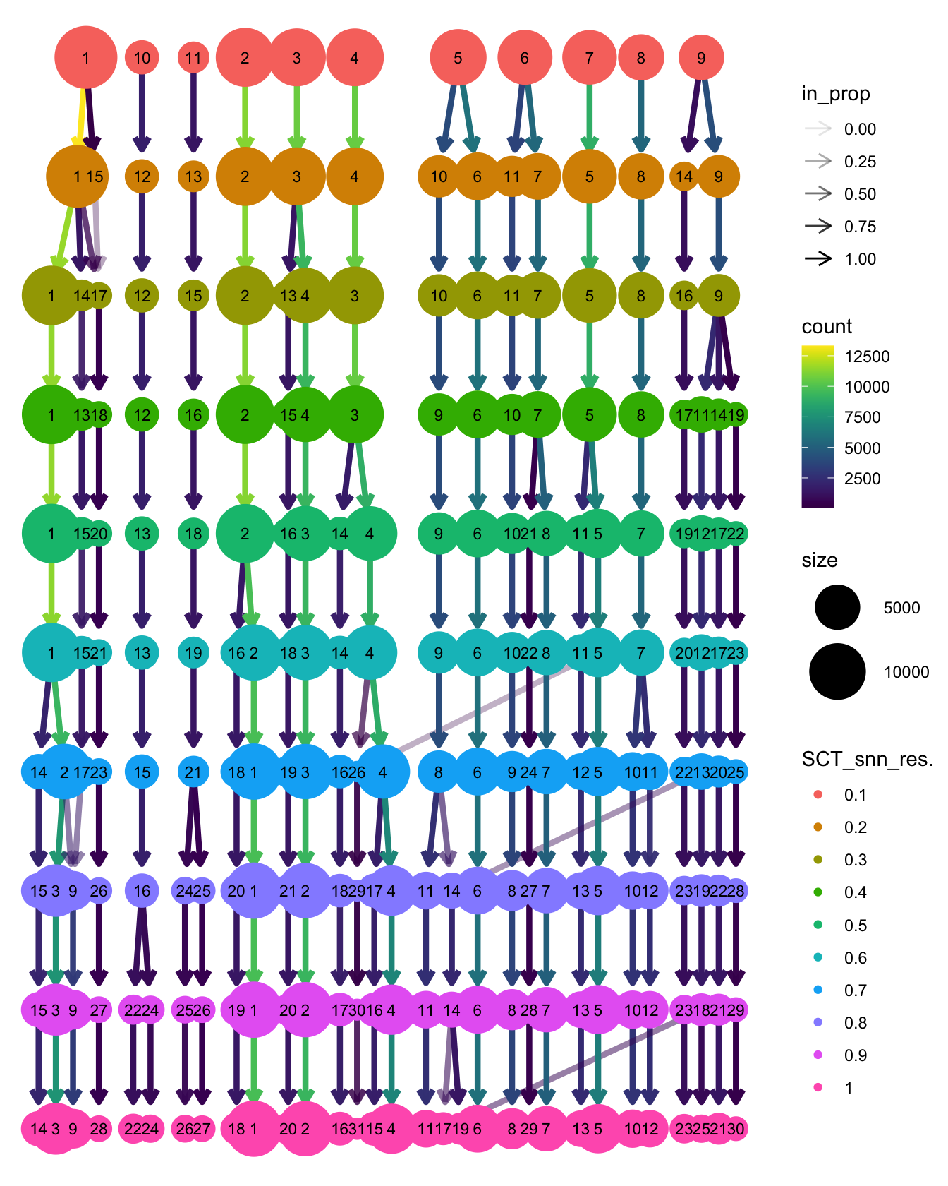
Resolution 0.1 cleanly separates each patient’s blast population into
its own cluster. The normal bone marrow clusters (8, 10, 11) will be
sub-clustered by re-embedding just those cells on their own UMAP (see
below). For the initial visualisations, cluster_final is
set to the global res 0.1 labels.
seu$cluster_final <- as.character(seu$SCT_snn_res.0.1)
table(seu$cluster_final)
    1    10    11     2     3     4     5     6     7     8     9
13483  1822  1318 11241 10673 10590  9939  9119  8950  5344  5055
Examine UMAPs
Visualise the joint UMAP coloured by cluster, sample, cell type, batch, cell cycle phase, and fusion detection.
grp <- "cluster_final"

DimPlot(seu, reduction = "umap", label = TRUE, repel = TRUE,
        label.size = 2.5, group.by = grp) +
  theme(legend.position = "bottom") -> p1

DimPlot(seu, reduction = "umap", label = FALSE, repel = TRUE,
        group.by = "patient_timepoint") +
  paletteer::scale_color_paletteer_d("pals::glasbey") +
  guides(colour = guide_legend(ncol = 2, override.aes = list(size = 3))) +
  theme(legend.position = "bottom") -> p2

p1 | p2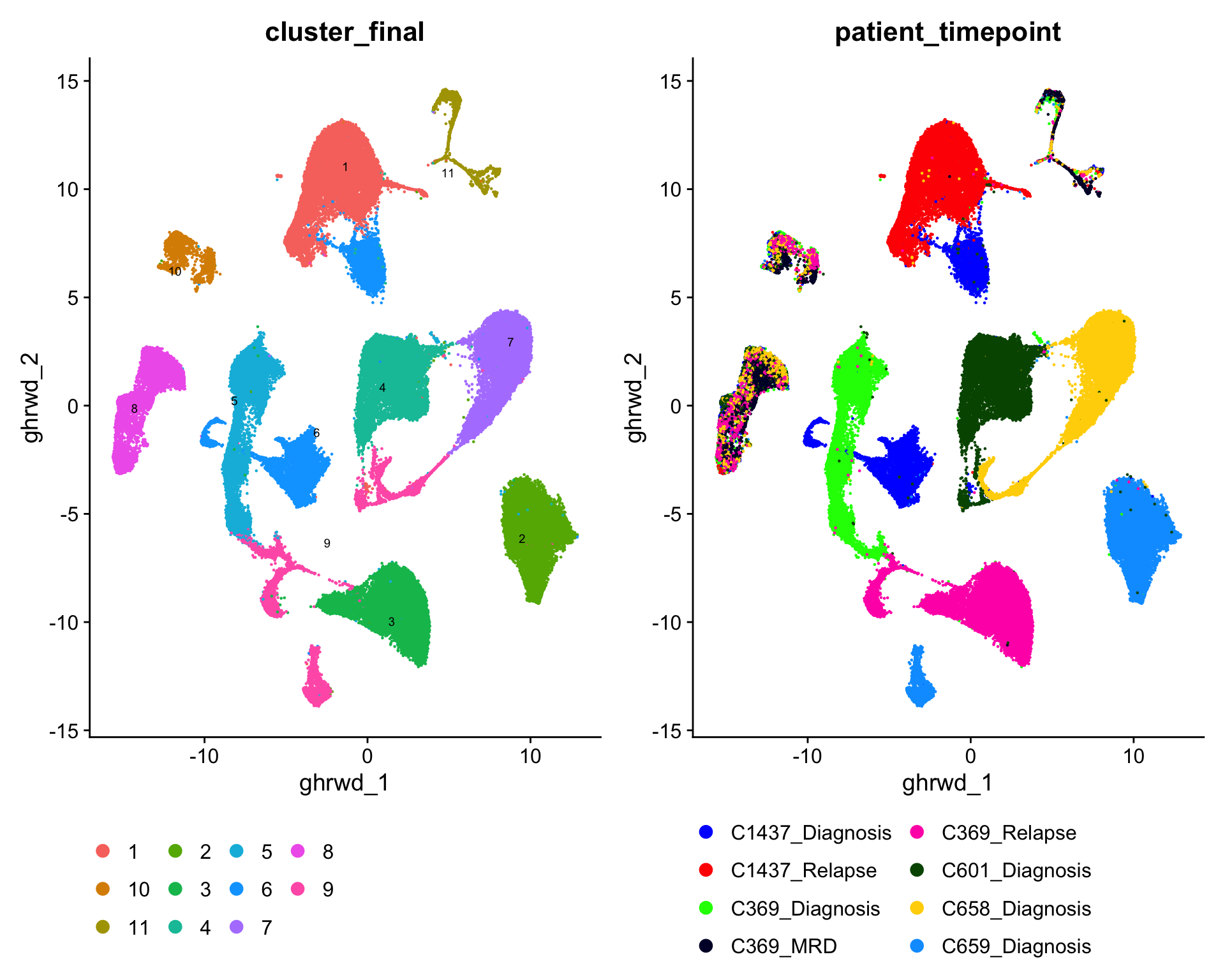
DimPlot(seu, reduction = "umap", label = TRUE, repel = TRUE,
        label.size = 2.5, group.by = "predicted_CellType_Broad") +
  paletteer::scale_color_paletteer_d("pals::glasbey") +
  NoLegend() -> p3

p3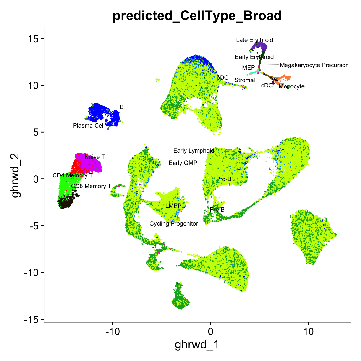
DimPlot(seu, reduction = "umap", label = FALSE,
        group.by = grp,
        cells.highlight = which(seu$patient_fusion != "not-detected"),
        sizes.highlight = 0.1) +
  ggtitle("Fusion detection") +
  NoLegend() -> p5

DimPlot(seu, reduction = "umap", label = TRUE, repel = TRUE,
        label.size = 2.5, group.by = "Phase") +
  scale_color_manual(values = c("G1"  = "#E69F00",
                                "G2M" = "#56B4E9",
                                "S"   = "#009E73")) +
  theme(legend.position = "bottom") -> p6

p5 | p6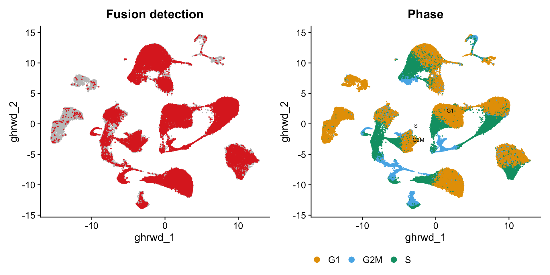
Normal BM re-embedding
The global UMAP is dominated by blast variation — patient-specific blast islands occupy most of the embedding space, compressing normal BM cells into a small region where lineage structure is not visible. The T/NK compartment (global cluster 8) and the B/myeloid/erythroid compartment (global clusters 10, 11) are driven by fundamentally different variable genes, so they are re-embedded separately. This allows each compartment’s own biology to drive the HVG selection, PCA, and UMAP layout.
T/NK compartment (cluster 8)
out_tnk <- here("data", "RDS", "exp2_tnk_bm.seu.rds")

if (!file.exists(out_tnk)) {
  seu_tnk <- subset(seu, SCT_snn_res.0.1 == "8")

  DefaultAssay(seu_tnk) <- "RNA"
  seu_tnk[["RNA"]] <- JoinLayers(seu_tnk[["RNA"]])

  seu_tnk <- SCTransform(seu_tnk, verbose = FALSE,
                         return.only.var.genes = FALSE)

  DefaultAssay(seu_tnk) <- "SCT"
  seu_tnk <- RunPCA(seu_tnk, verbose = FALSE, npcs = 30, assay = "SCT")
  seu_tnk <- FindNeighbors(seu_tnk, reduction = "pca", dims = 1:30)
  seu_tnk <- FindClusters(seu_tnk, resolution = seq(0.1, 1, by = 0.1),
                          algorithm = "Leiden")
  seu_tnk <- RunUMAP(seu_tnk, dims = 1:30, reduction = "pca")

  saveRDS(seu_tnk, file = out_tnk)
  fs::file_chmod(out_tnk, "664")
  try(fs::file_chown(out_tnk, group_id = "oshlack_lab"), silent = TRUE)

} else {
  seu_tnk <- readRDS(out_tnk)
}
clustree(seu_tnk, prefix = "SCT_snn_res.")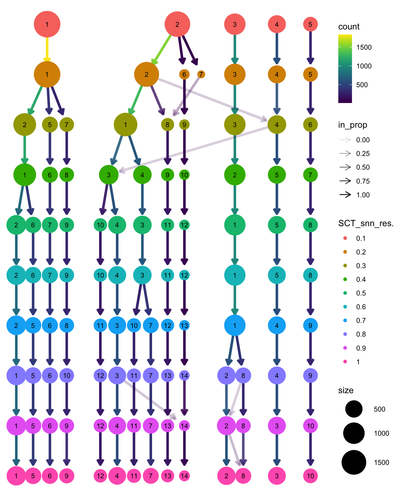
tnk_res <- "SCT_snn_res.0.3"

DimPlot(seu_tnk, reduction = "umap", label = TRUE, repel = TRUE,
        label.size = 3, group.by = tnk_res) +
  NoLegend() -> p1

DimPlot(seu_tnk, reduction = "umap", label = TRUE, repel = TRUE,
        label.size = 3, group.by = "predicted_CellType_Broad") +
  paletteer::scale_color_paletteer_d("pals::glasbey") +
  NoLegend() -> p2

p1 | p2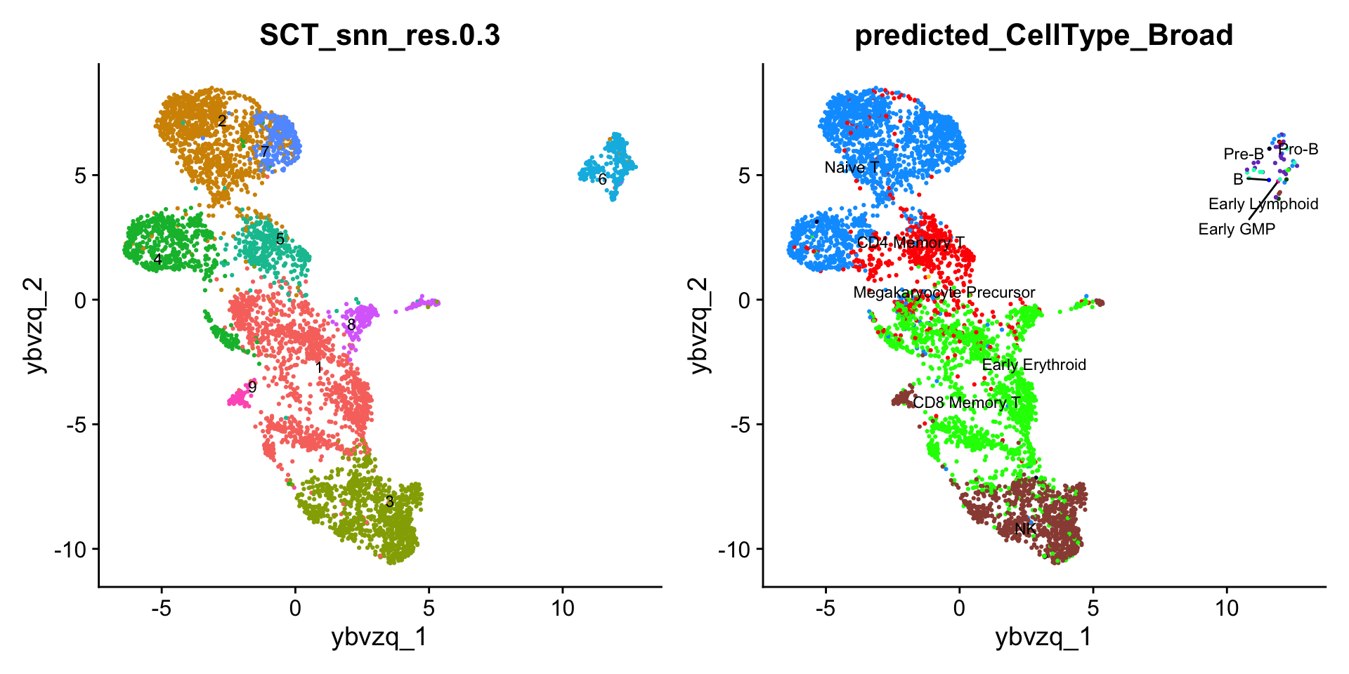
B/myeloid/erythroid compartment (clusters 10, 11)
out_nontnk <- here("data", "RDS", "exp2_nontnk_bm.seu.rds")

if (!file.exists(out_nontnk)) {
  seu_nontnk <- subset(seu, SCT_snn_res.0.1 %in% c("10", "11"))

  DefaultAssay(seu_nontnk) <- "RNA"
  seu_nontnk[["RNA"]] <- JoinLayers(seu_nontnk[["RNA"]])

  seu_nontnk <- SCTransform(seu_nontnk, verbose = FALSE,
                            return.only.var.genes = FALSE)

  DefaultAssay(seu_nontnk) <- "SCT"
  seu_nontnk <- RunPCA(seu_nontnk, verbose = FALSE, npcs = 30, assay = "SCT")
  seu_nontnk <- FindNeighbors(seu_nontnk, reduction = "pca", dims = 1:30)
  seu_nontnk <- FindClusters(seu_nontnk, resolution = seq(0.1, 1, by = 0.1),
                             algorithm = "Leiden")
  seu_nontnk <- RunUMAP(seu_nontnk, dims = 1:30, reduction = "pca")

  saveRDS(seu_nontnk, file = out_nontnk)
  fs::file_chmod(out_nontnk, "664")
  try(fs::file_chown(out_nontnk, group_id = "oshlack_lab"), silent = TRUE)

} else {
  seu_nontnk <- readRDS(out_nontnk)
}
clustree(seu_nontnk, prefix = "SCT_snn_res.")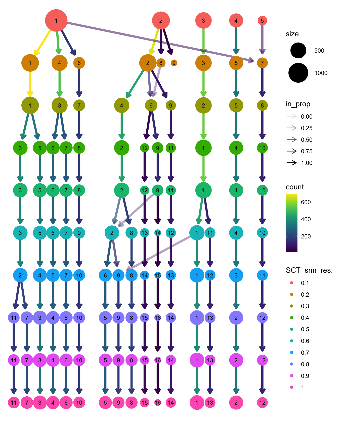
nontnk_res <- "SCT_snn_res.0.3"

DimPlot(seu_nontnk, reduction = "umap", label = TRUE, repel = TRUE,
        label.size = 3, group.by = nontnk_res) +
  NoLegend() -> p1

DimPlot(seu_nontnk, reduction = "umap", label = TRUE, repel = TRUE,
        label.size = 3, group.by = "predicted_CellType_Broad") +
  paletteer::scale_color_paletteer_d("pals::glasbey") +
  NoLegend() -> p2

p1 | p2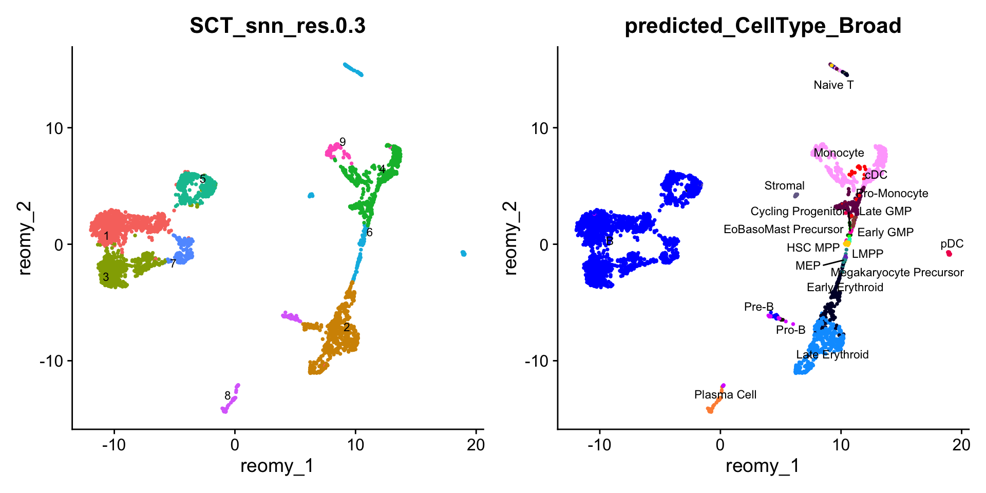
Cluster quality checks
Three sub-embedding clusters are inspected before label transfer:
tnk_6 (an isolated population in the T/NK sub-embedding
annotated as B-precursors with high mapping error and elevated fusion
detection), bm_6 (the heterogeneous multipotent progenitor
cluster in the B/myeloid/erythroid sub-embedding whose majority vote
ties between HSC MPP and Early Erythroid), and bm_8 (a
Plasma Cell cluster with minor B-precursor admixture). Each is flagged
in the main seu object and examined for QC metrics, doublet
and mapping error status, patient composition, fine cell type identity,
and fusion detection rate.
tnk_cluster6 <- rownames(seu_tnk@meta.data[seu_tnk$SCT_snn_res.0.3 == "6", ])
bm_cluster6  <- rownames(seu_nontnk@meta.data[seu_nontnk$SCT_snn_res.0.3 == "6", ])
bm_cluster8  <- rownames(seu_nontnk@meta.data[seu_nontnk$SCT_snn_res.0.3 == "8", ])

seu$cluster_interest <- case_when(
  colnames(seu) %in% tnk_cluster6 ~ "tnk_6",
  colnames(seu) %in% bm_cluster6  ~ "bm_6",
  colnames(seu) %in% bm_cluster8  ~ "bm_8",
  TRUE ~ "other"
)

# Where do these clusters sit in the joint UMAP?
DimPlot(seu, group.by = "cluster_interest",
        cols = c("tnk_6" = "red", "bm_6" = "blue", "bm_8" = "green", "other" = "grey90")) +
  ggtitle("Clusters of interest in joint UMAP")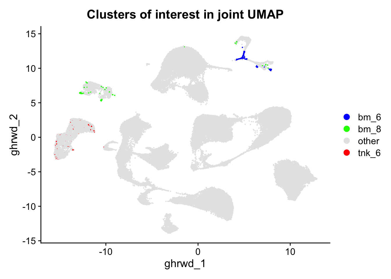
# QC metrics — are these low quality, doublets, or poor mapping?
seu@meta.data %>%
  filter(cluster_interest != "other") %>%
  pivot_longer(cols = c(nFeature_RNA, nCount_RNA, scDblFinder.score, mapping_error_score),
               names_to = "metric") %>%
  ggplot(aes(x = cluster_interest, y = value, fill = cluster_interest)) +
  geom_violin(draw_quantiles = 0.5) +
  facet_wrap(~metric, scales = "free_y") +
  theme_minimal() +
  theme(legend.position = "none")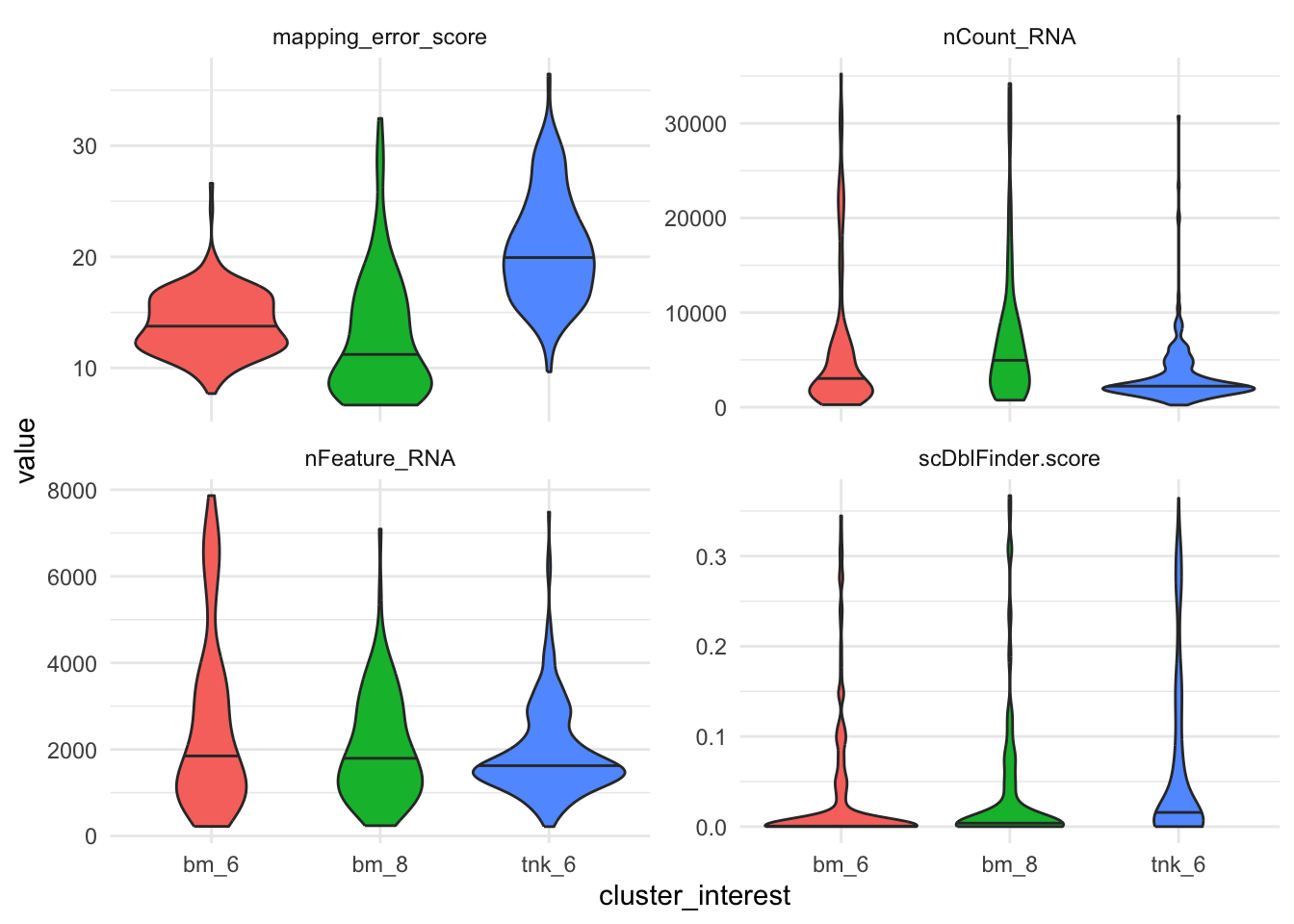
# Doublet + mapping QC pass/fail
seu@meta.data %>%
  filter(cluster_interest != "other") %>%
  group_by(cluster_interest, scDblFinder.class, mapping_error_QC) %>%
  tally()
# A tibble: 6 × 4
# Groups: cluster_interest, scDblFinder.class [3]
cluster_interest scDblFinder.class mapping_error_QC n
<chr> <fct> <chr> <int>
1 bm_6 singlet Fail 14
2 bm_6 singlet Pass 189
3 bm_8 singlet Fail 23
4 bm_8 singlet Pass 96
5 tnk_6 singlet Fail 239
6 tnk_6 singlet Pass 46# Patient composition — critical for tnk_6
seu@meta.data %>%
filter(cluster_interest != "other") %>%
dplyr::count(cluster_interest, patient_timepoint) %>%
arrange(cluster_interest, desc(n)) cluster_interest patient_timepoint n
1 bm_6 C369_MRD 73
2 bm_6 C1437_Relapse 39
3 bm_6 C658_Diagnosis 32
4 bm_6 C369_Diagnosis 27
5 bm_6 C369_Relapse 12
6 bm_6 C659_Diagnosis 10
7 bm_6 C1437_Diagnosis 8
8 bm_6 C601_Diagnosis 2
9 bm_8 C369_Diagnosis 34
10 bm_8 C1437_Relapse 22
11 bm_8 C658_Diagnosis 21
12 bm_8 C369_Relapse 17
13 bm_8 C601_Diagnosis 10
14 bm_8 C1437_Diagnosis 5
15 bm_8 C369_MRD 5
16 bm_8 C659_Diagnosis 5
17 tnk_6 C369_Diagnosis 126
18 tnk_6 C1437_Diagnosis 42
19 tnk_6 C1437_Relapse 33
20 tnk_6 C369_Relapse 29
21 tnk_6 C658_Diagnosis 26
22 tnk_6 C601_Diagnosis 15
23 tnk_6 C659_Diagnosis 14# Fine cell type breakdown
seu@meta.data %>%
filter(cluster_interest != "other") %>%
dplyr::count(cluster_interest, predicted_CellType) %>%
arrange(cluster_interest, desc(n)) cluster_interest predicted_CellType n
1 bm_6 pDC 19
2 bm_6 HSC 17
3 bm_6 BFU-E 16
4 bm_6 CFU-E 16
5 bm_6 Basophilic Erythroblast 15
6 bm_6 Stromal 15
7 bm_6 <NA> 14
8 bm_6 CD14 Mono 11
9 bm_6 Late ProMono 11
10 bm_6 Early GMP 9
11 bm_6 MPP-MyLy 9
12 bm_6 Orthochromatic Erythroblast 8
13 bm_6 EoBasoMast Precursor 6
14 bm_6 MPP-MkEry 6
15 bm_6 CD4 Naive 5
16 bm_6 LMPP 5
17 bm_6 MEP 4
18 bm_6 Megakaryocyte Precursor 4
19 bm_6 Cycling Progenitor 3
20 bm_6 GMP-Neut 3
21 bm_6 Early ProMono 1
22 bm_6 GMP-Mono 1
23 bm_6 Mature B 1
24 bm_6 Megakaryocyte 1
25 bm_6 Pre-pDC 1
26 bm_6 Pre-pDC Cycling 1
27 bm_6 Pro-Erythroblast 1
28 bm_8 Plasma Cell 58
29 bm_8 <NA> 23
30 bm_8 Small Pre-B 12
31 bm_8 Pro-B VDJ 9
32 bm_8 Immature B 8
33 bm_8 Mature B 6
34 bm_8 Large Pre-B 3
35 tnk_6 <NA> 239
36 tnk_6 Pro-B VDJ 21
37 tnk_6 Large Pre-B 5
38 tnk_6 CD4 Naive 4
39 tnk_6 Small Pre-B 4
40 tnk_6 Basophilic Erythroblast 2
41 tnk_6 NK CD56high 2
42 tnk_6 CD4 Effector Memory 1
43 tnk_6 CD8 Effector Memory 2 1
44 tnk_6 CD8 Naive 1
45 tnk_6 CLP 1
46 tnk_6 Early GMP 1
47 tnk_6 MLP 1
48 tnk_6 Mature B 1
49 tnk_6 Pro-B Cycling 1# Fusion status
seu@meta.data %>%
filter(cluster_interest != "other") %>%
group_by(cluster_interest, fusion_detected) %>%
tally()# A tibble: 6 × 3
# Groups: cluster_interest [3]
cluster_interest fusion_detected n
<chr> <lgl> <int>
1 bm_6 FALSE 191
2 bm_6 TRUE 12
3 bm_8 FALSE 102
4 bm_8 TRUE 17
5 tnk_6 FALSE 225
6 tnk_6 TRUE 60tnk_6 has high mapping error (84% of cells fail
mapping_error_QC) and elevated fusion detection (21%
fusion-positive) despite all cells being called singlets by scDblFinder.
The dot plot below tests whether these cells co-express T/NK and
blast/B-precursor markers — the hallmark of doublets or heavily
ambient-contaminated cells — or whether they are genuinely B-precursor
in identity.
markers_tnk6 <- c(
  # T/NK markers
  "CD3E", "CD8A", "CD4", "NKG7", "GNLY",
  # B-precursor / blast markers
  "CD19", "CD79A", "DNTT", "MME", "VPREB1"
)

DotPlot(seu_tnk,
        features = markers_tnk6,
        group.by = "SCT_snn_res.0.3") +
  geom_vline(xintercept = 5.5, linetype = "dashed", colour = "grey50") +
  scale_colour_distiller(palette = "RdYlBu") +
  coord_flip() +
  ggtitle("T/NK vs blast markers across T/NK sub-clusters")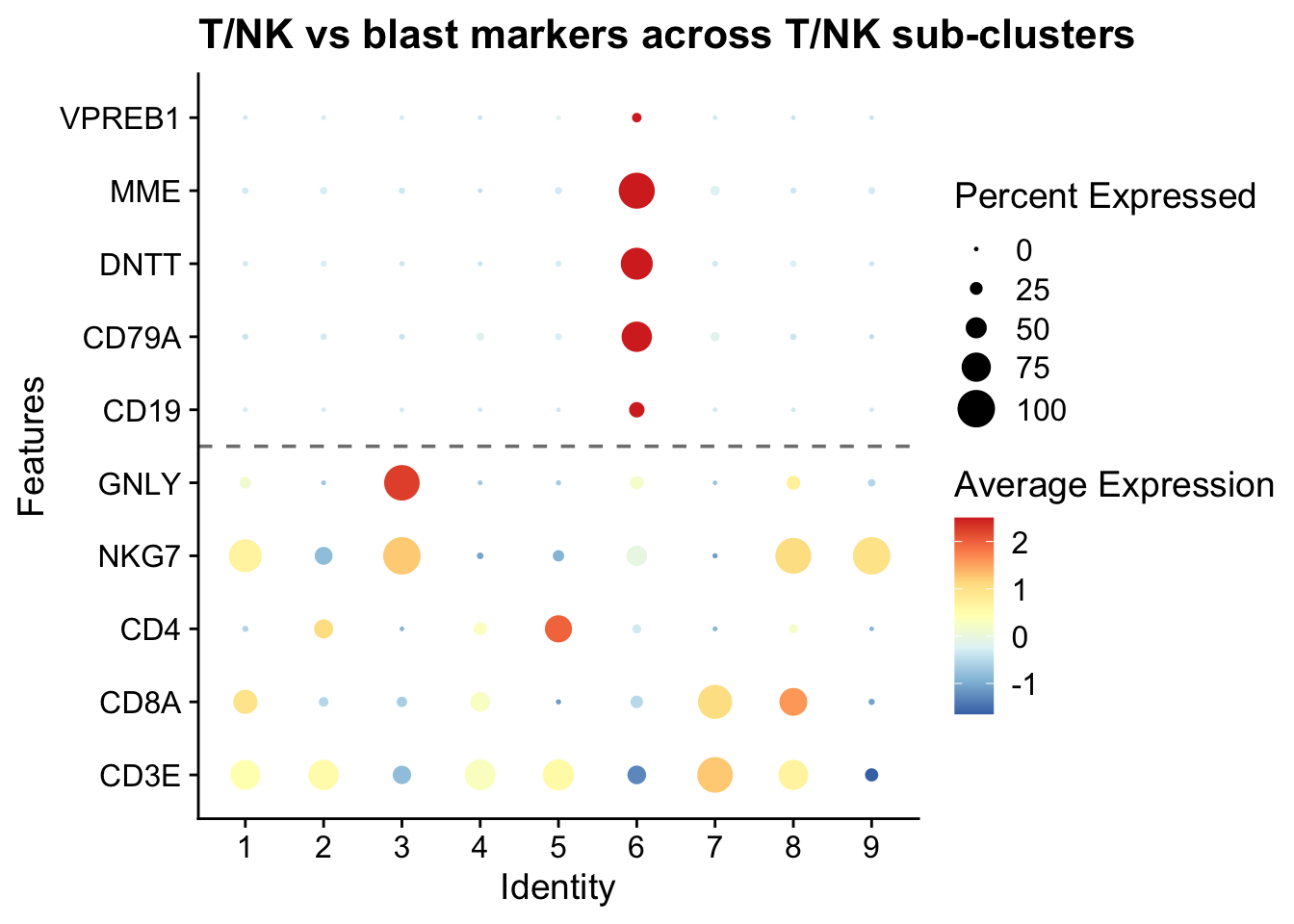
Cluster 6 expresses canonical B-precursor markers (MME, DNTT, CD79A) strongly with negligible T/NK signal — confirming these are genuine B-precursor cells (likely blast B-precursors that co-embedded with T/NK at global resolution 0.1) rather than doublets or ambient artefacts. No filtering is required; they receive a B-precursor Broad label via majority vote of mapping-passing cells.
bm_6 majority-votes to a tie between HSC MPP and Early
Erythroid due to its heterogeneous progenitor composition (HSC, MEP,
LMPP, pDC, Megakaryocyte Precursor and others). bm_8
contains Plasma Cells alongside a minor B-precursor population. The dot
plot below confirms cluster identities using terminal lineage
markers.
markers_bm <- c(
  # HSC / progenitor
  "CD34", "AVP",
  # Erythroid
  "HBB", "GYPA",
  # Myeloid
  "CD14", "S100A8",
  # pDC
  "IL3RA",
  # B-precursor
  "DNTT", "MME", "CD19",
  # B cell
  "MS4A1", "CD79A",
  # Plasma cell
  "MZB1", "IGHG1"
)

DotPlot(seu_nontnk,
        features = markers_bm,
        group.by = "SCT_snn_res.0.3") +
  scale_colour_distiller(palette = "RdYlBu") +
  coord_flip() +
  ggtitle("Lineage markers across non-T/NK sub-clusters")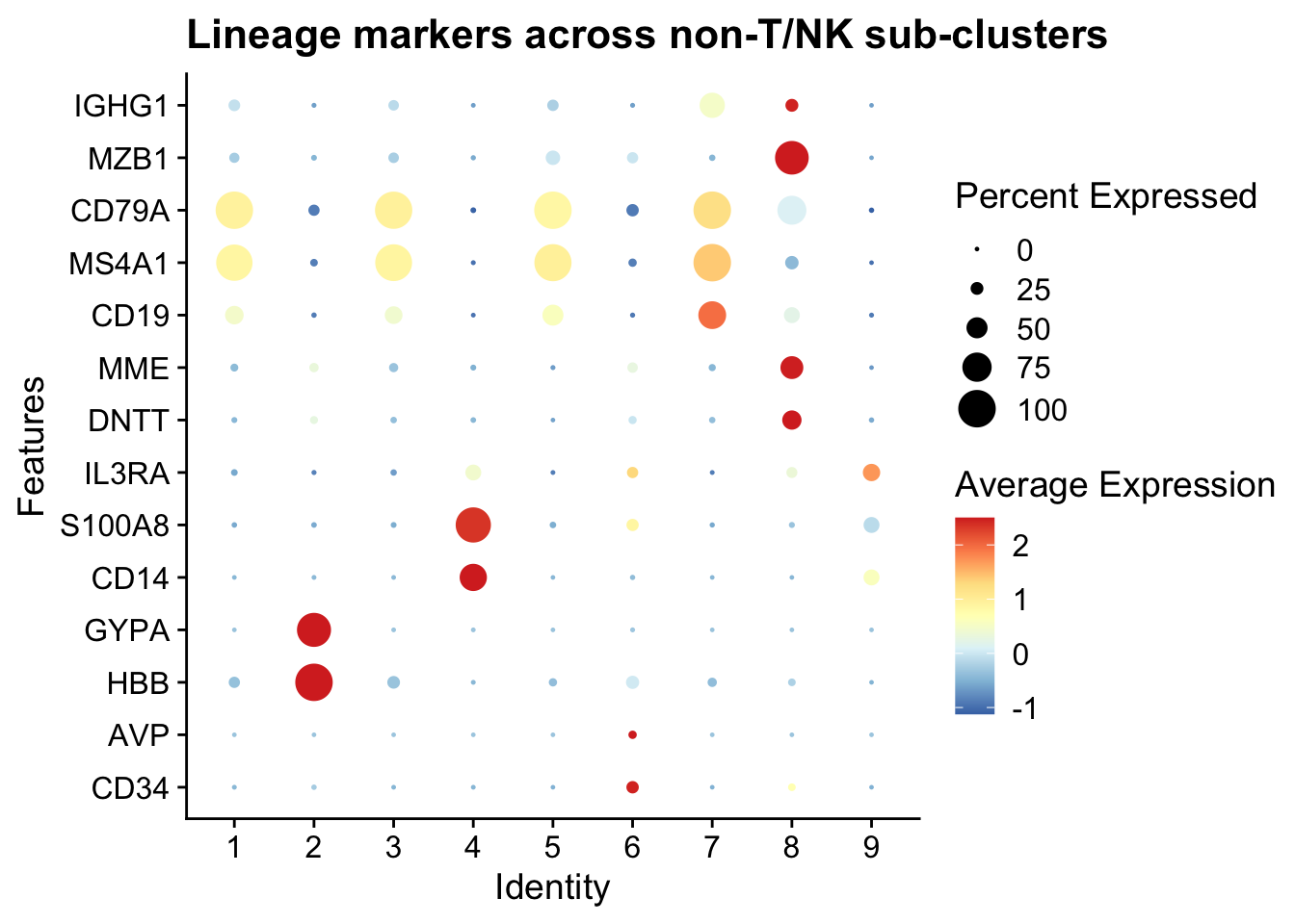
bm_6 is negative for all terminal lineage markers with
only faint CD34 and IL3RA signal, consistent with multipotent
progenitors; it is overridden to "HSC MPP" in the
annotation step. bm_8 shows strong MZB1 and IGHG1
confirming Plasma Cell identity, with a minor MME/DNTT signal from the
co-embedded B-precursor cells. FindSubCluster is used to
separate these two populations before label transfer.
Sub-cluster bm_8
bm_8 contains two biologically distinct populations:
Plasma Cells (n = 58) and B-precursor cells (Pre-B/Pro-B, n = 36).
FindSubCluster is run on cluster 8 of the non-T/NK
sub-embedding to resolve these into bm_8_1 (Plasma Cell)
and bm_8_2 (Pre-B) before transferring labels to the main
object. Sub-clustering was also attempted on bm_2 (Late/Early Erythroid)
but the erythroid maturation trajectory is continuous and no resolution
cleanly separated the two populations; bm_2 retains its “Late Erythroid”
majority-vote label.
Idents(seu_nontnk) <- "SCT_snn_res.0.3"

seu_nontnk <- FindSubCluster(
  seu_nontnk,
  cluster         = "8",
  graph.name      = "SCT_snn",
  subcluster.name = "sub.cluster",
  resolution      = 0.3,
  algorithm       = 4
)

# Verify the split: 8_1 = Plasma Cell, 8_2 = Pre-B/Pro-B
table(
  seu_nontnk$sub.cluster[seu_nontnk$SCT_snn_res.0.3 == "8"],
  seu_nontnk$predicted_CellType_Broad[seu_nontnk$SCT_snn_res.0.3 == "8"]
)
       B Plasma Cell Pre-B Pro-B
  8_1  2          58     0     0
  8_2 12           0    15     9
# Build cluster_for_transfer: use sub.cluster for bm_8 cells, original res 0.3 elsewhere
seu_nontnk$cluster_for_transfer <- ifelse(
seu_nontnk$SCT_snn_res.0.3 == "8",
seu_nontnk$sub.cluster,
as.character(seu_nontnk$SCT_snn_res.0.3)
)Transfer normal BM labels to main object
Once resolutions are chosen for both sub-embeddings, cluster labels
are transferred back to the main seu object. Blast clusters
keep their global res 0.1 integer labels; T/NK cells get labels prefixed
with tnk_ and B/myeloid/erythroid cells with
bm_. For the non-T/NK compartment,
cluster_for_transfer is used instead of the raw resolution
column so that bm_8 is transferred as two sub-clusters
(bm_8_1 and bm_8_2) rather than a single
bm_8 label.
tnk_res    <- "SCT_snn_res.0.3"
nontnk_res <- "SCT_snn_res.0.3"

# Start from global res 0.1
seu$cluster_final <- as.character(seu$SCT_snn_res.0.1)

# T/NK labels
tnk_meta   <- seu_tnk@meta.data[, tnk_res, drop = FALSE]
tnk_labels <- paste0("tnk_", tnk_meta[[tnk_res]])
names(tnk_labels) <- rownames(tnk_meta)
seu$cluster_final[names(tnk_labels)] <- tnk_labels

# B/myeloid/erythroid labels — use cluster_for_transfer so bm_8 is split into
# bm_8_1 (Plasma Cell) and bm_8_2 (Pre-B) via FindSubCluster above
nontnk_meta   <- seu_nontnk@meta.data[, "cluster_for_transfer", drop = FALSE]
nontnk_labels <- paste0("bm_", nontnk_meta[["cluster_for_transfer"]])
names(nontnk_labels) <- rownames(nontnk_meta)
seu$cluster_final[names(nontnk_labels)] <- nontnk_labels

table(seu$cluster_final)
     1      2      3      4      5      6      7      9   bm_1   bm_2   bm_3
 13483  11241  10673  10590   9939   9119   8950   5055    693    560    525
  bm_4   bm_5   bm_6   bm_7 bm_8_1 bm_8_2   bm_9  tnk_1  tnk_2  tnk_3  tnk_4
   445    333    203    169     62     57     93   1316   1188    989    650
 tnk_5  tnk_6  tnk_7  tnk_8  tnk_9
   372    285    279    185     80
PC loading analysis: why do tnk_6 blast B-precursors co-embed with T/NK?
# Key genes to track
genes_tnk    <- c("CD3D", "CD3E", "CD3G", "CD3Z", "NKG7", "GNLY", "GZMB", "GZMK")
genes_bpre   <- c("DNTT", "MME", "CD79A", "CD79B", "VPREB1", "VPREB3", "IGLL1")
genes_blast  <- c("ETV6", "RUNX1", "CDK6", "EBF1")
genes_of_int <- c(genes_tnk, genes_bpre, genes_blast)

hvgs <- VariableFeatures(seu)
cat("=== HVG membership (top 3000) ===\n")
=== HVG membership (top 3000) ===for (g in genes_of_int) {
r <- match(g, hvgs)
cat(sprintf(" %-10s in HVGs: %-5s rank: %s\n", g,
!is.na(r), ifelse(is.na(r), "–", r)))
} CD3D in HVGs: TRUE rank: 161
CD3E in HVGs: TRUE rank: 121
CD3G in HVGs: TRUE rank: 244
CD3Z in HVGs: FALSE rank: –
NKG7 in HVGs: TRUE rank: 16
GNLY in HVGs: TRUE rank: 14
GZMB in HVGs: TRUE rank: 185
GZMK in HVGs: TRUE rank: 59
DNTT in HVGs: TRUE rank: 420
MME in HVGs: TRUE rank: 255
CD79A in HVGs: TRUE rank: 301
CD79B in HVGs: TRUE rank: 501
VPREB1 in HVGs: TRUE rank: 507
VPREB3 in HVGs: TRUE rank: 991
IGLL1 in HVGs: TRUE rank: 1245
ETV6 in HVGs: TRUE rank: 1375
RUNX1 in HVGs: TRUE rank: 1222
CDK6 in HVGs: TRUE rank: 1639
EBF1 in HVGs: TRUE rank: 578# Mean PC embedding per global Leiden cluster
pca_embed <- Embeddings(seu, "pca")
loadings <- Loadings(seu, reduction = "pca")
pc_means <- sapply(sort(unique(seu$SCT_snn_res.0.1)), function(cl) {
colMeans(pca_embed[seu$SCT_snn_res.0.1 == cl, , drop = FALSE])
})
colnames(pc_means) <- sort(unique(seu$SCT_snn_res.0.1))
# Blast clusters vs T/NK cluster (8) — which PCs drive the split?
blast_cls <- as.character(c(1:7, 9))
pc_tnk <- pc_means[, "8"]
pc_blast <- rowMeans(pc_means[, blast_cls, drop = FALSE])
pc_diff <- pc_tnk - pc_blast
cat("\n=== PCs most separating cluster 8 (T/NK) from blast clusters ===\n")
=== PCs most separating cluster 8 (T/NK) from blast clusters ===print(sort(abs(pc_diff), decreasing = TRUE)[1:10]) PC_1 PC_3 PC_6 PC_2 PC_7 PC_13 PC_8
49.8617904 29.2924337 11.8246146 4.8577815 3.2992646 3.1085309 1.2726765
PC_5 PC_14 PC_9
0.9376841 0.8288629 0.8243907 top_pcs <- names(sort(abs(pc_diff), decreasing = TRUE)[1:5])
for (pc in top_pcs) {
cat(sprintf("\n--- %s (T/NK vs blast difference: %.3f) ---\n",
pc, pc_diff[pc]))
cat("Top positive:\n")
print(sort(loadings[, pc], decreasing = TRUE)[1:10])
cat("Top negative:\n")
print(sort(loadings[, pc], decreasing = FALSE)[1:10])
# Where do our genes of interest rank in this PC?
present <- genes_of_int[genes_of_int %in% rownames(loadings)]
gene_ranks <- sort(loadings[present, pc], decreasing = pc_diff[pc] > 0)
cat("Genes of interest in this PC:\n")
print(gene_ranks)
}
--- PC_1 (T/NK vs blast difference: -49.862) ---
Top positive:
       MME   HIST1H1B       RAG1       DNTT      UHRF1       CD24       H1F0
0.04187456 0.03502376 0.03254634 0.03048634 0.02787326 0.02687334 0.02630574
      TYMS   HIST1H1C      TCL1A
0.02541245 0.02464220 0.02430665
Top negative:
      SRGN       NKG7       CCL5       IL32       PRF1       GNLY        LYZ
-0.2305065 -0.2176174 -0.1661240 -0.1405037 -0.1346970 -0.1337849 -0.1253554
     TRBC2      ANXA1       GZMA
-0.1241567 -0.1229430 -0.1222334
Genes of interest in this PC:
        NKG7         GNLY         CD3E         GZMK         CD3D         GZMB
-0.217617423 -0.133784854 -0.069010014 -0.056472269 -0.055906124 -0.047235748
        CD3G       VPREB1        IGLL1         CDK6         ETV6       VPREB3
-0.045761185  0.009052210  0.009615097  0.013268145  0.013523681  0.013717338
       RUNX1        CD79B         EBF1        CD79A         DNTT          MME
 0.014371774  0.018147498  0.019048943  0.021033015  0.030486337  0.041874559

--- PC_3 (T/NK vs blast difference: 29.292) ---
Top positive:
      NKG7       CCL5       IL32       PRF1       GNLY      TRBC2       GZMA
0.20254177 0.16271614 0.13537349 0.13193725 0.13014358 0.12158662 0.12009535
      CST7      IL2RB      KLRK1
0.11523861 0.10468763 0.09867151
Top negative:
       LYZ     S100A9     S100A8       VCAN     MS4A6A      MPEG1      THBS1
-0.2144177 -0.2062601 -0.1947294 -0.1570505 -0.1360524 -0.1202774 -0.1147262
      MNDA      PLBD1       FGL2
-0.1143718 -0.1073091 -0.1037400
Genes of interest in this PC:
        NKG7         GNLY         CD3E         GZMK         CD3D         CD3G
 0.202541769  0.130143577  0.067876089  0.056366190  0.055463703  0.045360083
        GZMB         CDK6        IGLL1       VPREB1       VPREB3         EBF1
 0.045256514 -0.001534019 -0.001657880 -0.002119472 -0.002640149 -0.003734637
       CD79B         ETV6        RUNX1         DNTT        CD79A          MME
-0.003948631 -0.004001654 -0.004170334 -0.007095921 -0.008025595 -0.009317838

--- PC_6 (T/NK vs blast difference: 11.825) ---
Top positive:
     TRBC2       TRAC       TCF7       IL32       CD3E      NELL2      TRBC1
0.26516915 0.24970321 0.19269648 0.12286868 0.11397591 0.11225859 0.10559972
      JUNB       CD3D        ITK
0.10321727 0.10079599 0.09748815
Top negative:
                      NKG7                       GNLY
                -0.2374920                 -0.2279253
                      IGKC DEPRECATED-ENSG00000211592
                -0.2250199                 -0.2015425
                      PRF1                       IGHM
                -0.1867651                 -0.1680850
                      IGHD                      KLRD1
                -0.1093154                 -0.1059505
                      CST7                      IL2RB
                -0.1027103                 -0.1025372
Genes of interest in this PC:
        CD3E         CD3D         CD3G         GZMK       VPREB1         CDK6
 0.113975906  0.100795988  0.079277394  0.045601099  0.001542904 -0.001751254
       IGLL1        RUNX1         ETV6       VPREB3         EBF1         DNTT
-0.001863125 -0.003568096 -0.005679698 -0.005699026 -0.007433872 -0.012232884
       CD79A        CD79B          MME         GZMB         GNLY         NKG7
-0.016467346 -0.021999283 -0.023643982 -0.079721388 -0.227925347 -0.237492011

--- PC_2 (T/NK vs blast difference: 4.858) ---
Top positive:
      NKG7       CCL5      TRBC2       IL32       PRF1       GNLY       GZMA
0.02831045 0.02161364 0.01885946 0.01853944 0.01739729 0.01703565 0.01600930
      CST7       IGHM       SRGN
0.01555792 0.01514099 0.01512311
Top negative:
DEPRECATED-ENSG00000244734                        HBB
                -0.2478838                 -0.2466206
                      HBA1                       HBA2
                -0.2438223                 -0.2420191
                       HBD                     SLC4A1
                -0.2235514                 -0.2190469
                       CA1                       AHSP
                -0.2134493                 -0.2021018
                       HBM                        CA2
                -0.1978196                 -0.1778334
Genes of interest in this PC:
       NKG7        GNLY         MME        CD3E        CD3D        GZMK
0.028310453 0.017035654 0.011291738 0.009559918 0.007814005 0.007598786
       DNTT       CD79B       RUNX1        CD3G        ETV6        GZMB
0.007320150 0.006972748 0.006566569 0.006355359 0.006354392 0.006182283
      CD79A        EBF1        CDK6      VPREB1      VPREB3       IGLL1
0.006047802 0.005898528 0.004132417 0.003570515 0.003062283 0.001346729

--- PC_7 (T/NK vs blast difference: -3.299) ---
Top positive:
      EGR1     JCHAIN        GSN     ADGRE5     ADGRG1       IER2      PLVAP
0.23394541 0.22368113 0.10060789 0.09834878 0.09825910 0.08407199 0.07873694
     HSPB1       PIM1      LAMA3
0.07549270 0.07455374 0.07366084
Top negative:
   HIST1H1B       CXCR4    HIST1H1C        IGHM       TRBC2        TRAC
-0.14760724 -0.11244941 -0.11032585 -0.10372139 -0.08310117 -0.07579977
       RAG1         JUN         MME        IGKC
-0.07210027 -0.07206175 -0.07050862 -0.06541036
Genes of interest in this PC:
         MME         CD3E         CD3D         GZMK         CD3G         DNTT
-0.070508622 -0.040093124 -0.035503869 -0.030317547 -0.027911212 -0.026712815
       CD79B         ETV6        RUNX1       VPREB3        IGLL1         EBF1
-0.010850048 -0.009989287 -0.002515208 -0.001647051 -0.000418305  0.001732843
        CDK6         GZMB         GNLY       VPREB1        CD79A         NKG7
 0.004490705  0.011610145  0.029836532  0.038878550  0.045879342  0.054158137
What this tells you:
- HVG membership — whether DNTT, MME, CD79A etc. are even in the 3000 HVGs at all, and if so, their rank
- PC difference — which PCs have the largest mean-embedding gap between cluster 8 (T/NK) and the blast clusters
- Gene loadings for those PCs — whether the top-loaded genes are T/NK markers, B-precursor markers, or something else
- Genes of interest ranks — where the blast/B-precursor/T/NK genes land within the most discriminating PCs
If the hypothesis is right, you’d expect: B-precursor genes either absent from HVGs or ranked low in the PCs that most separate cluster 8 from blasts, while T/NK genes dominate the positive loadings of those PCs.
Annotate clusters
Clusters are annotated using majority vote of the BoneMarrowMap
predicted_CellType_Broad label. For T/NK and normal BM
clusters, only cells passing mapping_error_QC are used for
voting. For blast clusters (integer labels), each cell is labelled
directly from its own patient_timepoint rather than by
cluster majority vote — this correctly handles cross-assigned cells and
mixed clusters (e.g. cluster 9, which contains blasts from both C658 and
C659 due to their shared ETV6::RUNX1-v2 breakpoint).
# Blast clusters = all cluster_final values that are NOT prefixed with tnk_ or bm_
# (determined dynamically after BM label transfer — robust across re-clusterings)
blast_clusters <- grep("^(tnk_|bm_)", unique(seu$cluster_final), value = TRUE, invert = TRUE)

# tnk_6 contains B-precursor blast cells that co-embedded with T/NK at global
# res 0.1 due to asymmetric PC loadings: T/NK marker genes rank 14–244 in the
# HVGs and load 5–8x more strongly on PC_1/PC_3 than B-precursor genes (rank
# 255–1245). These cells have 84% BoneMarrowMap mapping failure and 21% fusion
# detection — identical biology to the integer blast clusters. Add to
# blast_clusters so they receive per-patient labels rather than majority-vote BM labels.
if ("tnk_6" %in% seu$cluster_final) {
  blast_clusters <- union(blast_clusters, "tnk_6")
}

# bm_8_2 also contains blast B-precursor cells despite landing in the non-T/NK
# sub-embedding. Patient composition is enriched for high-blast-burden diagnosis
# and relapse samples (C658_Dx: 16, C369_Rel: 15, C369_Dx: 10, C601_Dx: 6)
# with zero contribution from C369_MRD — the opposite of what genuine residual
# normal Pre-B cells would show (C369_MRD has the lowest blast burden and most
# intact normal BM of any sample). Treated as blasts for the same reason as tnk_6.
if ("bm_8_2" %in% seu$cluster_final) {
  blast_clusters <- union(blast_clusters, "bm_8_2")
}

cat("Blast clusters identified:", paste(sort(blast_clusters), collapse = ", "), "\n")
Blast clusters identified: 1, 2, 3, 4, 5, 6, 7, 9, bm_8_2, tnk_6 # Majority BoneMarrowMap label for T/NK and normal BM clusters
bm_annotation <- seu@meta.data %>%
filter(!cluster_final %in% blast_clusters,
mapping_error_QC == "Pass") %>%
group_by(cluster_final) %>%
dplyr::count(predicted_CellType_Broad) %>%
slice_max(n, n = 1, with_ties = FALSE) %>%
dplyr::select(cluster_final, celltype_label = predicted_CellType_Broad)
# Apply BM cluster labels first
# as.character() prevents silent NA if celltype_label is a factor
seu$celltype_label <- as.character(bm_annotation$celltype_label)[
match(seu$cluster_final, bm_annotation$cluster_final)
]
# bm_6 is the mixed multipotent progenitor cluster (HSC, MEP, LMPP, pDC,
# Megakaryocyte Precursor and others) — majority vote ties between HSC MPP and
# Early Erythroid due to equal counts; override to HSC MPP as the most
# representative label. bm_2 is correctly Late Erythroid (Pro/Poly/Ortho-erythroblasts)
# and requires no override.
if ("bm_6" %in% seu$cluster_final) {
seu$celltype_label[seu$cluster_final == "bm_6"] <- "HSC MPP"
}
# For blast cells, label directly from each cell's own patient_timepoint
# (avoids majority-vote errors in mixed clusters, e.g. C658/C659 sharing a breakpoint)
blast_mask <- seu$cluster_final %in% blast_clusters
seu$celltype_label[blast_mask] <- seu$patient_timepoint[blast_mask] %>%
str_replace("_Diagnosis", "_Dx") %>%
str_replace("_Relapse", "_Rel") %>%
str_replace("_Remission", "_Rem") %>%
paste0("_blast")
# Guard: catch any cells that fell through annotation
na_count <- sum(is.na(seu$celltype_label))
if (na_count > 0) {
warning(na_count, " cells have NA celltype_label — filling from predicted_CellType_Broad")
seu$celltype_label[is.na(seu$celltype_label)] <- as.character(
seu$predicted_CellType_Broad[is.na(seu$celltype_label)]
)
}
# Verification: full annotation table + C369 MRD breakdown
cat("\n--- Cluster annotation table ---\n")
--- Cluster annotation table ---print(table(seu$cluster_final, seu$celltype_label))
             B C1437_Dx_blast C1437_Rel_blast C369_Dx_blast C369_MRD_blast
  1          0            122           13305            19              2
  2          0              7               0            11              0
  3          0              0               0             4              1
  4          0              2               1             4              0
  5          0             12               3          9854              0
  6          0           9015              38            18              0
  7          0              0               0             0              0
  9          0             16               3           668              0
  bm_1     693              0               0             0              0
  bm_2       0              0               0             0              0
  bm_3     525              0               0             0              0
  bm_4       0              0               0             0              0
  bm_5     333              0               0             0              0
  bm_6       0              0               0             0              0
  bm_7     169              0               0             0              0
  bm_8_1     0              0               0             0              0
  bm_8_2     0              3               5            10              0
  bm_9       0              0               0             0              0
  tnk_1      0              0               0             0              0
  tnk_2      0              0               0             0              0
  tnk_3      0              0               0             0              0
  tnk_4      0              0               0             0              0
  tnk_5      0              0               0             0              0
  tnk_6      0             42              33           126              0
  tnk_7      0              0               0             0              0
  tnk_8      0              0               0             0              0
  tnk_9      0              0               0             0              0

         C369_Rel_blast C601_Dx_blast C658_Dx_blast C659_Dx_blast CD4 Memory T
  1                   7            11            12             5            0
  2                   3            20             8         11192            0
  3               10662             3             2             1            0
  4                   7         10542            29             5            0
  5                  26            14            20            10            0
  6                   0            22             4            22            0
  7                   0            11          8939             0            0
  9                1070           570          1362          1366            0
  bm_1                0             0             0             0            0
  bm_2                0             0             0             0            0
  bm_3                0             0             0             0            0
  bm_4                0             0             0             0            0
  bm_5                0             0             0             0            0
  bm_6                0             0             0             0            0
  bm_7                0             0             0             0            0
  bm_8_1              0             0             0             0            0
  bm_8_2             15             6            16             2            0
  bm_9                0             0             0             0            0
  tnk_1               0             0             0             0            0
  tnk_2               0             0             0             0            0
  tnk_3               0             0             0             0            0
  tnk_4               0             0             0             0            0
  tnk_5               0             0             0             0          372
  tnk_6              29            15            26            14            0
  tnk_7               0             0             0             0            0
  tnk_8               0             0             0             0            0
  tnk_9               0             0             0             0            0

         CD8 Memory T HSC MPP Late Erythroid Monocyte Naive T    NK Plasma Cell
  1                 0       0              0        0       0     0           0
  2                 0       0              0        0       0     0           0
  3                 0       0              0        0       0     0           0
  4                 0       0              0        0       0     0           0
  5                 0       0              0        0       0     0           0
  6                 0       0              0        0       0     0           0
  7                 0       0              0        0       0     0           0
  9                 0       0              0        0       0     0           0
  bm_1              0       0              0        0       0     0           0
  bm_2              0       0            560        0       0     0           0
  bm_3              0       0              0        0       0     0           0
  bm_4              0       0              0      445       0     0           0
  bm_5              0       0              0        0       0     0           0
  bm_6              0     203              0        0       0     0           0
  bm_7              0       0              0        0       0     0           0
  bm_8_1            0       0              0        0       0     0          62
  bm_8_2            0       0              0        0       0     0           0
  bm_9              0       0              0       93       0     0           0
  tnk_1          1316       0              0        0       0     0           0
  tnk_2             0       0              0        0    1188     0           0
  tnk_3             0       0              0        0       0   989           0
  tnk_4             0       0              0        0     650     0           0
  tnk_5             0       0              0        0       0     0           0
  tnk_6             0       0              0        0       0     0           0
  tnk_7             0       0              0        0     279     0           0
  tnk_8           185       0              0        0       0     0           0
  tnk_9             0       0              0        0       0    80           0
cat("\n--- C369 MRD cell type composition ---\n")
--- C369 MRD cell type composition ---print(table(
seu$celltype_label[seu$patient_timepoint == "C369_MRD"],
useNA = "ifany"
))
             B C369_MRD_blast   CD4 Memory T   CD8 Memory T        HSC MPP
           398              3             15            150             73
Late Erythroid       Monocyte        Naive T             NK    Plasma Cell
           241            309            644            170              5
out <- here("data", "RDS", "exp2_joint_annotated.seu.rds")
if (!file.exists(out)) {
saveRDS(seu, file = out)
fs::file_chmod(out, "664")
try(fs::file_chown(out, group_id = "oshlack_lab"), silent = TRUE)
}# Run sort(unique(seu$celltype_label)) to verify all labels are covered
celltype_colors <- c(
# Blast clusters — one distinct hue per patient; lighter/darker for timepoints
"C601_Dx_blast" = "#4393C3", # blue
"C658_Dx_blast" = "#1A9850", # green
"C659_Dx_blast" = "#D73027", # red
"C1437_Dx_blast" = "#FDAE61", # light orange
"C1437_Rel_blast" = "#F46D43", # dark orange
"C369_MRD_blast" = "#DEC9E9", # pale lavender
"C369_Dx_blast" = "#9970AB", # medium purple
"C369_Rel_blast" = "#6A2E8A", # deep purple
# T/NK — all medium brightness, clearly different hues
"NK" = "#48DBFB", # bright cyan
"CD8 Memory T" = "#FF9FF3", # light magenta
"CD4 Memory T" = "#54A0FF", # cornflower blue
"Naive T" = "#A29BFE", # soft lavender
# B lineage
"Pre-B" = "#63CDDA", # light teal
"B" = "#26de81", # medium spring green
"Plasma Cell" = "#FAB1A0", # peach
# Myeloid
"Monocyte" = "#52B788", # mint green
# Erythroid / progenitor
"HSC MPP" = "#B39DDB", # soft lavender
"Late Erythroid" = "#D62246" # medium crimson
)
DimPlot(seu, reduction = "umap", label = TRUE, repel = TRUE,
label.size = 2.5, group.by = "celltype_label") +
scale_color_manual(values = celltype_colors) +
NoLegend() -> p1
DimPlot(seu, reduction = "umap", label = TRUE, repel = TRUE,
label.size = 2.5, group.by = "predicted_CellType_Broad") +
paletteer::scale_color_paletteer_d("pals::glasbey") +
NoLegend() -> p2
p1 | p2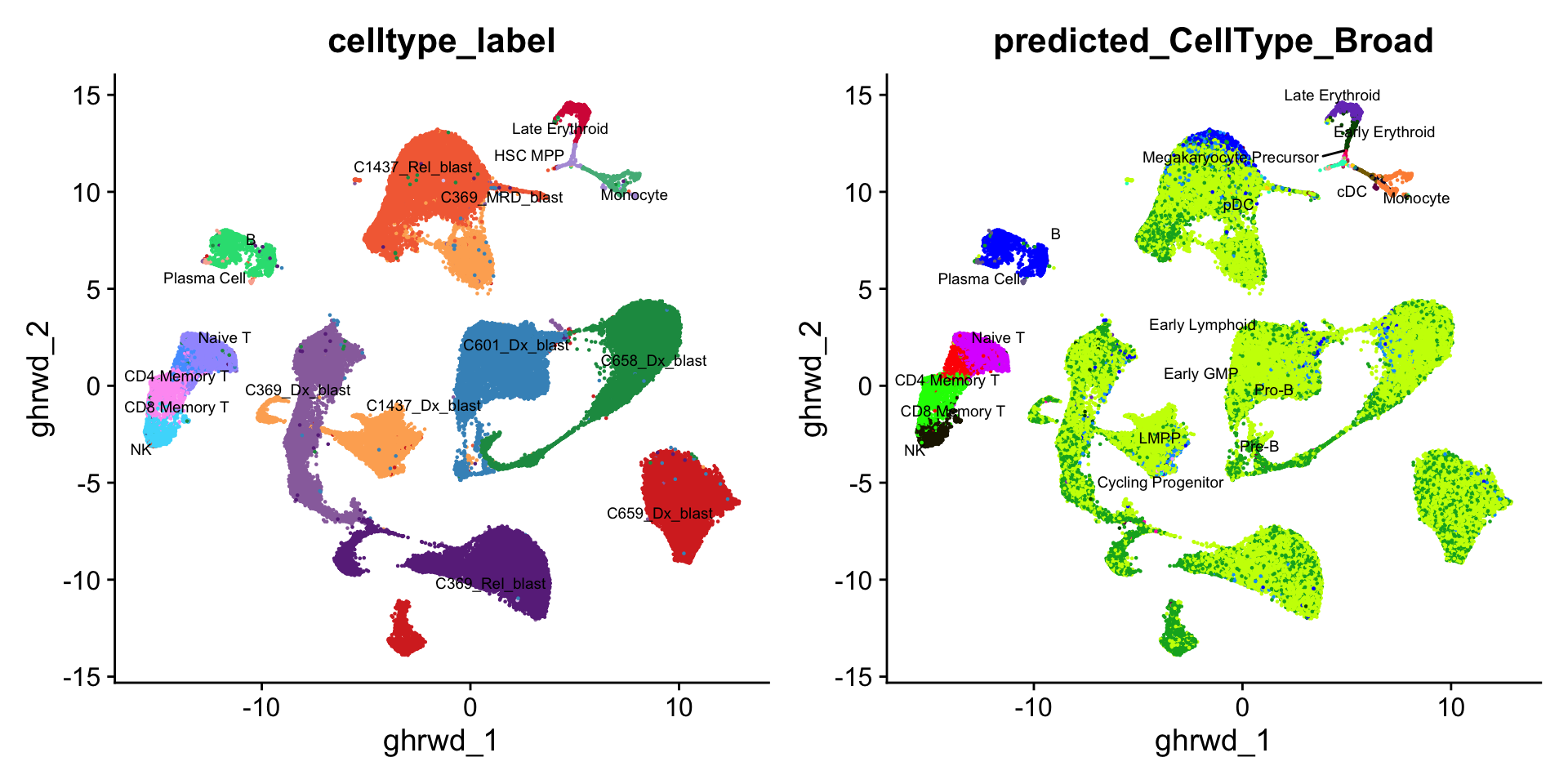
Summary figure
Fusion detection is summarised across all eight samples in narrative order: the three solo diagnosis patients (C601, C658, C659) first to establish baseline detection rates, followed by C1437 (diagnosis and relapse) and C369 (diagnosis, relapse, MRD). For each sample the number of fusion-positive cells and the percentage of all recovered cells is shown. C1437 cells are detected with the v1 probe; all other patients use the v2 probe.
markers <- c(
  # B lineage / blast markers
  "CD19", "CD79A", "DNTT", "MME", "VPREB1",
  # T / NK
  "CD3E", "CD8A", "CD4", "NKG7", "GNLY",
  # Myeloid / monocyte
  "CD14", "S100A8",
  # pDC / plasma
  "IL3RA", "MZB1",
  # Erythroid / progenitor
  "HBB", "GYPA", "CD34"
)

# Lineage-ordered cell type levels for consistent ordering across all panels
lineage_order <- c(
  # B-ALL blasts (ordered by patient then timepoint)
  "C1437_Dx_blast", "C1437_Rel_blast",
  "C369_Dx_blast",  "C369_MRD_blast", "C369_Rel_blast",
  "C601_Dx_blast",
  "C658_Dx_blast",  "C659_Dx_blast",
  # Normal B lineage
  "B", "Plasma Cell",
  # T / NK
  "Naive T", "CD4 Memory T", "CD8 Memory T", "NK",
  # Myeloid
  "Monocyte",
  # Erythroid / progenitor
  "HSC MPP", "Late Erythroid"
)
seu$celltype_label <- factor(seu$celltype_label, levels = lineage_order)

# Corner UMAP arrow annotation (bottom-left)
umap_arrow <- annotation_custom(
  grob = grid::grobTree(
    grid::segmentsGrob(
      x0 = 0.05, y0 = 0.05, x1 = 0.16, y1 = 0.05,
      arrow = grid::arrow(length = grid::unit(0.15, "cm"), type = "closed"),
      gp = grid::gpar(fill = "grey20", col = "grey20", lwd = 2.5)
    ),
    grid::segmentsGrob(
      x0 = 0.05, y0 = 0.05, x1 = 0.05, y1 = 0.16,
      arrow = grid::arrow(length = grid::unit(0.15, "cm"), type = "closed"),
      gp = grid::gpar(fill = "grey20", col = "grey20", lwd = 2.5)
    ),
    grid::textGrob("UMAP", x = 0.105, y = 0.01,
      gp = grid::gpar(fontsize = 8, col = "grey20", fontface = "bold"))
  )
)

umap_theme <- theme_classic() +
  theme(
    axis.line    = element_blank(),
    axis.text    = element_blank(),
    axis.ticks   = element_blank(),
    axis.title   = element_blank(),
    plot.margin  = margin(t = 2, r = 2, b = 2, l = 2)
  )

# --- p1: celltype label UMAP — labels with white halo, no legend ---
# Build centroids manually to pass bg.color/bg.r to geom_text_repel
p1_embed <- as.data.frame(Embeddings(seu, "umap"))
colnames(p1_embed) <- c("UMAP_1", "UMAP_2")
p1_embed$celltype_label <- as.character(seu$celltype_label)

p1_centroids <- p1_embed %>%
  filter(!is.na(celltype_label)) %>%
  group_by(celltype_label) %>%
  summarise(UMAP_1 = median(UMAP_1), UMAP_2 = median(UMAP_2), .groups = "drop")

p1 <- DimPlot(seu, reduction = "umap", label = FALSE,
              group.by = "celltype_label") +
  scale_color_manual(values = celltype_colors, breaks = lineage_order, name = NULL) +
  ggtitle(NULL) +
  ggrepel::geom_text_repel(
    data         = p1_centroids,
    aes(x = UMAP_1, y = UMAP_2, label = celltype_label),
    inherit.aes  = FALSE,
    size         = 3,
    colour       = "black",
    fontface     = "bold",
    bg.color     = adjustcolor("white", alpha.f = 0.5),
    bg.r         = 0.1,
    segment.size = 0.3,
    max.overlaps = Inf,
    seed         = 42
  ) +
  coord_cartesian(clip = "off") +
  umap_theme +
  umap_arrow +
  theme(legend.position = "none")

# --- p2: 2-colour ETV6::RUNX1 fusion highlight ---
umap_coords <- as.data.frame(Embeddings(seu, "umap"))
colnames(umap_coords) <- c("UMAP_1", "UMAP_2")
umap_coords$fusion_label <- dplyr::case_when(
  seu$patient_fusion == "ETV6-RUNX1-v1-fusion" ~ "ETV6::RUNX1-v1",
  seu$patient_fusion == "ETV6-RUNX1-v2-fusion" ~ "ETV6::RUNX1-v2",
  TRUE ~ "Not detected"
)
# Plot not-detected cells first so fusion+ cells are drawn on top
umap_coords <- umap_coords %>%
  arrange(desc(fusion_label == "Not detected"))
umap_coords$fusion_label <- factor(
  umap_coords$fusion_label,
  levels = c("ETV6::RUNX1-v1", "ETV6::RUNX1-v2", "Not detected")
)

p2 <- ggplot(umap_coords, aes(x = UMAP_1, y = UMAP_2, colour = fusion_label)) +
  geom_point(size = 0.3, alpha = 0.8) +
  # Invisible NA points to force all three legend entries to appear
  geom_point(
    data = data.frame(
      UMAP_1 = rep(NA_real_, 3), UMAP_2 = rep(NA_real_, 3),
      fusion_label = factor(
        c("ETV6::RUNX1-v1", "ETV6::RUNX1-v2", "Not detected"),
        levels = c("ETV6::RUNX1-v1", "ETV6::RUNX1-v2", "Not detected")
      )
    ),
    aes(colour = fusion_label), size = 3
  ) +
  scale_colour_manual(
    values = c(
      "ETV6::RUNX1-v1" = "#E69F00",
      "ETV6::RUNX1-v2" = "#0072B2",
      "Not detected" = "grey88"
    ),
    breaks = c("ETV6::RUNX1-v1", "ETV6::RUNX1-v2", "Not detected"),
    drop = FALSE,
    name = NULL
  ) +
  guides(colour = guide_legend(
    nrow = 1,
    override.aes = list(size = 3, alpha = 1)
  )) +
  ggtitle(NULL) +
  coord_cartesian(clip = "off") +
  umap_theme +
  theme(
    legend.position   = "bottom",
    legend.margin     = margin(t = 0, r = 0, b = 0, l = 0),
    legend.box.margin = margin(t = -25, r = 0, b = 0, l = 0)
  ) +
  umap_arrow

# --- p3: dot plot of canonical markers, groups in lineage order ---
# Extract data from DotPlot then rebuild with ggplot for faceting + custom labels.
dot_data <- DotPlot(seu, features = markers, group.by = "celltype_label")$data

# Short display names
label_map <- c(
  "C1437_Dx_blast"       = "C1437 Dx",
  "C1437_Rel_blast"      = "C1437 Rel",
  "C369_Dx_blast"        = "C369 Dx",
  "C369_MRD_blast"       = "C369 MRD",
  "C369_Rel_blast"       = "C369 Rel",
  "C601_Dx_blast"        = "C601 Dx",
  "C658_Dx_blast"        = "C658 Dx",
  "C659_Dx_blast"        = "C659 Dx",
  "B"                    = "B",
  "Plasma Cell"          = "Plasma",
  "Naive T"              = "Naive T",
  "CD4 Memory T"         = "CD4 T",
  "CD8 Memory T"         = "CD8 T",
  "NK"                   = "NK",
  "Monocyte"             = "Mono",
  "HSC MPP"              = "HSC MPP",
  "Late Erythroid"       = "Late Ery"
)

blast_groups <- c("C1437_Dx_blast","C1437_Rel_blast",
                  "C369_Dx_blast","C369_MRD_blast","C369_Rel_blast",
                  "C601_Dx_blast","C658_Dx_blast","C659_Dx_blast")

dot_data <- dot_data %>%
  mutate(
    short_label = label_map[as.character(id)],
    short_label = factor(short_label, levels = rev(label_map))
  )

# Compute lineage group boundaries dynamically from whichever labels are
# actually present in dot_data (robust to empty factor levels being dropped)
lineage_of <- c(
  setNames(rep("Blast", length(blast_groups)), unname(label_map[blast_groups])),
  "B"        = "Normal B", "Plasma"   = "Normal B",
  "Naive T"  = "T/NK",     "CD4 T"    = "T/NK",
  "CD8 T"    = "T/NK",     "NK"       = "T/NK",
  "Mono"     = "Myeloid",
  "HSC MPP"  = "Erythroid", "Late Ery" = "Erythroid"
)
present_levels     <- levels(droplevels(dot_data$short_label))
groups_present     <- lineage_of[present_levels]
lineage_boundaries <- which(groups_present[-1] != groups_present[-length(groups_present)]) + 0.5

p3 <- ggplot(dot_data, aes(x = short_label, y = features.plot,
                            colour = avg.exp.scaled, size = pct.exp)) +
  geom_point() +
  geom_vline(xintercept = lineage_boundaries,
             linetype = "dotted", colour = "grey50", linewidth = 0.4) +
  scale_colour_distiller(palette = "Purples", direction = 1,
                         name = "Avg. expr.\n(scaled)") +
  scale_size_continuous(range = c(0, 5), name = "% expressed",
                        breaks = c(0, 25, 50, 75, 100)) +
  coord_flip() +
  labs(x = NULL, y = NULL) +
  theme_classic(base_size = 10) +
  theme(
    axis.text.x     = element_text(angle = 45, hjust = 1, size = 7),
    # Factor levels run bottom-to-top: normal first (12), then blasts (8)
    axis.text.y     = element_text(
      size = 7.5,
      face = c(rep("plain", length(label_map) - length(blast_groups)),
               rep("bold", length(blast_groups)))
    ),
    legend.position = "right",
    legend.box      = "vertical",
    legend.title    = element_text(size = 8),
    legend.text     = element_text(size = 7),
    plot.margin     = margin(t = 5, r = 5, b = 5, l = 5)
  )

# --- p4: per-sample % fusion-positive cells, faceted by capture ---
sample_order <- c(
  "C1437_Diagnosis", "C1437_Relapse",
  "C659_Diagnosis",  "C369_Diagnosis",
  "C369_MRD",        "C369_Relapse",
  "C658_Diagnosis",  "C601_Diagnosis"
)

sample_labels <- c(
  "C601_Diagnosis"  = "C601 Dx",  "C658_Diagnosis"  = "C658 Dx",
  "C659_Diagnosis"  = "C659 Dx",  "C1437_Diagnosis" = "C1437 Dx",
  "C1437_Relapse"   = "C1437 Rel","C369_Diagnosis"  = "C369 Dx",
  "C369_Relapse"    = "C369 Rel", "C369_MRD"        = "C369 MRD"
)

capture_map <- c(
  "C659_Diagnosis"  = "Capture 1", "C1437_Diagnosis" = "Capture 1",
  "C1437_Relapse"   = "Capture 1", "C369_Diagnosis"  = "Capture 1",
  "C601_Diagnosis"  = "Capture 2", "C658_Diagnosis"  = "Capture 2",
  "C369_MRD"        = "Capture 2", "C369_Relapse"    = "Capture 2"
)

sample_colours <- c(
  "C1437 Dx"  = "#FDAE61", "C1437 Rel" = "#F46D43",
  "C659 Dx"   = "#D73027", "C369 Dx"   = "#9970AB",
  "C369 MRD"  = "#DEC9E9", "C369 Rel"  = "#6A2E8A",
  "C658 Dx"   = "#1A9850", "C601 Dx"   = "#4393C3"
)

fusion_summary <- seu@meta.data %>%
  filter(patient_timepoint %in% sample_order) %>%
  mutate(
    fusion_detected = dplyr::case_when(
      patient_timepoint %in% c("C1437_Diagnosis", "C1437_Relapse") ~
        patient_fusion == "ETV6-RUNX1-v1-fusion",
      TRUE ~
        patient_fusion == "ETV6-RUNX1-v2-fusion"
    ),
    is_blast = str_detect(as.character(celltype_label), "_blast"),
    capture  = factor(capture_map[as.character(patient_timepoint)],
                      levels = c("Capture 1", "Capture 2")),
    sample   = factor(patient_timepoint, levels = sample_order,
                      labels = sample_labels[sample_order])
  ) %>%
  group_by(sample, capture) %>%
  summarise(
    total        = n(),
    n_fusion     = sum(fusion_detected),
    pct_of_total = n_fusion / total * 100,
    .groups      = "drop"
  ) %>%
  mutate(pct_label = paste0(round(pct_of_total, 1), "%"))

capture_medians <- fusion_summary %>%
  group_by(capture) %>%
  summarise(median_pct = median(pct_of_total), .groups = "drop")

p4 <- ggplot(fusion_summary,
             aes(x = sample, y = pct_of_total, fill = sample)) +
  geom_col(width = 0.8) +
  geom_text(aes(label = pct_label), vjust = -0.4, size = 2.5) +
  geom_hline(data = capture_medians, aes(yintercept = median_pct),
             linetype = "dashed", colour = "grey40", linewidth = 0.5) +
  scale_fill_manual(values = sample_colours, guide = "none") +
  scale_y_continuous(expand = expansion(mult = c(0, 0.15)),
                     breaks = seq(0, 60, 20),
                     name   = "Fusion-positive cells (%)") +
  scale_x_discrete(name = NULL) +
  facet_wrap(~ capture, scales = "free_x", nrow = 1) +
  theme_classic(base_size = 10) +
  theme(
    axis.text.x        = element_text(angle = 45, hjust = 1, size = 8),
    panel.grid.major.y = element_line(colour = "grey92", linewidth = 0.3),
    strip.background   = element_blank(),
    strip.text         = element_text(size = 9, face = "plain")
  )

(p1 | p2 | p3 | p4) + plot_layout(widths = c(2, 2, 2.5, 1.5))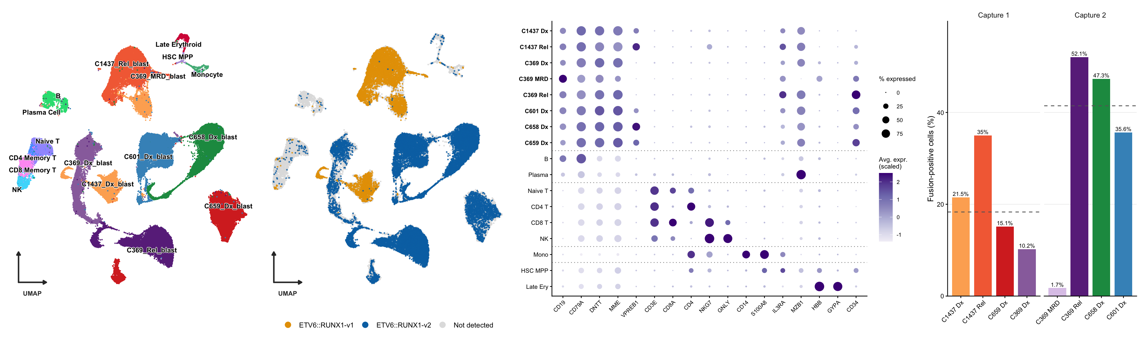
Session info
sessioninfo::session_info()─ Session info ───────────────────────────────────────────────────────────────
setting value
version R version 4.4.1 (2024-06-14)
os macOS 15.5
system aarch64, darwin20
ui X11
language (EN)
collate en_US.UTF-8
ctype en_US.UTF-8
tz Australia/Melbourne
date 2026-07-16
pandoc 3.8.3 @ /Applications/RStudio.app/Contents/Resources/app/quarto/bin/tools/aarch64/ (via rmarkdown)
quarto 1.9.38 @ /Applications/RStudio.app/Contents/Resources/app/quarto/bin/quarto
─ Packages ───────────────────────────────────────────────────────────────────
! package * version date (UTC) lib source
P abind 1.4-8 2024-09-12 [?] CRAN (R 4.4.1)
P backports 1.5.0 2024-05-23 [?] CRAN (R 4.4.1)
P Biobase 2.66.0 2024-11-08 [?] Bioconduc~
P BiocGenerics 0.52.0 2024-11-08 [?] Bioconduc~
P BiocManager 1.30.27 2025-11-14 [?] CRAN (R 4.4.3)
P bslib 0.9.0 2025-01-30 [?] CRAN (R 4.4.1)
P cachem 1.1.0 2024-05-16 [?] CRAN (R 4.4.1)
P callr 3.7.6 2024-03-25 [?] CRAN (R 4.4.0)
P checkmate 2.3.2 2024-07-29 [?] CRAN (R 4.4.0)
P cli 3.6.5 2025-04-23 [?] CRAN (R 4.4.1)
P cluster 2.1.6 2023-12-01 [?] CRAN (R 4.4.1)
P clustree * 0.5.1 2023-11-05 [?] CRAN (R 4.4.0)
P codetools 0.2-20 2024-03-31 [?] CRAN (R 4.4.1)
P colorspace 2.1-1 2024-07-26 [?] CRAN (R 4.4.1)
P cowplot 1.1.3 2024-01-22 [?] CRAN (R 4.4.0)
P crayon 1.5.3 2024-06-20 [?] CRAN (R 4.4.1)
P data.table 1.18.2.1 2026-01-27 [?] CRAN (R 4.4.3)
P DelayedArray 0.32.0 2024-11-08 [?] Bioconduc~
P deldir 2.0-4 2024-02-28 [?] CRAN (R 4.4.1)
P digest 0.6.37 2024-08-19 [?] CRAN (R 4.4.1)
P dotCall64 1.2 2024-10-04 [?] CRAN (R 4.4.1)
P dplyr * 1.1.4 2023-11-17 [?] CRAN (R 4.4.0)
P evaluate 1.0.3 2025-01-10 [?] CRAN (R 4.4.1)
P farver 2.1.2 2024-05-13 [?] CRAN (R 4.4.1)
P fastDummies 1.7.5 2025-01-20 [?] CRAN (R 4.4.1)
P fastmap 1.2.0 2024-05-15 [?] CRAN (R 4.4.1)
P fitdistrplus 1.2-2 2025-01-07 [?] CRAN (R 4.4.1)
P forcats * 1.0.0 2023-01-29 [?] CRAN (R 4.4.0)
P fs 1.6.6 2025-04-12 [?] CRAN (R 4.4.1)
P future 1.49.0 2025-05-09 [?] CRAN (R 4.4.1)
P future.apply 1.11.3 2024-10-27 [?] CRAN (R 4.4.1)
P generics 0.1.4 2025-05-09 [?] CRAN (R 4.4.1)
P GenomeInfoDb 1.42.3 2025-01-27 [?] Bioconduc~
P GenomeInfoDbData 1.2.13 2025-05-28 [?] Bioconductor
P GenomicRanges 1.58.0 2024-11-08 [?] Bioconduc~
P getPass 0.2-4 2023-12-10 [?] CRAN (R 4.4.1)
P ggforce 0.4.2 2024-02-19 [?] CRAN (R 4.4.0)
P ggplot2 * 4.0.2 2026-02-03 [?] CRAN (R 4.4.3)
P ggraph * 2.2.1 2024-03-07 [?] CRAN (R 4.4.0)
P ggrepel * 0.9.6 2024-09-07 [?] CRAN (R 4.4.1)
P ggridges 0.5.6 2024-01-23 [?] CRAN (R 4.4.0)
P git2r 0.36.2 2025-03-29 [?] CRAN (R 4.4.1)
P glmGamPoi * 1.18.0 2024-11-08 [?] Bioconduc~
P globals 0.18.0 2025-05-08 [?] CRAN (R 4.4.1)
P glue * 1.8.0 2024-09-30 [?] CRAN (R 4.4.1)
P goftest 1.2-3 2021-10-07 [?] CRAN (R 4.4.1)
P graphlayouts 1.2.2 2025-01-23 [?] CRAN (R 4.4.1)
P gridExtra 2.3 2017-09-09 [?] CRAN (R 4.4.1)
P gtable 0.3.6 2024-10-25 [?] CRAN (R 4.4.1)
P here * 1.0.1 2020-12-13 [?] CRAN (R 4.4.1)
P hms 1.1.3 2023-03-21 [?] CRAN (R 4.4.0)
P htmltools 0.5.8.1 2024-04-04 [?] CRAN (R 4.4.1)
P htmlwidgets 1.6.4 2023-12-06 [?] CRAN (R 4.4.0)
P httpuv 1.6.16 2025-04-16 [?] CRAN (R 4.4.1)
P httr 1.4.7 2023-08-15 [?] CRAN (R 4.4.0)
P ica 1.0-3 2022-07-08 [?] CRAN (R 4.4.1)
P igraph 2.1.4 2025-01-23 [?] CRAN (R 4.4.1)
P IRanges 2.40.1 2024-12-05 [?] Bioconduc~
P irlba 2.3.5.1 2022-10-03 [?] CRAN (R 4.4.0)
P jquerylib 0.1.4 2021-04-26 [?] CRAN (R 4.4.0)
P jsonlite 2.0.0 2025-03-27 [?] CRAN (R 4.4.1)
P KernSmooth 2.23-24 2024-05-17 [?] CRAN (R 4.4.1)
P knitr 1.50 2025-03-16 [?] CRAN (R 4.4.1)
P labeling 0.4.3 2023-08-29 [?] CRAN (R 4.4.1)
P later 1.4.2 2025-04-08 [?] CRAN (R 4.4.1)
P lattice 0.22-6 2024-03-20 [?] CRAN (R 4.4.1)
P lazyeval 0.2.2 2019-03-15 [?] CRAN (R 4.4.1)
P leidenbase 0.1.35 2025-04-02 [?] CRAN (R 4.4.1)
P lifecycle 1.0.4 2023-11-07 [?] CRAN (R 4.4.1)
P listenv 0.9.1 2024-01-29 [?] CRAN (R 4.4.1)
P lmtest 0.9-40 2022-03-21 [?] CRAN (R 4.4.1)
P lubridate * 1.9.4 2024-12-08 [?] CRAN (R 4.4.1)
P magrittr 2.0.3 2022-03-30 [?] CRAN (R 4.4.1)
P MASS 7.3-60.2 2024-04-26 [?] CRAN (R 4.4.1)
P Matrix 1.7-0 2024-04-26 [?] CRAN (R 4.4.1)
P MatrixGenerics 1.18.1 2025-01-09 [?] Bioconduc~
P matrixStats 1.5.0 2025-01-07 [?] CRAN (R 4.4.1)
P memoise 2.0.1 2021-11-26 [?] CRAN (R 4.4.0)
P mime 0.13 2025-03-17 [?] CRAN (R 4.4.1)
P miniUI 0.1.2 2025-04-17 [?] CRAN (R 4.4.1)
P nlme 3.1-164 2023-11-27 [?] CRAN (R 4.4.1)
P paletteer 1.6.0 2024-01-21 [?] CRAN (R 4.4.0)
P parallelly 1.45.0 2025-06-02 [?] CRAN (R 4.4.1)
P patchwork * 1.3.0 2024-09-16 [?] CRAN (R 4.4.1)
P pbapply 1.7-4 2025-07-20 [?] CRAN (R 4.4.1)
P pillar 1.10.2 2025-04-05 [?] CRAN (R 4.4.1)
P pkgconfig 2.0.3 2019-09-22 [?] CRAN (R 4.4.1)
P plotly 4.10.4 2024-01-13 [?] CRAN (R 4.4.0)
P plyr 1.8.9 2023-10-02 [?] CRAN (R 4.4.1)
P png 0.1-8 2022-11-29 [?] CRAN (R 4.4.1)
P polyclip 1.10-7 2024-07-23 [?] CRAN (R 4.4.1)
P prismatic 1.1.2 2024-04-10 [?] CRAN (R 4.4.1)
P processx 3.8.6 2025-02-21 [?] CRAN (R 4.4.1)
P progressr 0.15.1 2024-11-22 [?] CRAN (R 4.4.1)
P promises 1.3.3 2025-05-29 [?] CRAN (R 4.4.1)
P ps 1.9.1 2025-04-12 [?] CRAN (R 4.4.1)
P purrr * 1.0.4 2025-02-05 [?] CRAN (R 4.4.1)
P R6 2.6.1 2025-02-15 [?] CRAN (R 4.4.1)
P RANN 2.6.2 2024-08-25 [?] CRAN (R 4.4.1)
P RColorBrewer 1.1-3 2022-04-03 [?] CRAN (R 4.4.1)
P Rcpp 1.1.1-1.1 2026-04-24 [?] CRAN (R 4.4.1)
P RcppAnnoy 0.0.22 2024-01-23 [?] CRAN (R 4.4.1)
P RcppHNSW 0.6.0 2024-02-04 [?] CRAN (R 4.4.1)
P readr * 2.1.5 2024-01-10 [?] CRAN (R 4.4.0)
P rematch2 2.1.2 2020-05-01 [?] CRAN (R 4.4.0)
renv 1.1.4 2025-03-20 [1] CRAN (R 4.4.1)
P reshape2 1.4.4 2020-04-09 [?] CRAN (R 4.4.0)
P reticulate 1.42.0 2025-03-25 [?] CRAN (R 4.4.1)
P rlang 1.1.6 2025-04-11 [?] CRAN (R 4.4.1)
P rmarkdown 2.29 2024-11-04 [?] CRAN (R 4.4.1)
P ROCR 1.0-11 2020-05-02 [?] CRAN (R 4.4.0)
P rprojroot 2.0.4 2023-11-05 [?] CRAN (R 4.4.1)
P RSpectra 0.16-2 2024-07-18 [?] CRAN (R 4.4.0)
P rstudioapi 0.17.1 2024-10-22 [?] CRAN (R 4.4.1)
P Rtsne 0.17 2023-12-07 [?] CRAN (R 4.4.1)
P S4Arrays 1.6.0 2024-11-08 [?] Bioconduc~
P S4Vectors 0.44.0 2024-11-08 [?] Bioconduc~
P S7 0.2.0 2024-11-07 [?] CRAN (R 4.4.1)
P sass 0.4.10 2025-04-11 [?] CRAN (R 4.4.1)
P scales * 1.4.0 2025-04-24 [?] CRAN (R 4.4.1)
P scattermore 1.2 2023-06-12 [?] CRAN (R 4.4.0)
P sctransform 0.4.2 2025-04-30 [?] CRAN (R 4.4.1)
P sessioninfo 1.2.3 2025-02-05 [?] CRAN (R 4.4.1)
P Seurat * 5.3.0 2025-04-23 [?] CRAN (R 4.4.1)
P SeuratObject * 5.1.0 2025-04-22 [?] CRAN (R 4.4.1)
P shiny 1.10.0 2024-12-14 [?] CRAN (R 4.4.1)
P sp * 2.2-0 2025-02-01 [?] CRAN (R 4.4.1)
P spam 2.11-1 2025-01-20 [?] CRAN (R 4.4.1)
P SparseArray 1.6.2 2025-02-20 [?] Bioconduc~
P spatstat.data 3.1-6 2025-03-17 [?] CRAN (R 4.4.1)
P spatstat.explore 3.4-3 2025-05-21 [?] CRAN (R 4.4.1)
P spatstat.geom 3.4-1 2025-05-20 [?] CRAN (R 4.4.1)
P spatstat.random 3.4-1 2025-05-20 [?] CRAN (R 4.4.1)
P spatstat.sparse 3.1-0 2024-06-21 [?] CRAN (R 4.4.0)
P spatstat.univar 3.1-3 2025-05-08 [?] CRAN (R 4.4.1)
P spatstat.utils 3.1-4 2025-05-15 [?] CRAN (R 4.4.1)
P stringi 1.8.7 2025-03-27 [?] CRAN (R 4.4.1)
P stringr * 1.6.0 2025-11-04 [?] CRAN (R 4.4.1)
P SummarizedExperiment 1.36.0 2024-11-08 [?] Bioconduc~
P survival 3.6-4 2024-04-24 [?] CRAN (R 4.4.1)
P tensor 1.5 2012-05-05 [?] CRAN (R 4.4.1)
P tibble * 3.2.1 2023-03-20 [?] CRAN (R 4.4.0)
P tidygraph 1.3.1 2024-01-30 [?] CRAN (R 4.4.0)
P tidyr * 1.3.1 2024-01-24 [?] CRAN (R 4.4.1)
P tidyselect 1.2.1 2024-03-11 [?] CRAN (R 4.4.0)
P tidyverse * 2.0.0 2023-02-22 [?] CRAN (R 4.4.0)
P timechange 0.3.0 2024-01-18 [?] CRAN (R 4.4.1)
P tweenr 2.0.3 2024-02-26 [?] CRAN (R 4.4.0)
P tzdb 0.5.0 2025-03-15 [?] CRAN (R 4.4.1)
P UCSC.utils 1.2.0 2024-11-08 [?] Bioconduc~
P utf8 1.2.5 2025-05-01 [?] CRAN (R 4.4.1)
P uwot 0.2.3 2025-02-24 [?] CRAN (R 4.4.1)
P vctrs 0.6.5 2023-12-01 [?] CRAN (R 4.4.0)
P viridis 0.6.5 2024-01-29 [?] CRAN (R 4.4.0)
P viridisLite 0.4.2 2023-05-02 [?] CRAN (R 4.4.1)
P whisker 0.4.1 2022-12-05 [?] CRAN (R 4.4.1)
P withr 3.0.2 2024-10-28 [?] CRAN (R 4.4.1)
P workflowr * 1.7.1 2023-08-23 [?] CRAN (R 4.4.0)
P xfun 0.56 2026-01-18 [?] CRAN (R 4.4.3)
P xtable 1.8-4 2019-04-21 [?] CRAN (R 4.4.1)
P XVector 0.46.0 2024-11-08 [?] Bioconduc~
P yaml 2.3.10 2024-07-26 [?] CRAN (R 4.4.1)
P zlibbioc 1.52.0 2024-11-08 [?] Bioconduc~
P zoo 1.8-14 2025-04-10 [?] CRAN (R 4.4.1)
[1] /Users/maksimovicjovana/projects/active/flex-fusion-probes/renv/library/macos/R-4.4/aarch64-apple-darwin20
[2] /Users/maksimovicjovana/Library/Caches/org.R-project.R/R/renv/sandbox/macos/R-4.4/aarch64-apple-darwin20/f7156815
* ── Packages attached to the search path.
P ── Loaded and on-disk path mismatch.
──────────────────────────────────────────────────────────────────────────────
sessionInfo()R version 4.4.1 (2024-06-14)
Platform: aarch64-apple-darwin20
Running under: macOS 15.5
Matrix products: default
BLAS: /Library/Frameworks/R.framework/Versions/4.4-arm64/Resources/lib/libRblas.0.dylib
LAPACK: /Library/Frameworks/R.framework/Versions/4.4-arm64/Resources/lib/libRlapack.dylib; LAPACK version 3.12.0
locale:
[1] en_US.UTF-8/en_US.UTF-8/en_US.UTF-8/C/en_US.UTF-8/en_US.UTF-8
time zone: Australia/Melbourne
tzcode source: internal
attached base packages:
[1] stats graphics grDevices datasets utils methods base
other attached packages:
[1] ggrepel_0.9.6 glmGamPoi_1.18.0 clustree_0.5.1 ggraph_2.2.1
[5] patchwork_1.3.0 scales_1.4.0 Seurat_5.3.0 SeuratObject_5.1.0
[9] sp_2.2-0 glue_1.8.0 here_1.0.1 lubridate_1.9.4
[13] forcats_1.0.0 stringr_1.6.0 dplyr_1.1.4 purrr_1.0.4
[17] readr_2.1.5 tidyr_1.3.1 tibble_3.2.1 ggplot2_4.0.2
[21] tidyverse_2.0.0 workflowr_1.7.1
loaded via a namespace (and not attached):
[1] RcppAnnoy_0.0.22 splines_4.4.1
[3] later_1.4.2 prismatic_1.1.2
[5] polyclip_1.10-7 fastDummies_1.7.5
[7] lifecycle_1.0.4 rprojroot_2.0.4
[9] globals_0.18.0 processx_3.8.6
[11] lattice_0.22-6 MASS_7.3-60.2
[13] backports_1.5.0 magrittr_2.0.3
[15] plotly_4.10.4 sass_0.4.10
[17] rmarkdown_2.29 jquerylib_0.1.4
[19] yaml_2.3.10 httpuv_1.6.16
[21] sctransform_0.4.2 spam_2.11-1
[23] sessioninfo_1.2.3 spatstat.sparse_3.1-0
[25] reticulate_1.42.0 cowplot_1.1.3
[27] pbapply_1.7-4 RColorBrewer_1.1-3
[29] abind_1.4-8 zlibbioc_1.52.0
[31] Rtsne_0.17 GenomicRanges_1.58.0
[33] BiocGenerics_0.52.0 tweenr_2.0.3
[35] git2r_0.36.2 GenomeInfoDbData_1.2.13
[37] IRanges_2.40.1 S4Vectors_0.44.0
[39] irlba_2.3.5.1 listenv_0.9.1
[41] spatstat.utils_3.1-4 goftest_1.2-3
[43] RSpectra_0.16-2 spatstat.random_3.4-1
[45] fitdistrplus_1.2-2 parallelly_1.45.0
[47] codetools_0.2-20 DelayedArray_0.32.0
[49] ggforce_0.4.2 tidyselect_1.2.1
[51] UCSC.utils_1.2.0 farver_2.1.2
[53] viridis_0.6.5 matrixStats_1.5.0
[55] stats4_4.4.1 spatstat.explore_3.4-3
[57] jsonlite_2.0.0 tidygraph_1.3.1
[59] progressr_0.15.1 ggridges_0.5.6
[61] survival_3.6-4 tools_4.4.1
[63] ica_1.0-3 Rcpp_1.1.1-1.1
[65] SparseArray_1.6.2 gridExtra_2.3
[67] xfun_0.56 MatrixGenerics_1.18.1
[69] GenomeInfoDb_1.42.3 withr_3.0.2
[71] BiocManager_1.30.27 fastmap_1.2.0
[73] callr_3.7.6 digest_0.6.37
[75] timechange_0.3.0 R6_2.6.1
[77] mime_0.13 colorspace_2.1-1
[79] scattermore_1.2 tensor_1.5
[81] spatstat.data_3.1-6 utf8_1.2.5
[83] generics_0.1.4 renv_1.1.4
[85] data.table_1.18.2.1 graphlayouts_1.2.2
[87] httr_1.4.7 htmlwidgets_1.6.4
[89] S4Arrays_1.6.0 whisker_0.4.1
[91] uwot_0.2.3 pkgconfig_2.0.3
[93] gtable_0.3.6 lmtest_0.9-40
[95] S7_0.2.0 XVector_0.46.0
[97] htmltools_0.5.8.1 dotCall64_1.2
[99] Biobase_2.66.0 png_0.1-8
[101] spatstat.univar_3.1-3 knitr_1.50
[103] rstudioapi_0.17.1 tzdb_0.5.0
[105] reshape2_1.4.4 checkmate_2.3.2
[107] nlme_3.1-164 cachem_1.1.0
[109] zoo_1.8-14 KernSmooth_2.23-24
[111] parallel_4.4.1 miniUI_0.1.2
[113] pillar_1.10.2 grid_4.4.1
[115] vctrs_0.6.5 RANN_2.6.2
[117] promises_1.3.3 xtable_1.8-4
[119] cluster_2.1.6 paletteer_1.6.0
[121] evaluate_1.0.3 cli_3.6.5
[123] compiler_4.4.1 rlang_1.1.6
[125] crayon_1.5.3 leidenbase_0.1.35
[127] future.apply_1.11.3 labeling_0.4.3
[129] rematch2_2.1.2 ps_1.9.1
[131] getPass_0.2-4 plyr_1.8.9
[133] fs_1.6.6 stringi_1.8.7
[135] viridisLite_0.4.2 deldir_2.0-4
[137] lazyeval_0.2.2 spatstat.geom_3.4-1
[139] Matrix_1.7-0 RcppHNSW_0.6.0
[141] hms_1.1.3 future_1.49.0
[143] shiny_1.10.0 SummarizedExperiment_1.36.0
[145] ROCR_1.0-11 igraph_2.1.4
[147] memoise_2.0.1 bslib_0.9.0