B-ALL Experiment 2: Non-blast Fusion Analysis
ETV6::RUNX1 detections in non-blast cells across Exp2 — evidence for a pre-leukaemic progenitor clone
2026-07-16
Last updated: 2026-07-16
Checks: 6 1
Knit directory: flex-fusion-probes/
This reproducible R Markdown analysis was created with workflowr (version 1.7.1). The Checks tab describes the reproducibility checks that were applied when the results were created. The Past versions tab lists the development history.
Great! Since the R Markdown file has been committed to the Git repository, you know the exact version of the code that produced these results.
Great job! The global environment was empty. Objects defined in the global environment can affect the analysis in your R Markdown file in unknown ways. For reproduciblity it’s best to always run the code in an empty environment.
The command set.seed(20240925) was run prior to running
the code in the R Markdown file. Setting a seed ensures that any results
that rely on randomness, e.g. subsampling or permutations, are
reproducible.
Great job! Recording the operating system, R version, and package versions is critical for reproducibility.
- estimate-ambient
To ensure reproducibility of the results, delete the cache directory
B-ALL_exp2_nonblast_fusion_analysis_cache and re-run the
analysis. To have workflowr automatically delete the cache directory
prior to building the file, set delete_cache = TRUE when
running wflow_build() or wflow_publish().
Great job! Using relative paths to the files within your workflowr project makes it easier to run your code on other machines.
Great! You are using Git for version control. Tracking code development and connecting the code version to the results is critical for reproducibility.
The results in this page were generated with repository version 94f7541. See the Past versions tab to see a history of the changes made to the R Markdown and HTML files.
Note that you need to be careful to ensure that all relevant files for
the analysis have been committed to Git prior to generating the results
(you can use wflow_publish or
wflow_git_commit). workflowr only checks the R Markdown
file, but you know if there are other scripts or data files that it
depends on. Below is the status of the Git repository when the results
were generated:
Ignored files:
    Ignored:    .DS_Store
    Ignored:    .Rhistory
    Ignored:    .Rproj.user/
    Ignored:    analysis/.gitignore
    Ignored:    analysis/B-ALL_exp2_nonblast_fusion_analysis_cache/
    Ignored:    analysis/figure/
    Ignored:    analysis/obsolete/B-ALL_nonblast_fusion_analysis_cache/
    Ignored:    analysis/projectionFigures/
    Ignored:    code/files/
    Ignored:    data/.DS_Store
    Ignored:    data/BoneMarrowMap/
    Ignored:    data/BoneMarrowMapBoneMarrowMap_SymphonyReference.rds
    Ignored:    data/BoneMarrowMapBoneMarrowMap_uwot_model.uwot
    Ignored:    data/CAPTURE-1-POOL-FLEX/
    Ignored:    data/CAPTURE-2-POOL-FLEX/
    Ignored:    data/Pool-240917-FLEX/
    Ignored:    data/RDS/
    Ignored:    data/Run_1_and_Run_2/
    Ignored:    data/Run_2/
    Ignored:    logs/
    Ignored:    output/
    Ignored:    projectionFigures/
    Ignored:    renv/library/
    Ignored:    renv/staging/

Untracked files:
    Untracked:  CLAUDE.md
    Untracked:  data/sample_information_flex_experiment_2_table.csv
    Untracked:  poster.pptx

Unstaged changes:
    Deleted:    analysis/B-ALL_exp2_background.Rmd
    Deleted:    analysis/B-ALL_exp2_c1437_li2025_clone_analysis.Rmd
    Deleted:    analysis/B-ALL_nonblast_fusion_analysis.Rmd
    Modified:   render_all.sh
Note that any generated files, e.g. HTML, png, CSS, etc., are not included in this status report because it is ok for generated content to have uncommitted changes.
These are the previous versions of the repository in which changes were
made to the R Markdown
(analysis/B-ALL_exp2_nonblast_fusion_analysis.Rmd) and HTML
(docs/B-ALL_exp2_nonblast_fusion_analysis.html) files. If
you’ve configured a remote Git repository (see
?wflow_git_remote), click on the hyperlinks in the table
below to view the files as they were in that past version.
| File | Version | Author | Date | Message |
|---|---|---|---|---|
| Rmd | 94f7541 | Jovana Maksimovic | 2026-07-16 | wflow_publish("analysis/B-ALL_exp2_nonblast_fusion_analysis.Rmd") |
ETV6::RUNX1 is thought to arise in utero in a multipotent haematopoietic progenitor, establishing a pre-leukaemic clone that can persist for years before acquiring the secondary events required for overt leukaemia (Mori et al. 2002; Ford et al. 1998; Wiemels et al. 1999). Cells descending from this progenitor may differentiate along normal haematopoietic lineages — erythroid, myeloid, T cell, NK — while retaining the fusion as a molecular scar, without undergoing leukaemic transformation.
This notebook characterises ETV6::RUNX1 fusion detections in non-blast cells across Exp2 (eight B-ALL samples, two Flex captures) and asks whether they are consistent with genuine expression in pre-leukaemic progenitor progeny or with ambient RNA contamination. The analysis has four components:
- Ambient RNA baseline — estimate fusion transcript concentration in empty droplets (the ambient soup) and confirm that ETV6::RUNX1 ambient levels are very low.
- Non-blast fusion landscape — characterise which cell types carry fusion transcripts, across which patients, and at what UMI levels.
- Blast marker expression — confirm that non-blast fusion-positive cells do not express canonical blast markers (CD19, DNTT, MME, CD34).
- Ambient contamination score — score each cell for overall ambient RNA burden and test whether fusion-positive cells have higher scores than fusion-negative cells of the same type.
suppressPackageStartupMessages({
  library(Seurat)
  library(DropletUtils)
  library(tidyverse)
  library(patchwork)
  library(ggrepel)
  library(here)
  library(glue)
  library(scales)
})

theme_pub <- function(base_size = 11) {
  theme_bw(base_size = base_size) +
    theme(
      panel.grid.minor  = element_blank(),
      strip.background  = element_rect(fill = "grey92", colour = NA),
      legend.key.size   = unit(0.4, "cm"),
      plot.title        = element_text(face = "bold", size = base_size),
      plot.subtitle     = element_text(size = base_size - 1, colour = "grey40")
    )
}

# Strip tnk_ / bm_ prefixes from celltype_label values for display
strip_prefix <- function(x) gsub("^(tnk_|bm_)", "", x)

# Clean fusion labels: ETV6-RUNX1-v2-fusion → ETV6::RUNX1-v2
clean_label <- function(x) {
  stripped <- gsub("-fusion$", "", x)
  parts    <- gsub("-", "::", stripped, fixed = TRUE)
  ifelse(
    grepl("^\\w+::\\w+::v\\d+(::.*)?$", parts),
    sub("^(\\w+::\\w+::v\\d+).*$", "\\1", parts),
    sub("^(\\w+::\\w+)::.*$", "\\1", parts)
  )
}

# Cell type colour palette — colours match B-ALL_exp2_joint_clustering.Rmd
ct_palette <- c(
  "Late Erythroid"       = "#D62246",
  "Early Erythroid"      = "#8C564B",
  "Erythroid Progenitor" = "#C49C94",
  "HSC MPP"              = "#B39DDB",
  "Monocyte"             = "#52B788",
  "pDC"                  = "#9467BD",
  "Naive T"              = "#A29BFE",
  "CD4 Memory T"         = "#54A0FF",
  "CD8 Memory T"         = "#FF9FF3",
  "NK"                   = "#48DBFB",
  "Pro-B"                = "#6BAED6",
  "B"                    = "#1F77B4",
  "Plasma Cell"          = "#756BB1",
  "Other"                = "grey70"
)

ct_order <- c(
  "Late Erythroid", "Early Erythroid", "Erythroid Progenitor",
  "HSC MPP", "Monocyte", "pDC",
  "Naive T", "CD4 Memory T", "CD8 Memory T", "NK",
  "Pro-B", "B", "Plasma Cell",
  "Other"
)

# Sample colour palette — matches Figure 4 (B-ALL_exp2_joint_clustering.Rmd)
sample_palette <- c(
  "C1437_Diagnosis" = "#FDAE61",
  "C1437_Relapse"   = "#F46D43",
  "C659_Diagnosis"  = "#D73027",
  "C369_Diagnosis"  = "#9970AB",
  "C369_MRD"        = "#DEC9E9",
  "C369_Relapse"    = "#6A2E8A",
  "C658_Diagnosis"  = "#1A9850",
  "C601_Diagnosis"  = "#4393C3"
)

patient_fusions <- c("ETV6-RUNX1-v1-fusion", "ETV6-RUNX1-v2-fusion")
Load data
The joint annotated Exp2 object
(exp2_joint_annotated.seu.rds) is used — saved after
BoneMarrowMap annotation in B-ALL_exp2_joint_clustering.Rmd
and containing celltype_label,
patient_timepoint, and Capture.
seu_exp2 <- readRDS(here("data", "RDS", "exp2_joint_annotated.seu.rds"))

cat(glue("Exp2: {ncol(seu_exp2)} cells\n"))
Exp2: 87534 cellscat("\nTop celltype_label values:\n")
Top celltype_label values:print(head(sort(table(seu_exp2$celltype_label), decreasing = TRUE), 15))
C1437_Rel_blast   C659_Dx_blast  C369_Rel_blast   C601_Dx_blast   C369_Dx_blast
          13388           12617           11819           11214           10714
  C658_Dx_blast  C1437_Dx_blast         Naive T               B    CD8 Memory T
          10418            9219            2117            1720            1501
             NK  Late Erythroid        Monocyte    CD4 Memory T         HSC MPP
           1069             560             538             372             203
Define non-blast cells
Blast cells are identified by the _blast pattern in
celltype_label — a cluster-level call that is more robust
than per-cell predicted_CellType_Broad at the blast/normal
boundary, particularly in high-blast-burden samples. A clean,
prefix-stripped version of the label is stored as
cluster_celltype for plotting.
ct_label  <- as.character(seu_exp2$celltype_label)
ct_pred   <- as.character(seu_exp2$predicted_CellType_Broad)

# Primary blast call: cluster-level _blast suffix from BoneMarrowMap sub-embeddings
is_blast_cluster <- str_detect(ct_label, "_blast")

# Reclassification 1: bare "Pro-B" (no bm_/tnk_ prefix) — 7 cells that missed
# the sub-embedding step, sit in the T/NK UMAP cluster, and express blast markers
# at blast-level rates (MME 100%, DNTT 86%)
is_bare_prob <- ct_label == "Pro-B"

# Reclassification 2: bare "Plasma Cell" where per-cell BoneMarrowMap prediction
# is Pro-B or Pre-B — 6 cells with discordant cluster vs per-cell labels, blast
# marker expression, and UMAP positions inside or adjacent to blast clusters
is_discordant_plasma <- ct_label == "Plasma Cell" &
                        ct_pred   %in% c("Pro-B", "Pre-B")

seu_exp2$is_blast <- is_blast_cluster | is_bare_prob | is_discordant_plasma

cat(glue(
  "Blast calls:\n",
  "  cluster _blast label:          {sum(is_blast_cluster)}\n",
  "  + bare Pro-B reclassified:     {sum(is_bare_prob)}\n",
  "  + discordant Plasma Cell:      {sum(is_discordant_plasma)}\n",
  "  Total blast:                   {sum(seu_exp2$is_blast)}\n",
  "  Non-blast:                     {sum(!seu_exp2$is_blast)}\n"
))
Blast calls:
cluster _blast label: 79392
+ bare Pro-B reclassified: 0
+ discordant Plasma Cell: 0
Total blast: 79392
Non-blast: 8142# Strip tnk_ / bm_ sub-embedding prefixes for display; remove _blast suffix
seu_exp2$cluster_celltype <- strip_prefix(ct_label)
seu_exp2$cluster_celltype <- gsub("_blast$", "", seu_exp2$cluster_celltype)
nonblast_exp2 <- subset(seu_exp2, is_blast == FALSE)
cat(glue("Non-blast cells retained: {ncol(nonblast_exp2)}\n"))Non-blast cells retained: 8142Identify fusion-positive non-blast cells
# Use RNA assay raw counts — SCT corrected counts can zero out single-UMI
# detections in low-expression cells (e.g. erythroid)
counts_mat <- GetAssayData(nonblast_exp2, assay = "RNA",
                           layer = "counts")[patient_fusions, , drop = FALSE]

is_fusion_pos       <- colSums(counts_mat) > 0
fusion_pos_barcodes <- names(is_fusion_pos)[is_fusion_pos]

# Fusion-positive blast cells (positive control for downstream plots)
blast_counts       <- GetAssayData(seu_exp2, assay = "RNA", layer = "counts")[patient_fusions, ]
blast_fusion_mask  <- seu_exp2$is_blast & colSums(blast_counts) > 0
blast_fusion_cells <- colnames(seu_exp2)[blast_fusion_mask]

cat(glue("Fusion-positive non-blast cells: {sum(is_fusion_pos)}\n"))
Fusion-positive non-blast cells: 89cat(glue("Fusion-positive blast cells: {length(blast_fusion_cells)}\n"))Fusion-positive blast cells: 26626cat("\nBreakdown by probe (non-blast):\n")
Breakdown by probe (non-blast):for (f in patient_fusions) {
n <- sum(counts_mat[f, ] > 0)
cat(glue(" {clean_label(f)}: {n} cells\n"))
}ETV6::RUNX1::v1: 13 cellsETV6::RUNX1::v2: 76 cellsAmbient RNA baseline
Estimating the ambient profile
The ambient RNA profile is estimated from empty droplets — barcodes
in the raw Cell Ranger output absent from the filtered per-sample
outputs and not called as cells by
DropletUtils::emptyDrops() (FDR < 0.001). Good-Turing
smoothing is applied to give reliable estimates for rare transcripts
including fusion probes. Profiles are saved as RDS files for use in the
ambient scoring section.
get_filtered_barcodes <- function(per_sample_dir) {
  sample_dirs <- list.dirs(per_sample_dir, full.names = TRUE, recursive = FALSE)
  lapply(sample_dirs, function(d) {
    bc_file <- file.path(d, "count",
                         "sample_filtered_feature_bc_matrix",
                         "barcodes.tsv.gz")
    if (file.exists(bc_file)) {
      con <- gzcon(file(bc_file, "rb"))
      bcs <- readLines(con); close(con); bcs
    }
  }) %>% unlist(use.names = FALSE) %>% unique()
}

estimate_ambient <- function(raw_dir, per_sample_dir, label, ed_fdr = 0.001) {
  filtered_bc   <- get_filtered_barcodes(per_sample_dir)
  raw_sce       <- read10xCounts(raw_dir, col.names = TRUE)
  is_cell       <- colnames(raw_sce) %in% filtered_bc
  set.seed(100)
  ed_out        <- emptyDrops(counts(raw_sce))
  ed_sig        <- rownames(ed_out)[!is.na(ed_out$FDR) & ed_out$FDR < ed_fdr]
  is_ed_cell    <- colnames(raw_sce) %in% ed_sig
  is_conf_empty <- !is_cell & !is_ed_cell

  cat(glue("{label} — cells: {sum(is_cell)},  confident empties: {sum(is_conf_empty)}\n"))

  empty_counts <- counts(raw_sce)[, is_conf_empty, drop = FALSE]
  profile      <- ambientProfileEmpty(empty_counts, lower = Inf,
                                      good.turing = TRUE)
  symbol_map   <- setNames(rowData(raw_sce)$Symbol, rownames(raw_sce))
  new_names    <- symbol_map[names(profile)]
  names(profile) <- ifelse(is.na(new_names), names(profile), new_names)
  names(profile) <- gsub("_", "-", names(profile))

  rm(raw_sce, empty_counts); gc()
  profile
}
rds_cap1 <- here("data", "RDS", "amb_cap1.rds")
rds_cap2 <- here("data", "RDS", "amb_cap2.rds")
if (file.exists(rds_cap1) && file.exists(rds_cap2)) {
amb_cap1 <- readRDS(rds_cap1)
amb_cap2 <- readRDS(rds_cap2)
cat("Loaded ambient profiles from RDS.\n")
} else {
amb_cap1 <- estimate_ambient(
raw_dir = here("data", "CAPTURE-1-POOL-FLEX",
"outs", "multi", "count", "raw_feature_bc_matrix"),
per_sample_dir = here("data", "CAPTURE-1-POOL-FLEX",
"outs", "per_sample_outs"),
label = "Exp2 Capture 1"
)
amb_cap2 <- estimate_ambient(
raw_dir = here("data", "Run_1_and_Run_2",
"Cellranger_Config_Sample_CAPTURE-2-POOL-FLEX",
"outs", "multi", "count", "raw_feature_bc_matrix"),
per_sample_dir = here("data", "Run_1_and_Run_2",
"Cellranger_Config_Sample_CAPTURE-2-POOL-FLEX",
"outs", "per_sample_outs"),
label = "Exp2 Capture 2"
)
saveRDS(amb_cap1, rds_cap1)
saveRDS(amb_cap2, rds_cap2)
}Loaded ambient profiles from RDS.cat("\nETV6::RUNX1 ambient concentrations:\n")
ETV6::RUNX1 ambient concentrations:for (fus in patient_fusions) {
v1 <- signif(amb_cap1[fus], 3)
v2 <- signif(amb_cap2[fus], 3)
cat(glue(" {clean_label(fus)}: Cap1 = {v1}, Cap2 = {v2}\n"))
}ETV6::RUNX1::v1: Cap1 = 8.14e-05, Cap2 = 1.35e-07ETV6::RUNX1::v2: Cap1 = 2.7e-05, Cap2 = 0.000121
Warning: The above code chunk cached its results, but
it won’t be re-run if previous chunks it depends on are updated. If you
need to use caching, it is highly recommended to also set
knitr::opts_chunk$set(autodep = TRUE) at the top of the
file (in a chunk that is not cached). Alternatively, you can customize
the option dependson for each individual chunk that is
cached. Using either autodep or dependson will
remove this warning. See the
knitr cache options for more details.
Fusion transcripts in empty droplets
Directly quantifying ETV6::RUNX1 UMIs in the raw empty droplet pool confirms whether ambient fusion levels could plausibly explain detections in non-blast cells.
get_fusion_empty_counts <- function(raw_dir, per_sample_dir, label) {
  filtered_bc       <- get_filtered_barcodes(per_sample_dir)
  raw_sce           <- read10xCounts(raw_dir, col.names = TRUE)
  is_cell           <- colnames(raw_sce) %in% filtered_bc
  symbol_map        <- setNames(rowData(raw_sce)$Symbol, rownames(raw_sce))
  rownames(raw_sce) <- ifelse(is.na(symbol_map[rownames(raw_sce)]),
                              rownames(raw_sce), symbol_map[rownames(raw_sce)])
  rownames(raw_sce) <- gsub("_", "-", rownames(raw_sce))

  empty_counts <- counts(raw_sce)[grepl("-fusion$", rownames(raw_sce)),
                                  which(!is_cell), drop = FALSE]
  rm(raw_sce); gc()

  data.frame(
    fusion       = rownames(empty_counts),
    n_empty      = ncol(empty_counts),
    pct_detected = rowMeans(empty_counts > 0) * 100,
    total_umi    = rowSums(empty_counts),
    capture      = label
  ) %>% filter(fusion %in% patient_fusions)
}

empty_df <- bind_rows(
  get_fusion_empty_counts(
    here("data", "CAPTURE-1-POOL-FLEX",
         "outs", "multi", "count", "raw_feature_bc_matrix"),
    here("data", "CAPTURE-1-POOL-FLEX", "outs", "per_sample_outs"),
    "Capture 1"),
  get_fusion_empty_counts(
    here("data", "Run_1_and_Run_2",
         "Cellranger_Config_Sample_CAPTURE-2-POOL-FLEX",
         "outs", "multi", "count", "raw_feature_bc_matrix"),
    here("data", "Run_1_and_Run_2",
         "Cellranger_Config_Sample_CAPTURE-2-POOL-FLEX",
         "outs", "per_sample_outs"),
    "Capture 2")
)

print(empty_df %>%
        mutate(fusion_label = clean_label(fusion)) %>%
        select(capture, fusion_label, n_empty, pct_detected, total_umi) %>%
        arrange(capture, fusion_label))
capture fusion_label n_empty pct_detected
ETV6-RUNX1-v1-fusion...1 Capture 1 ETV6::RUNX1::v1 1294116 2.673640e-02
ETV6-RUNX1-v2-fusion...2 Capture 1 ETV6::RUNX1::v2 1294116 1.669093e-02
ETV6-RUNX1-v1-fusion...3 Capture 2 ETV6::RUNX1::v1 2144325 4.663472e-05
ETV6-RUNX1-v2-fusion...4 Capture 2 ETV6::RUNX1::v2 2144325 5.013233e-02
total_umi
ETV6-RUNX1-v1-fusion...1 356
ETV6-RUNX1-v2-fusion...2 222
ETV6-RUNX1-v1-fusion...3 1
ETV6-RUNX1-v2-fusion...4 1129# Drop v1 probe in Capture 2 (not applied)
fusion_colours <- c("ETV6::RUNX1::v1" = "#E69F00", "ETV6::RUNX1::v2" = "#0072B2")
p_empty <- empty_df %>%
mutate(fusion_label = clean_label(fusion)) %>%
filter(!(fusion_label == "ETV6::RUNX1::v1" & capture == "Capture 2")) %>%
ggplot(aes(x = fusion_label, y = pct_detected, fill = fusion_label)) +
geom_col(width = 0.5, show.legend = TRUE) +
geom_hline(yintercept = 0.1, linetype = "dashed",
colour = "grey50", linewidth = 0.4) +
scale_fill_manual(values = fusion_colours, name = NULL) +
facet_grid(. ~ capture, scales = "free_x", space = "free_x") +
labs(
x = NULL,
y = "% empty droplets with ≥1 fusion UMI",
title = "ETV6::RUNX1 detection in empty droplets",
subtitle = "Dashed line = 0.1% reference."
) +
theme_pub() +
theme(legend.position = "bottom",
axis.text.x = element_text(angle = 20, hjust = 1))
p_empty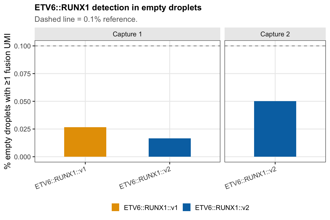
ETV6::RUNX1 transcripts are detected in fewer than 0.1% of empty droplets across both captures, confirming that ambient fusion levels are very low.
Top ambient genes in empty droplets
For context, the same detection rate metric applied to the top 10 most abundant ambient genes (by concentration in the empty-droplet profile), shown alongside the fusion probes.
cap_dirs <- list(
  "Capture 1" = list(
    raw     = here("data", "CAPTURE-1-POOL-FLEX",
                   "outs", "multi", "count", "raw_feature_bc_matrix"),
    samples = here("data", "CAPTURE-1-POOL-FLEX", "outs", "per_sample_outs")
  ),
  "Capture 2" = list(
    raw     = here("data", "Run_1_and_Run_2",
                   "Cellranger_Config_Sample_CAPTURE-2-POOL-FLEX",
                   "outs", "multi", "count", "raw_feature_bc_matrix"),
    samples = here("data", "Run_1_and_Run_2",
                   "Cellranger_Config_Sample_CAPTURE-2-POOL-FLEX",
                   "outs", "per_sample_outs")
  )
)

get_gene_ambient_detection <- function(raw_dir, per_sample_dir, genes, label) {
  filtered_bc       <- get_filtered_barcodes(per_sample_dir)
  raw_sce           <- read10xCounts(raw_dir, col.names = TRUE)
  is_cell           <- colnames(raw_sce) %in% filtered_bc
  symbol_map        <- setNames(rowData(raw_sce)$Symbol, rownames(raw_sce))
  rownames(raw_sce) <- ifelse(is.na(symbol_map[rownames(raw_sce)]),
                              rownames(raw_sce), symbol_map[rownames(raw_sce)])
  rownames(raw_sce) <- gsub("_", "-", rownames(raw_sce))

  keep  <- intersect(genes, rownames(raw_sce))
  ecmat <- counts(raw_sce)[keep, which(!is_cell), drop = FALSE]
  rm(raw_sce); gc()

  data.frame(gene         = keep,
             n_empty      = ncol(ecmat),
             pct_detected = rowMeans(ecmat > 0) * 100,
             capture      = label)
}

get_top_ambient_genes <- function(profile, n = 50) {
  non_fusion <- profile[!grepl("-fusion$", names(profile)) &
                          !grepl("^DEPRECATED_", names(profile))]
  names(sort(non_fusion, decreasing = TRUE))[seq_len(n)]
}

amb_profiles <- list("Capture 1" = amb_cap1, "Capture 2" = amb_cap2)
n_top <- 10

ambient_gene_df <- lapply(names(cap_dirs), function(cap) {
  top_genes <- get_top_ambient_genes(amb_profiles[[cap]], n = n_top)
  get_gene_ambient_detection(cap_dirs[[cap]]$raw,
                             cap_dirs[[cap]]$samples,
                             top_genes, cap)
}) %>% bind_rows()

cat("Top ambient gene detection rates (%):\n")
Top ambient gene detection rates (%):print(ambient_gene_df %>% arrange(capture, desc(pct_detected))) gene n_empty pct_detected capture
CD74...1 CD74 1294116 2.3048166 Capture 1
MT-CO1...2 MT-CO1 1294116 1.4467018 Capture 1
MT-CO3...3 MT-CO3 1294116 1.2009743 Capture 1
TMSB4X...4 TMSB4X 1294116 1.1840515 Capture 1
MT-ATP6...5 MT-ATP6 1294116 1.1506696 Capture 1
MME...6 MME 1294116 1.1067014 Capture 1
LAPTM5...7 LAPTM5 1294116 1.1019878 Capture 1
MT-CO2...8 MT-CO2 1294116 1.0028467 Capture 1
MT-ND3 MT-ND3 1294116 1.0019195 Capture 1
B2M...10 B2M 1294116 0.9883194 Capture 1
CD74...11 CD74 2144325 3.1615543 Capture 2
MT-CO1...12 MT-CO1 2144325 1.7978152 Capture 2
TMSB4X...13 TMSB4X 2144325 1.7016544 Capture 2
CXCR4 CXCR4 2144325 1.6341739 Capture 2
MME...15 MME 2144325 1.5821296 Capture 2
MT-ATP6...16 MT-ATP6 2144325 1.4295874 Capture 2
LAPTM5...17 LAPTM5 2144325 1.3256852 Capture 2
B2M...18 B2M 2144325 1.3244261 Capture 2
MT-CO3...19 MT-CO3 2144325 1.2432817 Capture 2
MT-CO2...20 MT-CO2 2144325 1.1645623 Capture 2# Rank fusion probes among ALL genes by ambient concentration (proxy for
# % droplet detection rate — concentration and detection rate are monotonically
# related so rank order is equivalent)
cat("\n── Observed vs expected non-blast fusion detections ──\n")
── Observed vs expected non-blast fusion detections ──cat(" expected = ambient detection rate (empty droplets) × n non-blast cells\n\n") expected = ambient detection rate (empty droplets) × n non-blast cellscap_vals <- sort(unique(nonblast_exp2$Capture))
ambient_vs_obs <- lapply(cap_vals, function(cap) {
cap_label <- if (cap == cap_vals[1]) "Capture 1" else "Capture 2"
cap_cells <- colnames(nonblast_exp2)[nonblast_exp2$Capture == cap]
n_nb <- length(cap_cells)
probes <- if (cap_label == "Capture 1") patient_fusions else
patient_fusions[grepl("v2", patient_fusions)]
lapply(probes, function(fn) {
n_obs <- sum(counts_mat[fn, cap_cells] > 0)
amb_row <- empty_df[empty_df$fusion == fn & empty_df$capture == cap_label, ]
if (nrow(amb_row) == 0) return(NULL)
n_exp <- (amb_row$pct_detected / 100) * n_nb
data.frame(capture = cap_label,
fusion = clean_label(fn),
n_nonblast = n_nb,
n_observed = n_obs,
n_expected = round(n_exp, 2),
fold_enrichment = round(n_obs / n_exp, 1))
}) %>% bind_rows()
}) %>% bind_rows()
ambient_vs_obs <- ambient_vs_obs %>%
mutate(
p_value = mapply(function(obs, exp) poisson.test(obs, T = 1, r = exp)$p.value,
n_observed, n_expected),
p_adj = p.adjust(p_value, method = "BH")
)
print(ambient_vs_obs) capture fusion n_nonblast n_observed n_expected fold_enrichment
1 Capture 1 ETV6::RUNX1::v1 3266 13 0.87 14.9
2 Capture 1 ETV6::RUNX1::v2 3266 11 0.55 20.2
3 Capture 2 ETV6::RUNX1::v2 4876 65 2.44 26.6
p_value p_adj
1 1.173200e-11 1.759800e-11
2 2.109947e-11 2.109947e-11
3 1.662189e-67 4.986567e-67cat("\n── Fusion probe ranks among all genes (by ambient concentration) ──\n")
── Fusion probe ranks among all genes (by ambient concentration) ──pval_label <- function(p) {
case_when(p < 0.001 ~ "***", p < 0.01 ~ "**", p < 0.05 ~ "*", TRUE ~ "ns")
}
plot_df <- ambient_vs_obs %>%
mutate(label = paste0(capture, "\n", fusion),
sig_label = pval_label(p_adj),
annot = paste0(sig_label, "\n(", fold_enrichment, "×)"))
long_df <- plot_df %>%
select(label, annot, n_observed, n_expected) %>%
pivot_longer(c(n_observed, n_expected),
names_to = "type", values_to = "count") %>%
mutate(type = recode(type,
n_observed = "Observed",
n_expected = "Expected (ambient)"),
type = factor(type, levels = c("Expected (ambient)", "Observed")))
y_floor <- 0.3
p_ambient_poisson <- ggplot(long_df,
aes(x = label, colour = type, shape = type, group = type)) +
geom_linerange(aes(ymin = y_floor, ymax = count),
position = position_dodge(width = 0.4), linewidth = 0.8) +
geom_point(aes(y = count), size = 4,
position = position_dodge(width = 0.4)) +
geom_text(data = plot_df,
aes(x = label, y = n_observed * 2, label = annot),
inherit.aes = FALSE, size = 3.5, lineheight = 0.9) +
scale_y_log10(labels = label_number(accuracy = 1)) +
scale_colour_manual(values = c("Expected (ambient)" = "grey40",
"Observed" = "#D62728"), name = NULL) +
scale_shape_manual(values = c("Expected (ambient)" = 16,
"Observed" = 16), name = NULL) +
labs(x = NULL, y = "Cells with ≥1 fusion UMI (log scale)") +
theme_pub() +
theme(legend.position = "bottom")
p_ambient_poisson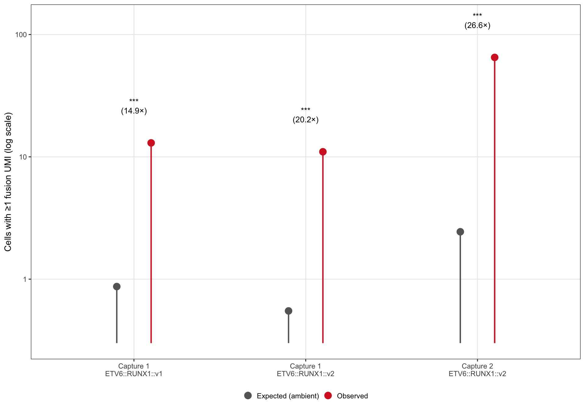
for (cap in names(amb_profiles)) {
  prof <- amb_profiles[[cap]]
  prof <- sort(prof[!grepl("^DEPRECATED_", names(prof))], decreasing = TRUE)
  n_total <- length(prof)
  for (fn in patient_fusions) {
    if (fn %in% names(prof)) {
      rk <- which(names(prof) == fn)
      cat(sprintf("  %s  %s: rank %d of %d (conc = %s)\n",
                  cap, clean_label(fn), rk, n_total,
                  signif(prof[fn], 3)))
    }
  }
}
Capture 1 ETV6::RUNX1::v1: rank 3518 of 37145 (conc = 8.14e-05)
Capture 1 ETV6::RUNX1::v2: rank 7728 of 37145 (conc = 2.7e-05)
Capture 2 ETV6::RUNX1::v1: rank 15248 of 37145 (conc = 1.35e-07)
Capture 2 ETV6::RUNX1::v2: rank 2092 of 37145 (conc = 0.000121)fusion_for_compare <- empty_df %>%
mutate(gene = clean_label(fusion)) %>%
filter(!(gene == "ETV6::RUNX1::v1" & capture == "Capture 2")) %>%
transmute(gene, capture, pct_detected, type = "Fusion probe")
gene_for_compare <- ambient_gene_df %>%
transmute(gene, capture, pct_detected, type = "Ambient gene")
# Order: ambient genes alphabetically, then fusion probes
# Sort ambient genes by mean detection rate across captures (descending)
gene_order_ambient <- gene_for_compare %>%
group_by(gene) %>%
summarise(mean_pct = mean(pct_detected), .groups = "drop") %>%
arrange(desc(mean_pct)) %>%
pull(gene)
gene_order <- c(gene_order_ambient, sort(unique(fusion_for_compare$gene)))
compare_df <- bind_rows(gene_for_compare, fusion_for_compare) %>%
mutate(gene = factor(gene, levels = gene_order),
type = factor(type, levels = c("Ambient gene", "Fusion probe")))
y_min <- min(compare_df$pct_detected) * 0.3
p_ambient_genes <- ggplot(compare_df,
aes(x = gene, y = pct_detected, colour = type)) +
geom_segment(aes(xend = gene, yend = y_min), linewidth = 0.7) +
geom_point(size = 3) +
scale_y_log10(labels = label_number(accuracy = 0.001)) +
scale_colour_manual(values = c("Ambient gene" = "grey50",
"Fusion probe" = "#D62728"),
name = NULL) +
facet_wrap(~ capture, ncol = 2, scales = "free_x") +
labs(
x = NULL,
y = "% empty droplets with ≥1 UMI (log scale)",
title = "Ambient gene vs fusion probe detection in empty droplets"
) +
theme_pub() +
theme(axis.text.x = element_text(angle = 35, hjust = 1),
legend.position = "bottom")
p_ambient_genes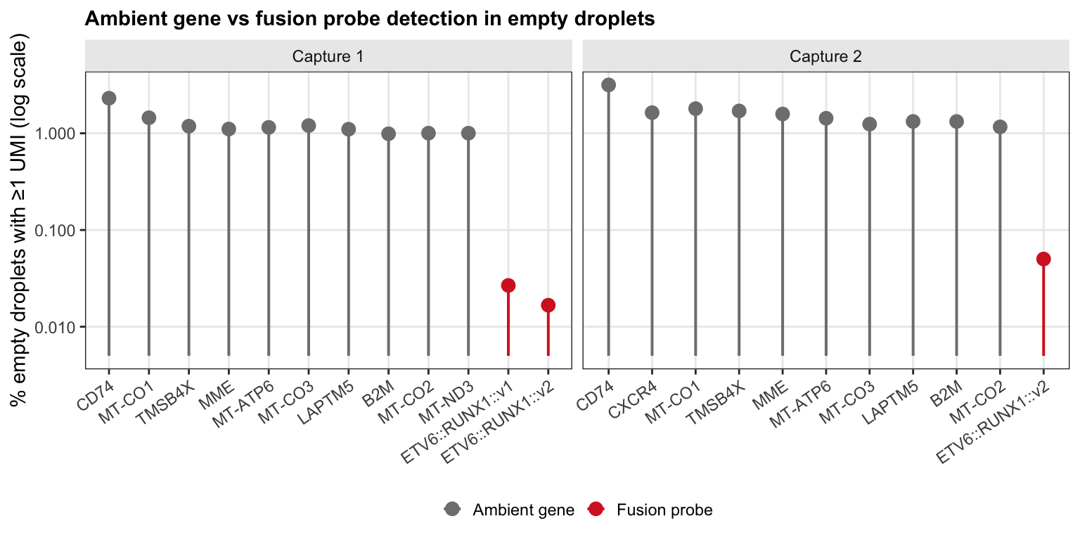
lineage_map <- c(
  "B"                    = "B",
  "Plasma Cell"          = "B",
  "Naive T"              = "T / NK",
  "CD4 Memory T"         = "T / NK",
  "CD8 Memory T"         = "T / NK",
  "NK"                   = "T / NK",
  "Monocyte"             = "Myeloid",
  "pDC"                  = "Myeloid",
  "Late Erythroid"       = "Erythroid",
  "Early Erythroid"      = "Erythroid",
  "Erythroid Progenitor" = "Erythroid"
)

umap_coords <- Embeddings(seu_exp2, "umap") %>%
  as.data.frame() %>%
  setNames(c("UMAP_1", "UMAP_2")) %>%
  rownames_to_column("barcode")

umap_df <- seu_exp2@meta.data %>%
  rownames_to_column("barcode") %>%
  select(barcode, is_blast, cluster_celltype, sample = patient_timepoint) %>%
  left_join(umap_coords, by = "barcode") %>%
  mutate(
    fusion_pos = barcode %in% fusion_pos_barcodes,
    lineage    = lineage_map[cluster_celltype]
  )
Diagnostic: Pro-B cell identity
The blast marker dot plot (Fig 5F) shows some residual signal in the non-blast fusion+ group. Pro-B cells are the most likely source because they are the normal counterpart of B-ALL blasts and share surface markers. This section asks whether fusion+ non-blast Pro-B cells represent boundary annotation cases (cells the cluster-level blast call missed) or genuine normal progenitors.
Two lines of evidence:
- BoneMarrowMap per-cell prediction scores — low max-score or high blast-type score on a Pro-B-labelled cell suggests it sits at the blast/normal boundary and may have been captured in the wrong cluster.
- UMAP position — Pro-B fusion+ cells that fall inside the blast cloud are likely misclassified; those in the distinct Pro-B region are more plausibly normal progenitors carrying the fusion as a molecular scar.
# Step 1 — discover what BoneMarrowMap annotation columns are in the object
score_cols <- grep("score|predict|celltype|label|mapping",
                   colnames(seu_exp2@meta.data),
                   ignore.case = TRUE, value = TRUE)
cat("Available annotation / prediction columns:\n")
Available annotation / prediction columns:cat(paste0(" • ", score_cols, "\n")) • final_labelling
• scDblFinder.score
• scDblFinder.cxds_score
• mapping_error_score
• mapping_error_QC
• initial_CellType_prob
• initial_CellType
• predicted_CellType
• predicted_CellType_prob
• predicted_CellType_Broad
• predicted_CellType_No_Abbreviations
• predicted_Pseudotime
• S.Score
• G2M.Score
• celltype_label
• cluster_celltype# Step 2 — isolate the fusion+ non-blast Pro-B cells
prob_fusion_barcodes <- nonblast_exp2@meta.data %>%
rownames_to_column("barcode") %>%
filter(barcode %in% fusion_pos_barcodes,
cluster_celltype == "Pro-B") %>%
pull(barcode)
cat(glue("Fusion+ non-blast Pro-B cells: {length(prob_fusion_barcodes)}\n"))Fusion+ non-blast Pro-B cells: 0cat("\nBreakdown by patient / timepoint:\n")
Breakdown by patient / timepoint:print(table(seu_exp2@meta.data[prob_fusion_barcodes, "patient_timepoint"]))
C1437_Diagnosis   C1437_Relapse  C369_Diagnosis        C369_MRD    C369_Relapse
              0               0               0               0               0
 C601_Diagnosis  C658_Diagnosis  C659_Diagnosis
              0               0               0
# Step 3 — summarise per-cell BoneMarrowMap prediction scores for these cells
# Seurat MapQuery typically writes prediction.score.max and per-type columns.
# BoneMarrowMap may also write mapping.score or score.* — adapt as needed.
prob_meta <- seu_exp2@meta.data[prob_fusion_barcodes, , drop = FALSE]
# --- max prediction score (overall annotation confidence) ---
max_score_col <- intersect(
c("prediction.score.max", "mapping.score", "score.max"),
colnames(prob_meta)
)
if (length(max_score_col) > 0) {
col <- max_score_col[1]
cat(glue("\nMax prediction score ({col}) — fusion+ non-blast Pro-B cells:\n"))
print(summary(prob_meta[[col]]))
# Compare with blast cells (positive control — should have high confidence)
blast_meta <- seu_exp2@meta.data[blast_fusion_cells, , drop = FALSE]
if (col %in% colnames(blast_meta)) {
cat(glue("\nMax prediction score ({col}) — fusion+ blast cells (positive control):\n"))
print(summary(blast_meta[[col]]))
}
} else {
cat("No max-score column found. Check score_cols above and adjust.\n")
}No max-score column found. Check score_cols above and adjust.# --- per-cell-type scores: look for any blast-related type score ---
blast_type_cols <- grep("blast|B_ALL|leuk",
colnames(prob_meta), ignore.case = TRUE, value = TRUE)
if (length(blast_type_cols) > 0) {
cat("\nBlast-type score columns found:", paste(blast_type_cols, collapse = ", "), "\n")
cat("\nSummary for fusion+ non-blast Pro-B cells:\n")
print(summary(prob_meta[, blast_type_cols, drop = FALSE]))
} else {
cat("\nNo explicit blast-type score column found in metadata.\n")
cat("All per-cell-type score columns present:\n")
all_per_type <- grep("^prediction\\.score\\.", colnames(prob_meta), value = TRUE)
if (length(all_per_type) > 0) {
print(summary(prob_meta[, all_per_type, drop = FALSE]))
} else {
cat(" (none — scores may be stored differently; see score_cols above)\n")
}
}
Blast-type score columns found: percent_blasts_in_bone_marrow, is_blast

Summary for fusion+ non-blast Pro-B cells:
 percent_blasts_in_bone_marrow is_blast
 Min.   : NA                   Mode:logical
 1st Qu.: NA
 Median : NA
 Mean   :NaN
 3rd Qu.: NA
 Max.   : NA
# Step 4 — UMAP highlighting where fusion+ non-blast Pro-B cells sit
# relative to the blast mass and the normal Pro-B region
highlight_levels <- c(
"Blast (fusion−)",
"Blast (fusion+)",
"Non-blast Pro-B (fusion−)",
"Non-blast Pro-B (fusion+)",
"Other non-blast"
)
umap_prob_df <- umap_df %>%
mutate(
highlight = case_when(
is_blast & barcode %in% blast_fusion_cells ~ "Blast (fusion+)",
is_blast ~ "Blast (fusion−)",
!is_blast & barcode %in% prob_fusion_barcodes ~ "Non-blast Pro-B (fusion+)",
!is_blast & cluster_celltype == "Pro-B" ~ "Non-blast Pro-B (fusion−)",
TRUE ~ "Other non-blast"
),
highlight = factor(highlight, levels = highlight_levels)
) %>%
# Plot order: blasts first, then non-blast, then highlighted cells on top
arrange(highlight)
highlight_pal <- c(
"Blast (fusion−)" = "grey75",
"Blast (fusion+)" = "#CB181D",
"Non-blast Pro-B (fusion−)" = "#9ECAE1",
"Non-blast Pro-B (fusion+)" = "#08519C",
"Other non-blast" = "grey92"
)
p_umap_prob <- ggplot(umap_prob_df,
aes(UMAP_1, UMAP_2, colour = highlight,
size = highlight, alpha = highlight)) +
geom_point() +
scale_colour_manual(values = highlight_pal, name = NULL) +
scale_size_manual(
values = c(
"Blast (fusion−)" = 0.12,
"Blast (fusion+)" = 0.8,
"Non-blast Pro-B (fusion−)" = 0.12,
"Non-blast Pro-B (fusion+)" = 2.5,
"Other non-blast" = 0.12
), name = NULL
) +
scale_alpha_manual(
values = c(
"Blast (fusion−)" = 0.3,
"Blast (fusion+)" = 0.9,
"Non-blast Pro-B (fusion−)" = 0.5,
"Non-blast Pro-B (fusion+)" = 1.0,
"Other non-blast" = 0.5
), name = NULL
) +
labs(
x = "UMAP 1",
y = "UMAP 2",
title = "Diagnostic: fusion+ non-blast Pro-B cells in UMAP space",
subtitle = "Large dark-blue dots = fusion+ Pro-B cells classified as non-blast"
) +
theme_classic(base_size = 10) +
theme(
axis.text = element_blank(),
axis.ticks = element_blank(),
axis.line = element_blank(),
legend.text = element_text(size = 8),
plot.title = element_text(face = "bold", size = 11),
plot.subtitle = element_text(size = 9, colour = "grey40")
) +
guides(colour = guide_legend(override.aes = list(size = 3, alpha = 1)))
p_umap_prob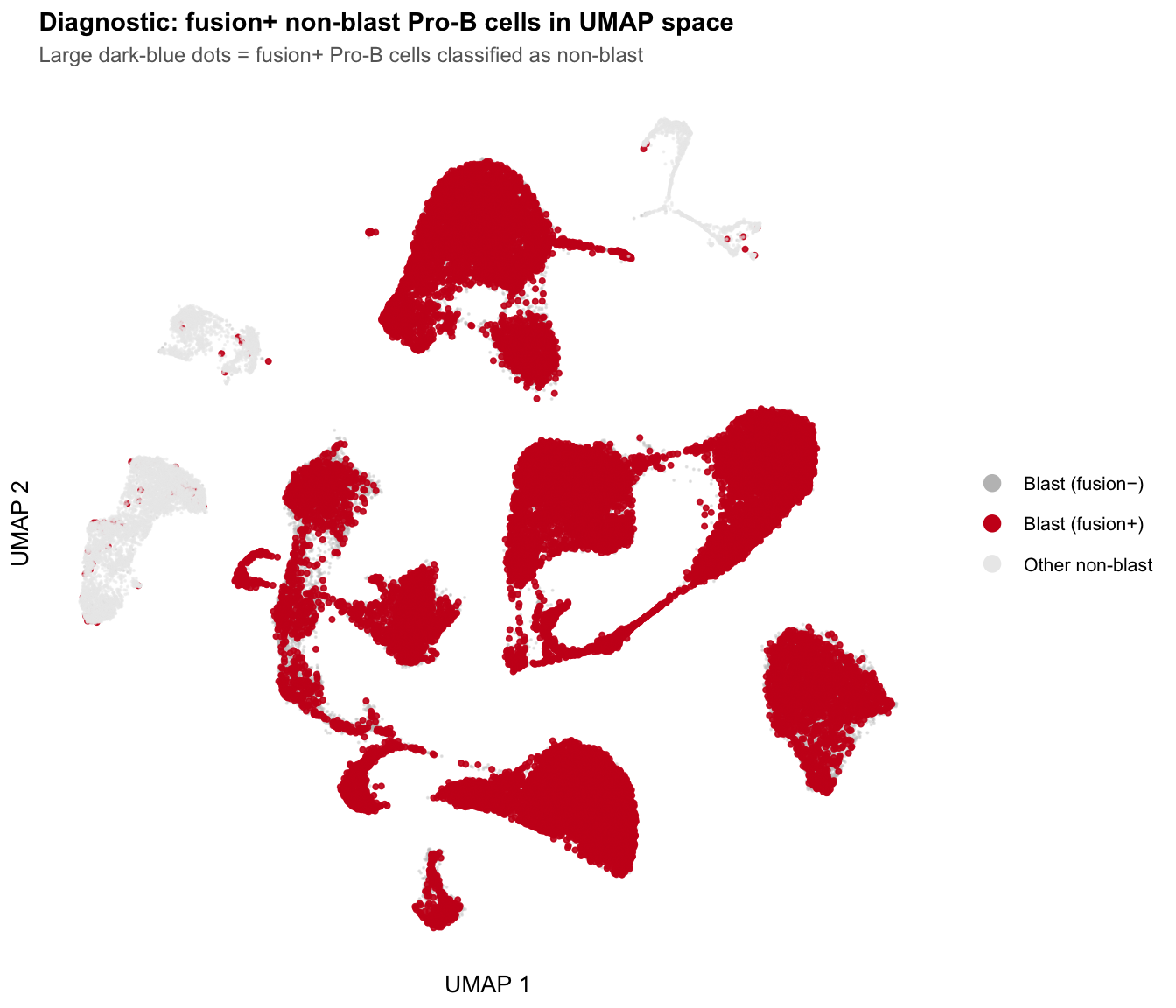
Joint UMAP
All Exp2 cells plotted on the joint UMAP. Blast cells are coloured by patient/timepoint. Non-blast fusion-negative cells are shown in light grey. Non-blast fusion-positive cells are plotted as larger, fully opaque points coloured by patient/timepoint, making both their lineage position and patient of origin immediately visible. The key observation is that fusion-positive non-blast cells sit within their respective normal haematopoietic compartments rather than clustering with the blast mass.
# Corner UMAP arrow annotation (bottom-left) — matches joint clustering notebook
umap_arrow <- annotation_custom(
  grob = grid::grobTree(
    grid::segmentsGrob(
      x0 = 0.05, y0 = 0.05, x1 = 0.16, y1 = 0.05,
      arrow = grid::arrow(length = grid::unit(0.15, "cm"), type = "closed"),
      gp = grid::gpar(fill = "grey20", col = "grey20", lwd = 2.5)
    ),
    grid::segmentsGrob(
      x0 = 0.05, y0 = 0.05, x1 = 0.05, y1 = 0.16,
      arrow = grid::arrow(length = grid::unit(0.15, "cm"), type = "closed"),
      gp = grid::gpar(fill = "grey20", col = "grey20", lwd = 2.5)
    ),
    grid::textGrob("UMAP", x = 0.105, y = 0.01,
      gp = grid::gpar(fontsize = 8, col = "grey20", fontface = "bold"))
  )
)

# Lineage centroids for broad labels (from non-blast fusion- cells only)
centroids <- umap_df %>%
  filter(!is_blast, !fusion_pos, !is.na(lineage)) %>%
  group_by(lineage) %>%
  summarise(UMAP_1 = median(UMAP_1), UMAP_2 = median(UMAP_2), .groups = "drop")

p_umap <- ggplot() +
  # Blast cells — coloured by patient / timepoint
  geom_point(data    = filter(umap_df, is_blast),
             mapping = aes(UMAP_1, UMAP_2, colour = sample),
             size = 0.15, alpha = 0.4) +
  # Non-blast fusion- — warm mid-grey (distinct from C369_MRD lavender)
  geom_point(data    = filter(umap_df, !is_blast, !fusion_pos),
             mapping = aes(UMAP_1, UMAP_2),
             colour  = "#D8D8D8", size = 0.25, alpha = 0.05) +
  # Non-blast fusion+ — same patient palette, larger, fully opaque
  geom_point(data    = filter(umap_df, !is_blast, fusion_pos),
             mapping = aes(UMAP_1, UMAP_2, colour = sample),
             size = 1.8, alpha = 1) +
  # Lineage labels at cluster centroids
  geom_text_repel(
    data           = centroids,
    mapping        = aes(UMAP_1, UMAP_2, label = lineage),
    size           = 3, colour = "grey20", fontface = "bold",
    box.padding    = 0.3, point.padding = 0.1,
    segment.colour = "grey50", segment.size  = 0.3,
    max.overlaps   = 20
  ) +
  scale_colour_manual(values   = sample_palette,
                      na.value = "#D8D8D8",
                      name     = "Patient / timepoint") +
  labs(x = NULL, y = NULL) +
  coord_cartesian(clip = "off") +
  theme_classic(base_size = 10) +
  theme(
    axis.text    = element_blank(),
    axis.ticks   = element_blank(),
    axis.line    = element_blank(),
    legend.text  = element_text(size = 8),
    legend.title = element_text(size = 8, face = "bold")
  ) +
  umap_arrow +
  guides(colour = guide_legend(override.aes = list(size = 3, alpha = 1), ncol = 1))

p_umap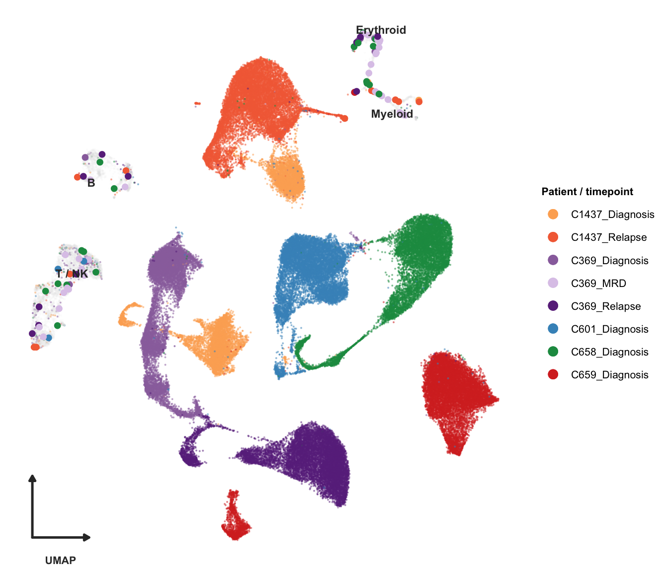
Cell type composition
Which non-blast cell types carry ETV6::RUNX1 fusion transcripts, and does the pattern of detections span multiple lineages consistent with a multipotent progenitor origin?
meta_nonblast <- nonblast_exp2@meta.data %>%
  rownames_to_column("barcode") %>%
  mutate(
    fusion_pos = barcode %in% fusion_pos_barcodes,
    ct = ifelse(cluster_celltype %in% ct_order[ct_order != "Other"],
                cluster_celltype, "Other"),
    ct = factor(ct, levels = rev(ct_order))
  )

counts_ct <- meta_nonblast %>%
  filter(fusion_pos) %>%
  count(ct, .drop = FALSE) %>%
  filter(n > 0)

pct_ct <- meta_nonblast %>%
  group_by(ct) %>%
  summarise(pct = mean(fusion_pos) * 100, .groups = "drop") %>%
  filter(pct > 0)
ct_combined <- counts_ct %>%
left_join(pct_ct, by = "ct") %>%
mutate(bar_label = paste0(n, " (", number(pct, accuracy = 0.01), "%)"))
p_celltype <- ggplot(ct_combined, aes(x = n, y = ct)) +
geom_col(width = 0.7, fill = "grey60", show.legend = FALSE) +
geom_text(aes(label = bar_label), hjust = -0.1, size = 3) +
scale_x_continuous(expand = expansion(mult = c(0, 0.4))) +
labs(x = "Fusion+ non-blast cells (n)", y = NULL) +
theme_pub(base_size = 10)
p_celltype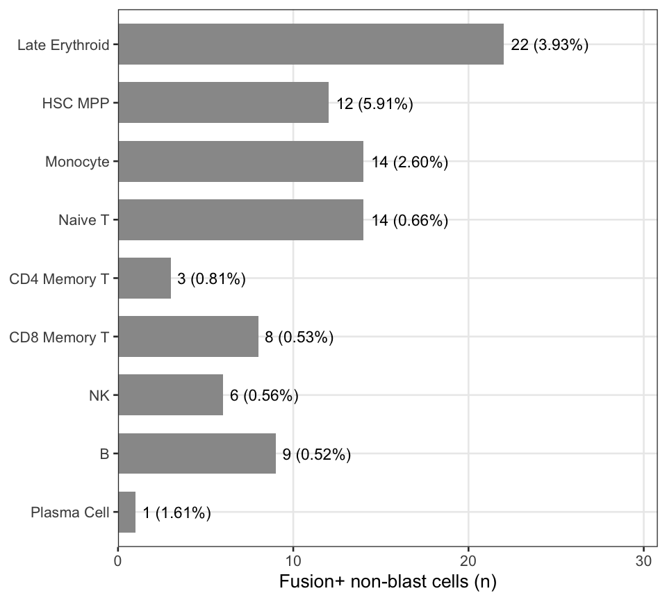
Fusion UMI distributions
Per-cell fusion UMI counts in non-blast cells on a log scale, coloured by cell type. The grey crossbar marks the ambient expectation: ambient concentration × mean total UMI per non-blast cell, computed per capture. Cells substantially above the ambient bar have more fusion transcripts than expected from ambient contamination alone.
cap_vals <- sort(unique(nonblast_exp2$Capture))

# Ambient concentrations indexed by capture
amb_conc_v1 <- setNames(c(amb_cap1["ETV6-RUNX1-v1-fusion"],
                           amb_cap2["ETV6-RUNX1-v1-fusion"]), cap_vals)
amb_conc_v2 <- setNames(c(amb_cap1["ETV6-RUNX1-v2-fusion"],
                           amb_cap2["ETV6-RUNX1-v2-fusion"]), cap_vals)

mean_umi_per_cap <- nonblast_exp2@meta.data %>%
  group_by(Capture) %>%
  summarise(mean_total = mean(nCount_RNA), .groups = "drop")

# Extract per-probe UMI counts for fusion+ non-blast cells (matrix approach)
v1_counts <- counts_mat["ETV6-RUNX1-v1-fusion", ]
v2_counts <- counts_mat["ETV6-RUNX1-v2-fusion", ]

fusion_umi_df <- nonblast_exp2@meta.data %>%
  rownames_to_column("barcode") %>%
  filter(barcode %in% fusion_pos_barcodes) %>%
  left_join(mean_umi_per_cap, by = "Capture") %>%
  mutate(
    cell_type = cluster_celltype,
    v1_umi    = v1_counts[barcode],
    v2_umi    = v2_counts[barcode]
  ) %>%
  pivot_longer(c(v1_umi, v2_umi),
               names_to = "probe", values_to = "fusion_umi") %>%
  filter(fusion_umi > 0) %>%
  mutate(
    probe_label = if_else(probe == "v1_umi", "ETV6::RUNX1-v1", "ETV6::RUNX1-v2"),
    amb_exp     = if_else(probe == "v1_umi",
                          amb_conc_v1[Capture], amb_conc_v2[Capture]) * mean_total
  ) %>%
  # v1 probe only present in Capture 1
  filter(!(probe == "v1_umi" & Capture == cap_vals[2]))

# Ambient reference lines per capture × probe
amb_line_df <- bind_rows(
  data.frame(Capture     = cap_vals[1],
             probe_label = "ETV6::RUNX1-v1",
             amb_y = amb_conc_v1[cap_vals[1]] *
               mean_umi_per_cap$mean_total[mean_umi_per_cap$Capture == cap_vals[1]]),
  mean_umi_per_cap %>%
    mutate(probe_label = "ETV6::RUNX1-v2",
           amb_y = amb_conc_v2[Capture] * mean_total)
)

p_umi <- ggplot(fusion_umi_df,
       aes(x = probe_label, y = fusion_umi, colour = cell_type)) +
  geom_crossbar(data        = amb_line_df,
                aes(x = probe_label, y = amb_y, ymin = amb_y, ymax = amb_y),
                width = 0.5, colour = "grey40", linewidth = 0.5,
                inherit.aes = FALSE) +
  geom_jitter(width = 0.15, size = 2, alpha = 0.8) +
  scale_y_log10(labels = label_comma()) +
  scale_colour_manual(values = ct_palette, name = "Cell type",
                      na.value = "grey70") +
  facet_wrap(~ Capture, scales = "free_x") +
  labs(
    x        = NULL,
    y        = "Fusion UMI per cell (log scale)",
    subtitle = "Grey bar = ambient expectation (concentration × mean total UMI)"
  ) +
  theme_pub() +
  theme(axis.text.x = element_text(angle = 20, hjust = 1))

p_umi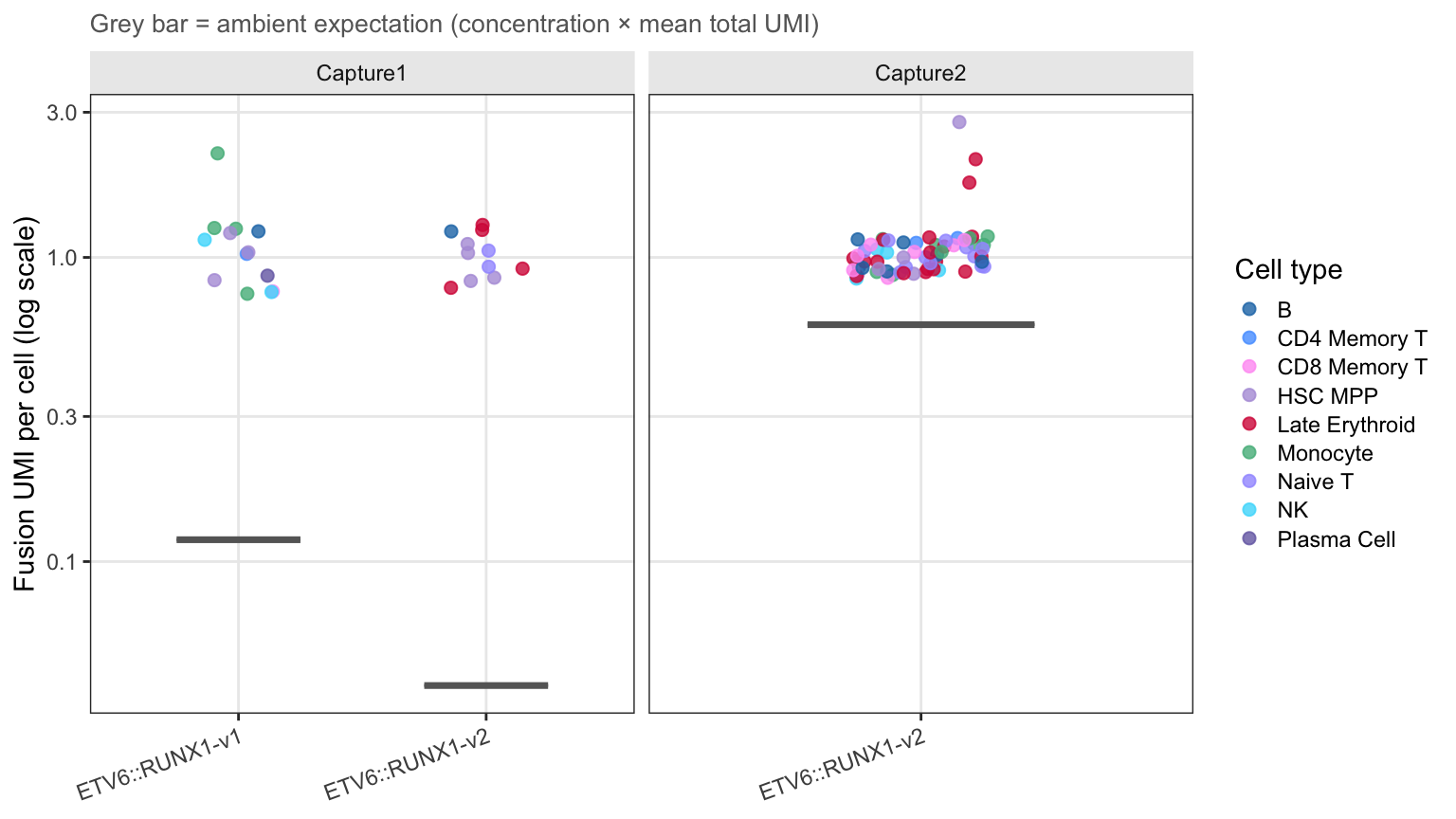
Patient and timepoint enrichment
Non-blast ETV6::RUNX1 detections across all patients and timepoints, shown as the percentage of non-blast cells that are fusion-positive. Tile fill = rate; label = absolute cell count (blank where zero).
sample_totals <- nonblast_exp2@meta.data %>%
  count(patient_timepoint, name = "n_nonblast")

# Per-barcode probe assignment (a cell may be v1+, v2+, or both)
v1_barcodes <- fusion_pos_barcodes[v1_counts[fusion_pos_barcodes] > 0]
v2_barcodes <- fusion_pos_barcodes[v2_counts[fusion_pos_barcodes] > 0]

sample_meta <- nonblast_exp2@meta.data %>%
  rownames_to_column("barcode") %>%
  select(barcode, patient_timepoint)

fusion_long <- bind_rows(
  data.frame(barcode = v1_barcodes, fusion_label = "ETV6::RUNX1-v1"),
  data.frame(barcode = v2_barcodes, fusion_label = "ETV6::RUNX1-v2")
) %>%
  left_join(sample_meta, by = "barcode") %>%
  count(patient_timepoint, fusion_label, name = "n_pos")

sample_order <- c(
  "C1437_Diagnosis", "C1437_Relapse", "C659_Diagnosis", "C369_Diagnosis",
  "C369_MRD",        "C369_Relapse",  "C658_Diagnosis", "C601_Diagnosis"
)

heatmap_df <- tidyr::expand_grid(
  patient_timepoint = unique(sample_totals$patient_timepoint),
  fusion_label      = c("ETV6::RUNX1-v1", "ETV6::RUNX1-v2")
) %>%
  left_join(sample_totals,  by = "patient_timepoint") %>%
  left_join(fusion_long,    by = c("patient_timepoint", "fusion_label")) %>%
  mutate(
    n_pos        = replace_na(n_pos, 0L),
    rate         = n_pos / n_nonblast * 100,
    sample_label = factor(gsub("_", " ", patient_timepoint),
                          levels = gsub("_", " ", sample_order))
  )
cap1_samples <- c("C1437_Diagnosis", "C1437_Relapse", "C369_Diagnosis", "C659_Diagnosis")
cap2_samples <- c("C369_Relapse", "C369_MRD", "C601_Diagnosis", "C658_Diagnosis")
patient_counts <- nonblast_exp2@meta.data %>%
rownames_to_column("barcode") %>%
filter(barcode %in% fusion_pos_barcodes) %>%
count(patient_timepoint, name = "n_pos") %>%
right_join(data.frame(patient_timepoint = sample_order), by = "patient_timepoint") %>%
replace_na(list(n_pos = 0L)) %>%
left_join(sample_totals, by = "patient_timepoint") %>%
mutate(
pct = n_pos / n_nonblast * 100,
bar_label = if_else(n_pos == 0L, "0",
paste0(n_pos, " (", sprintf("%.1f%%", pct), ")")),
capture = if_else(patient_timepoint %in% cap1_samples,
"Capture 1", "Capture 2"),
patient_timepoint = factor(patient_timepoint, levels = rev(sample_order))
)
p_patient_bar <- ggplot(patient_counts,
aes(x = n_pos, y = patient_timepoint, fill = patient_timepoint)) +
geom_col(width = 0.7, show.legend = FALSE) +
geom_text(aes(label = bar_label), hjust = -0.1, size = 3) +
scale_fill_manual(values = sample_palette) +
scale_x_continuous(expand = expansion(mult = c(0, 0.3))) +
facet_grid(capture ~ ., scales = "free_y", space = "free_y") +
labs(x = "Fusion+ non-blast cells (n)", y = NULL) +
theme_pub(base_size = 10) +
theme(
strip.background = element_blank(),
strip.text.y = element_text(angle = 90, face = "bold", size = 9,
colour = "grey40")
)
p_patient_bar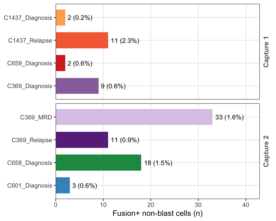
Blast marker expression
If non-blast fusion-positive cells were misclassified blasts or driven by ambient RNA from the blast-rich soup, they would express canonical B-precursor markers (CD19, DNTT, MME, CD34). Genuine pre-leukaemic progenitor progeny that have differentiated normally should not express these markers.
# One canonical marker per lineage group
markers_bm <- c("DNTT", "CD3E", "GNLY", "HBB", "CD14", "CD19", "MZB1")
DefaultAssay(seu_exp2) <- "SCT"

marker_counts_all <- GetAssayData(seu_exp2, assay = "SCT",
                                  layer = "counts")[markers_bm, ]
marker_norm_all   <- GetAssayData(seu_exp2, assay = "SCT",
                                  layer = "data")[markers_bm, ]

compute_dot_df <- function(cells, group_label) {
  lapply(markers_bm, function(gn) {
    cv <- as.numeric(marker_counts_all[gn, cells])
    nv <- as.numeric(marker_norm_all[gn, cells])
    data.frame(
      marker         = gn,
      group          = group_label,
      n              = length(cells),
      pct_expressing = mean(cv > 0) * 100,
      mean_expr      = ifelse(any(cv > 0), mean(nv[cv > 0]), NA_real_)
    )
  }) %>% bind_rows()
}

# Map non-blast fusion+ cells to lineages — T and NK split
nb_lineage_map <- c(
  "B"                    = "B",
  "Plasma Cell"          = "Plasma Cell",
  "Naive T"              = "T",
  "CD4 Memory T"         = "T",
  "CD8 Memory T"         = "T",
  "NK"                   = "NK",
  "Monocyte"             = "Myeloid",
  "pDC"                  = "Myeloid",
  "Late Erythroid"       = "Erythroid",
  "Early Erythroid"      = "Erythroid",
  "Erythroid Progenitor" = "Erythroid"
)

nb_lineage_df <- nonblast_exp2@meta.data %>%
  rownames_to_column("barcode") %>%
  filter(barcode %in% fusion_pos_barcodes) %>%
  mutate(lineage = nb_lineage_map[cluster_celltype],
         lineage = replace_na(lineage, "Other"))

group_levels <- c("ETV6::RUNX1+\nblasts", "T", "NK", "Erythroid", "Myeloid", "B", "Plasma Cell")

dot_df <- bind_rows(
  compute_dot_df(blast_fusion_cells, "ETV6::RUNX1+\nblasts"),
  lapply(c("T", "NK", "Erythroid", "Myeloid", "B", "Plasma Cell"), function(lin) {
    cells <- nb_lineage_df$barcode[nb_lineage_df$lineage == lin]
    if (length(cells) > 0) compute_dot_df(cells, lin)
  }) %>% bind_rows()
) %>%
  mutate(
    marker = factor(marker, levels = rev(markers_bm)),
    group  = factor(group, levels = group_levels)
  )

group_n <- dot_df %>%
  distinct(group, n) %>%
  mutate(label = paste0("n=", comma(n)))

p_markers <- ggplot(dot_df, aes(x = group, y = marker,
                   size = pct_expressing, colour = mean_expr)) +
  geom_point(alpha = 0.9) +
  geom_text(data        = group_n,
            aes(x = group, y = Inf, label = label),
            size = 2.8, colour = "grey30", fontface = "italic",
            vjust = -0.3, inherit.aes = FALSE) +
  geom_vline(xintercept = 1.5, linetype = "dashed",
             colour = "grey60", linewidth = 0.4) +
  scale_colour_distiller(
    palette   = "Purples", direction = 1,
    limits    = c(0, 2.5), oob = scales::squish,
    breaks    = c(0, 1, 2, 2.5), labels = c("0", "1", "2", ">2.5"),
    name      = "Mean\nexpr.", na.value = "grey85",
    guide     = guide_colourbar(direction = "horizontal",
                                title.position = "left",
                                barwidth = 6, barheight = 0.5)
  ) +
  scale_size_continuous(
    name  = "% expr.", range = c(0.5, 8),
    breaks = c(1, 25, 50, 75), limits = c(0, 100),
    guide = guide_legend(direction = "horizontal",
                         title.position = "left", nrow = 1)
  ) +
  labs(x = NULL, y = NULL) +
  theme_classic(base_size = 11) +
  theme(
    axis.text.x      = element_text(size = 9, hjust = 0.5),
    axis.text.y      = element_text(size = 9),
    panel.grid.major = element_line(colour = "grey92", linewidth = 0.3),
    legend.position  = "bottom",
    legend.box       = "horizontal",
    plot.margin      = margin(t = 20, r = 5, b = 5, l = 5)
  ) +
  coord_cartesian(clip = "off")

p_markers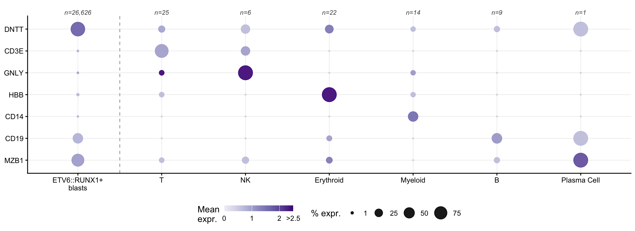
Non-blast fusion-positive cells show no appreciable expression of CD19, DNTT, MME, or CD34 relative to fusion-positive blast cells, confirming they are not misclassified blasts.
Ambient contamination score
If sporadic fusion detections in non-blast cells were driven by ambient contamination, fusion-positive cells should carry more ambient RNA overall. The ambient contamination score is a module score derived from the top 50 genes by ambient concentration in each capture’s empty-droplet profile. Fusion-positive and fusion-negative non-blast cells of the same type are compared by Wilcoxon rank-sum test (BH-adjusted). Cell types with fewer than 3 fusion-positive cells are excluded.
n_ambient_genes <- 50

top_genes_cap1 <- get_top_ambient_genes(amb_cap1, n_ambient_genes)
top_genes_cap2 <- get_top_ambient_genes(amb_cap2, n_ambient_genes)

score_cap_subset <- function(seu, cap_label, top_genes) {
  cells <- colnames(seu)[seu$Capture == cap_label]
  sub   <- seu[, cells]
  sub   <- AddModuleScore(sub, features = list(top_genes), name = "ambient_score")
  setNames(sub$ambient_score1, cells)
}

scores_cap1 <- score_cap_subset(nonblast_exp2, cap_vals[1], top_genes_cap1)
scores_cap2 <- score_cap_subset(nonblast_exp2, cap_vals[2], top_genes_cap2)
combined_scores <- c(scores_cap1, scores_cap2)
nonblast_exp2$ambient_score <- combined_scores[colnames(nonblast_exp2)]
amb_score_df <- nonblast_exp2@meta.data %>%
rownames_to_column("barcode") %>%
select(barcode, ambient_score, cluster_celltype) %>%
mutate(
fusion_pos = barcode %in% fusion_pos_barcodes,
status = if_else(fusion_pos, "Fusion+", "Fusion−")
) %>%
filter(!is.na(ambient_score), !is.na(cluster_celltype))
# Keep cell types with ≥3 fusion+ cells
keep_ct <- amb_score_df %>%
filter(fusion_pos) %>%
count(cluster_celltype) %>%
filter(n >= 3)
amb_score_plot <- amb_score_df %>%
inner_join(keep_ct %>% select(cluster_celltype),
by = "cluster_celltype") %>%
mutate(panel = cluster_celltype)
amb_wilcox <- amb_score_plot %>%
group_by(panel) %>%
summarise(
n_pos = sum(status == "Fusion+"),
n_neg = sum(status == "Fusion−"),
p_value = tryCatch(
wilcox.test(ambient_score[status == "Fusion+"],
ambient_score[status == "Fusion−"],
exact = FALSE)$p.value,
error = function(e) NA_real_
),
.groups = "drop"
) %>%
mutate(
p_adj = p.adjust(p_value, method = "BH"),
sig = case_when(
is.na(p_adj) ~ "",
p_adj < 0.001 ~ "***",
p_adj < 0.01 ~ "**",
p_adj < 0.05 ~ "*",
TRUE ~ "ns"
)
)
cat("Ambient score Wilcoxon results:\n")Ambient score Wilcoxon results:print(amb_wilcox %>% select(panel, n_pos, p_adj, sig) %>% arrange(p_adj))# A tibble: 8 × 4
panel n_pos p_adj sig
<chr> <int> <dbl> <chr>
1 CD4 Memory T 3 0.201 ns
2 HSC MPP 12 0.201 ns
3 CD8 Memory T 8 0.359 ns
4 Late Erythroid 22 0.359 ns
5 B 9 0.887 ns
6 Monocyte 14 0.887 ns
7 NK 6 0.887 ns
8 Naive T 14 0.887 ns y_max_df <- amb_score_plot %>%
group_by(panel) %>%
summarise(y_max = max(ambient_score, na.rm = TRUE) * 1.05, .groups = "drop")
ann_df <- amb_wilcox %>%
left_join(y_max_df, by = "panel") %>%
mutate(ann_label = paste0(sig, "\nn+=", n_pos))
p_ambient <- ggplot(amb_score_plot,
aes(x = status, y = ambient_score, fill = status)) +
geom_violin(scale = "width", linewidth = 0.3, alpha = 0.8) +
geom_boxplot(width = 0.15, fill = "white", outlier.size = 0.5,
linewidth = 0.3, alpha = 0.8) +
geom_text(data = ann_df,
aes(x = 1.5, y = y_max, label = ann_label),
inherit.aes = FALSE, size = 2.2, colour = "grey20",
lineheight = 0.9) +
facet_wrap(~ panel, scales = "free_y", ncol = 4) +
coord_cartesian(clip = "off") +
scale_fill_manual(
values = c("Fusion+" = "#D62728", "Fusion−" = "#AEC7E8"),
name = NULL
) +
labs(
x = NULL,
y = "Ambient contamination score",
subtitle = "Higher score = more ambient RNA. ns / * / ** / *** = BH-adjusted Wilcoxon"
) +
theme_pub() +
theme(legend.position = "bottom",
strip.text = element_text(face = "bold", size = 8))
p_ambient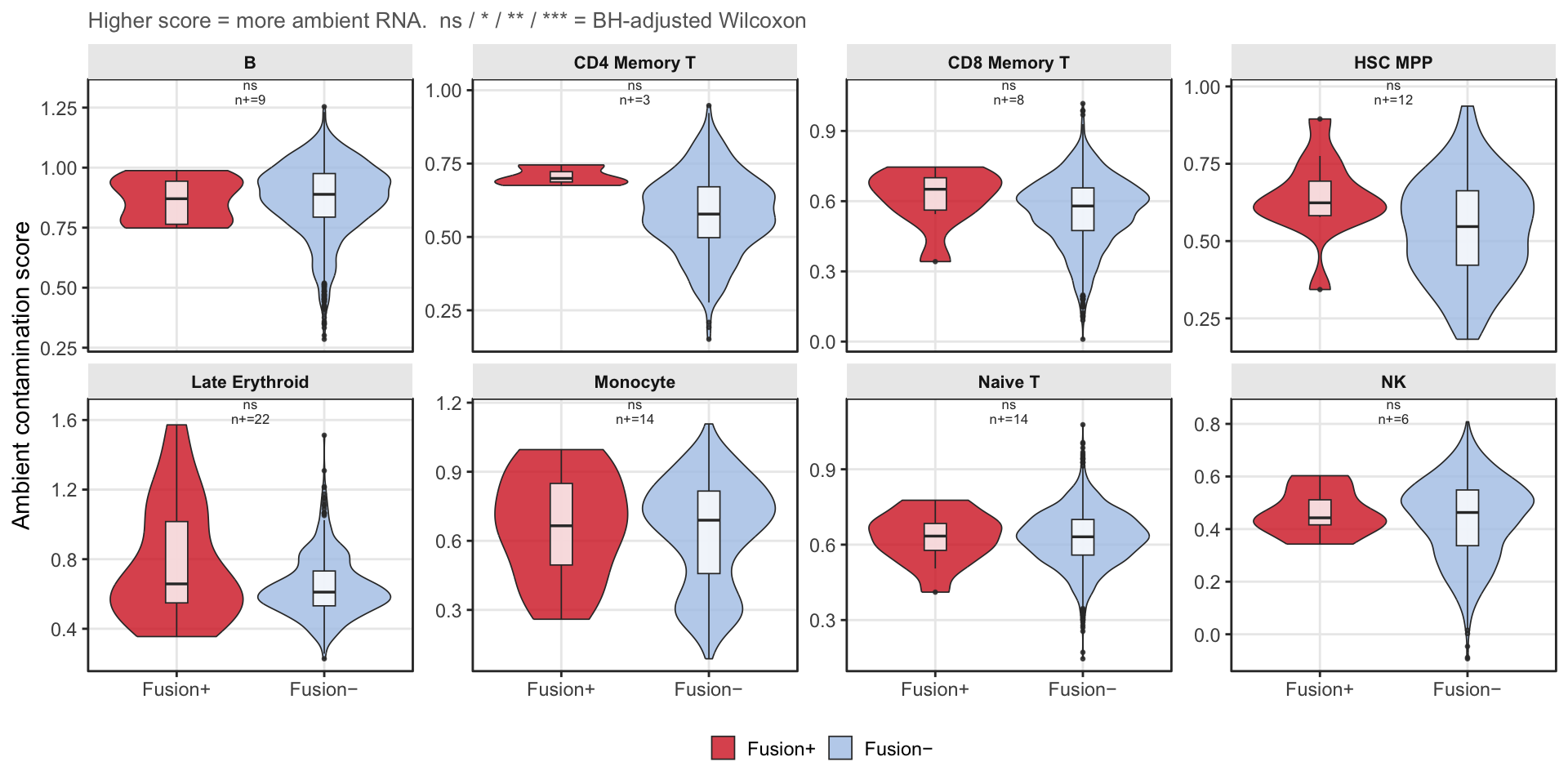
Figure 5
tt <- function(p, title) p + labs(title = title, subtitle = NULL) +
  theme(plot.title = element_text(size = 9, face = "bold", colour = "black",
                                  margin = margin(b = 8)))

tag_theme <- theme(plot.tag = element_text(size = 18, face = "bold"))

pA <- wrap_elements(tt(p_umap,          "ETV6::RUNX1 fusion+ cells localise to non-blast compartments")) + tag_theme
pB <- wrap_elements(tt(p_patient_bar,   "Fusion+ non-blast cells per patient"))   + tag_theme
pC <- wrap_elements(tt(p_celltype,      "Fusion+ non-blast cells by cell type"))  + tag_theme
pD <- wrap_elements(tt(p_markers,       "Non-blast identity confirmed by lineage markers")) + tag_theme
pE <- wrap_elements(tt(p_ambient_poisson, "Fusion detections exceed ambient expectation"))  + tag_theme

fig5 <- (
  pA /
  (pB | pC) /
  (pD | pE)
) +
  plot_layout(heights = c(3.5, 2.2, 2.2)) +
  plot_annotation(tag_levels = "A")

fig5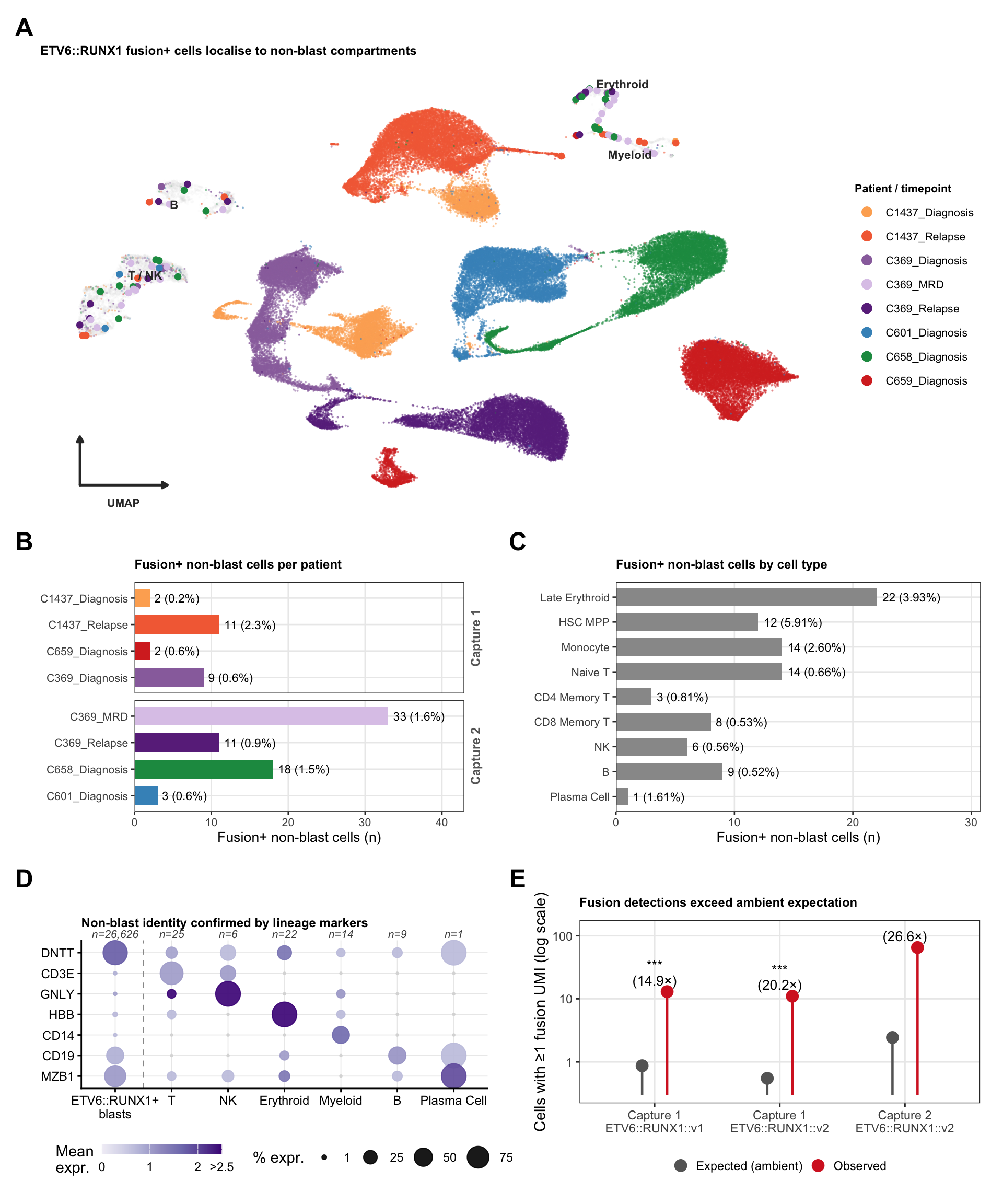
Supplementary Figure 6
Three panels supporting the ambient RNA analysis in Figure 5E. (A) Percentage of empty droplets in which ETV6::RUNX1-v1 (Capture 1 only) and ETV6::RUNX1-v2 fusion transcripts are detected, establishing the ambient null detection rate used in the Poisson test. (B) Detection rate (% empty droplets) for the top 10 ambient genes alongside fusion probes per capture, sorted by decreasing rate. Fusions rank well below the most abundant ambient transcripts, indicating low ambient fusion levels. (C) Ambient RNA score (mean scaled expression of the top 50 ambient genes) in fusion-positive versus fusion-negative non-blast cells, stratified by cell type. Fusion-positive non-blast cells do not show elevated ambient scores relative to fusion-negative cells of the same type.
nt <- function(p) p + labs(title = NULL, subtitle = NULL)

supp_fig <- (
  (nt(p_empty) | nt(p_ambient_genes)) /
  wrap_elements(nt(p_ambient))
) +
  plot_layout(heights = c(1.2, 1.8)) +
  plot_annotation(
    tag_levels = "A",
    theme      = theme(plot.tag = element_text(size = 14, face = "bold"))
  )

supp_fig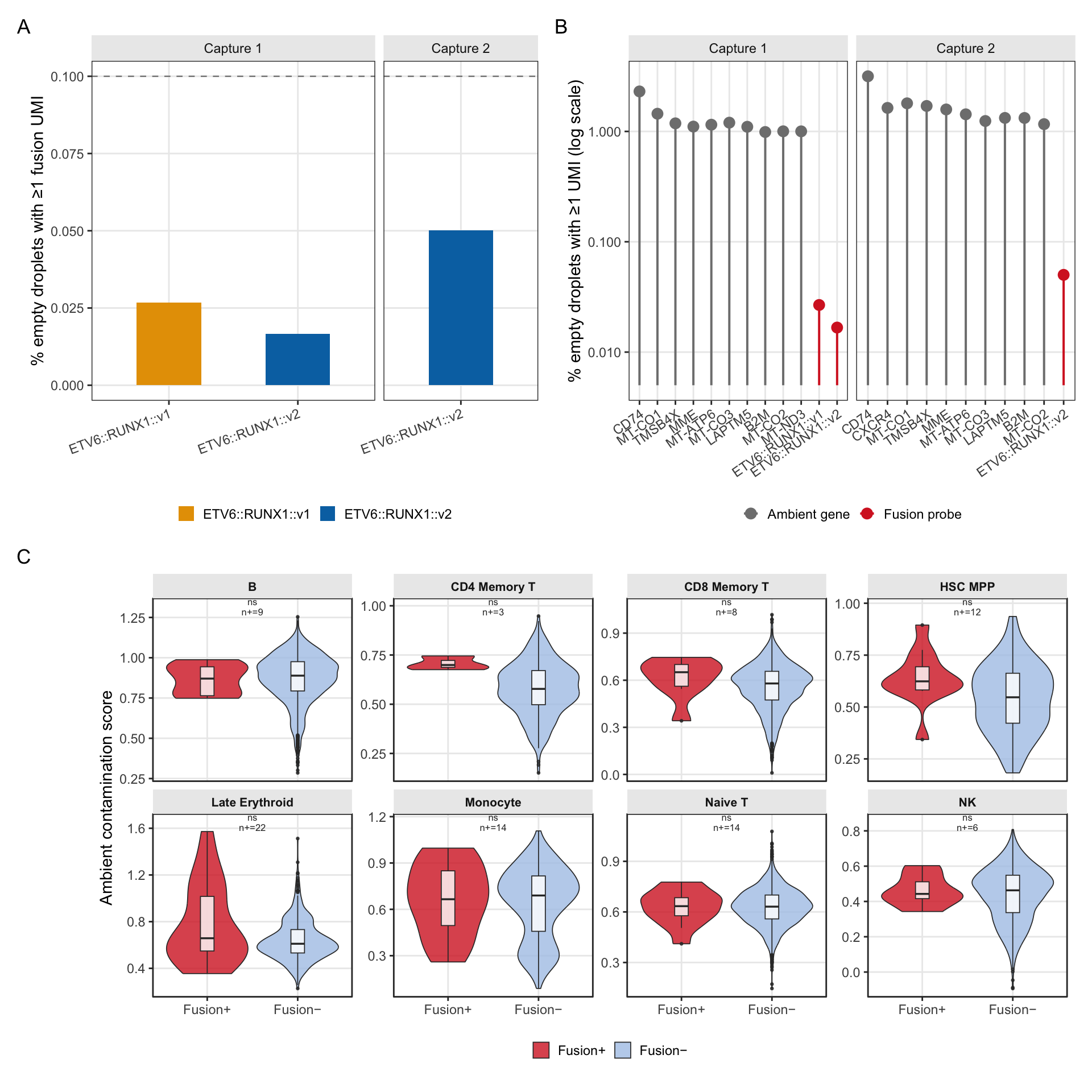
Session info
sessioninfo::session_info()─ Session info ───────────────────────────────────────────────────────────────
setting value
version R version 4.4.1 (2024-06-14)
os macOS 15.5
system aarch64, darwin20
ui X11
language (EN)
collate en_US.UTF-8
ctype en_US.UTF-8
tz Australia/Melbourne
date 2026-07-16
pandoc 3.8.3 @ /Applications/RStudio.app/Contents/Resources/app/quarto/bin/tools/aarch64/ (via rmarkdown)
quarto 1.9.38 @ /Applications/RStudio.app/Contents/Resources/app/quarto/bin/quarto
─ Packages ───────────────────────────────────────────────────────────────────
! package * version date (UTC) lib source
P abind 1.4-8 2024-09-12 [?] CRAN (R 4.4.1)
P beachmat 2.22.0 2024-11-08 [?] Bioconduc~
P Biobase * 2.66.0 2024-11-08 [?] Bioconduc~
P BiocGenerics * 0.52.0 2024-11-08 [?] Bioconduc~
P BiocManager 1.30.27 2025-11-14 [?] CRAN (R 4.4.3)
P BiocParallel 1.40.2 2025-04-08 [?] Bioconductor
P bslib 0.9.0 2025-01-30 [?] CRAN (R 4.4.1)
P cachem 1.1.0 2024-05-16 [?] CRAN (R 4.4.1)
P callr 3.7.6 2024-03-25 [?] CRAN (R 4.4.0)
P cli 3.6.5 2025-04-23 [?] CRAN (R 4.4.1)
P cluster 2.1.6 2023-12-01 [?] CRAN (R 4.4.1)
P codetools 0.2-20 2024-03-31 [?] CRAN (R 4.4.1)
P colorspace 2.1-1 2024-07-26 [?] CRAN (R 4.4.1)
P cowplot 1.1.3 2024-01-22 [?] CRAN (R 4.4.0)
P crayon 1.5.3 2024-06-20 [?] CRAN (R 4.4.1)
P data.table 1.18.2.1 2026-01-27 [?] CRAN (R 4.4.3)
P DelayedArray 0.32.0 2024-11-08 [?] Bioconduc~
P DelayedMatrixStats 1.28.1 2025-01-09 [?] Bioconduc~
P deldir 2.0-4 2024-02-28 [?] CRAN (R 4.4.1)
P digest 0.6.37 2024-08-19 [?] CRAN (R 4.4.1)
P dotCall64 1.2 2024-10-04 [?] CRAN (R 4.4.1)
P dplyr * 1.1.4 2023-11-17 [?] CRAN (R 4.4.0)
P dqrng 0.4.1 2024-05-28 [?] CRAN (R 4.4.0)
P DropletUtils * 1.26.0 2024-11-08 [?] Bioconduc~
P edgeR 4.4.2 2025-01-27 [?] Bioconduc~
P evaluate 1.0.3 2025-01-10 [?] CRAN (R 4.4.1)
P farver 2.1.2 2024-05-13 [?] CRAN (R 4.4.1)
P fastDummies 1.7.5 2025-01-20 [?] CRAN (R 4.4.1)
P fastmap 1.2.0 2024-05-15 [?] CRAN (R 4.4.1)
P fitdistrplus 1.2-2 2025-01-07 [?] CRAN (R 4.4.1)
P forcats * 1.0.0 2023-01-29 [?] CRAN (R 4.4.0)
P fs 1.6.6 2025-04-12 [?] CRAN (R 4.4.1)
P future 1.49.0 2025-05-09 [?] CRAN (R 4.4.1)
P future.apply 1.11.3 2024-10-27 [?] CRAN (R 4.4.1)
P generics 0.1.4 2025-05-09 [?] CRAN (R 4.4.1)
P GenomeInfoDb * 1.42.3 2025-01-27 [?] Bioconduc~
P GenomeInfoDbData 1.2.13 2025-05-28 [?] Bioconductor
P GenomicRanges * 1.58.0 2024-11-08 [?] Bioconduc~
P getPass 0.2-4 2023-12-10 [?] CRAN (R 4.4.1)
P ggplot2 * 4.0.2 2026-02-03 [?] CRAN (R 4.4.3)
P ggrepel * 0.9.6 2024-09-07 [?] CRAN (R 4.4.1)
P ggridges 0.5.6 2024-01-23 [?] CRAN (R 4.4.0)
P git2r 0.36.2 2025-03-29 [?] CRAN (R 4.4.1)
P globals 0.18.0 2025-05-08 [?] CRAN (R 4.4.1)
P glue * 1.8.0 2024-09-30 [?] CRAN (R 4.4.1)
P goftest 1.2-3 2021-10-07 [?] CRAN (R 4.4.1)
P gridExtra 2.3 2017-09-09 [?] CRAN (R 4.4.1)
P gtable 0.3.6 2024-10-25 [?] CRAN (R 4.4.1)
P HDF5Array 1.34.0 2024-11-08 [?] Bioconduc~
P here * 1.0.1 2020-12-13 [?] CRAN (R 4.4.1)
P hms 1.1.3 2023-03-21 [?] CRAN (R 4.4.0)
P htmltools 0.5.8.1 2024-04-04 [?] CRAN (R 4.4.1)
P htmlwidgets 1.6.4 2023-12-06 [?] CRAN (R 4.4.0)
P httpuv 1.6.16 2025-04-16 [?] CRAN (R 4.4.1)
P httr 1.4.7 2023-08-15 [?] CRAN (R 4.4.0)
P ica 1.0-3 2022-07-08 [?] CRAN (R 4.4.1)
P igraph 2.1.4 2025-01-23 [?] CRAN (R 4.4.1)
P IRanges * 2.40.1 2024-12-05 [?] Bioconduc~
P irlba 2.3.5.1 2022-10-03 [?] CRAN (R 4.4.0)
P jquerylib 0.1.4 2021-04-26 [?] CRAN (R 4.4.0)
P jsonlite 2.0.0 2025-03-27 [?] CRAN (R 4.4.1)
P KernSmooth 2.23-24 2024-05-17 [?] CRAN (R 4.4.1)
P knitr 1.50 2025-03-16 [?] CRAN (R 4.4.1)
P labeling 0.4.3 2023-08-29 [?] CRAN (R 4.4.1)
P later 1.4.2 2025-04-08 [?] CRAN (R 4.4.1)
P lattice 0.22-6 2024-03-20 [?] CRAN (R 4.4.1)
P lazyeval 0.2.2 2019-03-15 [?] CRAN (R 4.4.1)
P lifecycle 1.0.4 2023-11-07 [?] CRAN (R 4.4.1)
P limma 3.62.2 2025-01-09 [?] Bioconduc~
P listenv 0.9.1 2024-01-29 [?] CRAN (R 4.4.1)
P lmtest 0.9-40 2022-03-21 [?] CRAN (R 4.4.1)
P locfit 1.5-9.12 2025-03-05 [?] CRAN (R 4.4.1)
P lubridate * 1.9.4 2024-12-08 [?] CRAN (R 4.4.1)
P magrittr 2.0.3 2022-03-30 [?] CRAN (R 4.4.1)
P MASS 7.3-60.2 2024-04-26 [?] CRAN (R 4.4.1)
P Matrix 1.7-0 2024-04-26 [?] CRAN (R 4.4.1)
P MatrixGenerics * 1.18.1 2025-01-09 [?] Bioconduc~
P matrixStats * 1.5.0 2025-01-07 [?] CRAN (R 4.4.1)
P mime 0.13 2025-03-17 [?] CRAN (R 4.4.1)
P miniUI 0.1.2 2025-04-17 [?] CRAN (R 4.4.1)
P nlme 3.1-164 2023-11-27 [?] CRAN (R 4.4.1)
P parallelly 1.45.0 2025-06-02 [?] CRAN (R 4.4.1)
P patchwork * 1.3.0 2024-09-16 [?] CRAN (R 4.4.1)
P pbapply 1.7-4 2025-07-20 [?] CRAN (R 4.4.1)
P pillar 1.10.2 2025-04-05 [?] CRAN (R 4.4.1)
P pkgconfig 2.0.3 2019-09-22 [?] CRAN (R 4.4.1)
P plotly 4.10.4 2024-01-13 [?] CRAN (R 4.4.0)
P plyr 1.8.9 2023-10-02 [?] CRAN (R 4.4.1)
P png 0.1-8 2022-11-29 [?] CRAN (R 4.4.1)
P polyclip 1.10-7 2024-07-23 [?] CRAN (R 4.4.1)
P processx 3.8.6 2025-02-21 [?] CRAN (R 4.4.1)
P progressr 0.15.1 2024-11-22 [?] CRAN (R 4.4.1)
P promises 1.3.3 2025-05-29 [?] CRAN (R 4.4.1)
P ps 1.9.1 2025-04-12 [?] CRAN (R 4.4.1)
P purrr * 1.0.4 2025-02-05 [?] CRAN (R 4.4.1)
P R.methodsS3 1.8.2 2022-06-13 [?] CRAN (R 4.4.1)
P R.oo 1.27.1 2025-05-02 [?] CRAN (R 4.4.1)
P R.utils 2.13.0 2025-02-24 [?] CRAN (R 4.4.1)
P R6 2.6.1 2025-02-15 [?] CRAN (R 4.4.1)
P RANN 2.6.2 2024-08-25 [?] CRAN (R 4.4.1)
P RColorBrewer 1.1-3 2022-04-03 [?] CRAN (R 4.4.1)
P Rcpp 1.1.1-1.1 2026-04-24 [?] CRAN (R 4.4.1)
P RcppAnnoy 0.0.22 2024-01-23 [?] CRAN (R 4.4.1)
P RcppHNSW 0.6.0 2024-02-04 [?] CRAN (R 4.4.1)
P readr * 2.1.5 2024-01-10 [?] CRAN (R 4.4.0)
renv 1.1.4 2025-03-20 [1] CRAN (R 4.4.1)
P reshape2 1.4.4 2020-04-09 [?] CRAN (R 4.4.0)
P reticulate 1.42.0 2025-03-25 [?] CRAN (R 4.4.1)
P rhdf5 2.50.2 2025-01-09 [?] Bioconduc~
P rhdf5filters 1.18.1 2025-03-06 [?] Bioconduc~
P Rhdf5lib 1.28.0 2024-11-08 [?] Bioconduc~
P rlang 1.1.6 2025-04-11 [?] CRAN (R 4.4.1)
P rmarkdown 2.29 2024-11-04 [?] CRAN (R 4.4.1)
P ROCR 1.0-11 2020-05-02 [?] CRAN (R 4.4.0)
P rprojroot 2.0.4 2023-11-05 [?] CRAN (R 4.4.1)
P RSpectra 0.16-2 2024-07-18 [?] CRAN (R 4.4.0)
P rstudioapi 0.17.1 2024-10-22 [?] CRAN (R 4.4.1)
P Rtsne 0.17 2023-12-07 [?] CRAN (R 4.4.1)
P S4Arrays 1.6.0 2024-11-08 [?] Bioconduc~
P S4Vectors * 0.44.0 2024-11-08 [?] Bioconduc~
P S7 0.2.0 2024-11-07 [?] CRAN (R 4.4.1)
P sass 0.4.10 2025-04-11 [?] CRAN (R 4.4.1)
P scales * 1.4.0 2025-04-24 [?] CRAN (R 4.4.1)
P scattermore 1.2 2023-06-12 [?] CRAN (R 4.4.0)
P sctransform 0.4.2 2025-04-30 [?] CRAN (R 4.4.1)
P scuttle 1.16.0 2024-11-08 [?] Bioconduc~
P sessioninfo 1.2.3 2025-02-05 [?] CRAN (R 4.4.1)
P Seurat * 5.3.0 2025-04-23 [?] CRAN (R 4.4.1)
P SeuratObject * 5.1.0 2025-04-22 [?] CRAN (R 4.4.1)
P shiny 1.10.0 2024-12-14 [?] CRAN (R 4.4.1)
P SingleCellExperiment * 1.28.1 2024-11-23 [?] Bioconduc~
P sp * 2.2-0 2025-02-01 [?] CRAN (R 4.4.1)
P spam 2.11-1 2025-01-20 [?] CRAN (R 4.4.1)
P SparseArray 1.6.2 2025-02-20 [?] Bioconduc~
P sparseMatrixStats 1.18.0 2024-11-08 [?] Bioconduc~
P spatstat.data 3.1-6 2025-03-17 [?] CRAN (R 4.4.1)
P spatstat.explore 3.4-3 2025-05-21 [?] CRAN (R 4.4.1)
P spatstat.geom 3.4-1 2025-05-20 [?] CRAN (R 4.4.1)
P spatstat.random 3.4-1 2025-05-20 [?] CRAN (R 4.4.1)
P spatstat.sparse 3.1-0 2024-06-21 [?] CRAN (R 4.4.0)
P spatstat.univar 3.1-3 2025-05-08 [?] CRAN (R 4.4.1)
P spatstat.utils 3.1-4 2025-05-15 [?] CRAN (R 4.4.1)
P statmod 1.5.0 2023-01-06 [?] CRAN (R 4.4.1)
P stringi 1.8.7 2025-03-27 [?] CRAN (R 4.4.1)
P stringr * 1.6.0 2025-11-04 [?] CRAN (R 4.4.1)
P SummarizedExperiment * 1.36.0 2024-11-08 [?] Bioconduc~
P survival 3.6-4 2024-04-24 [?] CRAN (R 4.4.1)
P tensor 1.5 2012-05-05 [?] CRAN (R 4.4.1)
P tibble * 3.2.1 2023-03-20 [?] CRAN (R 4.4.0)
P tidyr * 1.3.1 2024-01-24 [?] CRAN (R 4.4.1)
P tidyselect 1.2.1 2024-03-11 [?] CRAN (R 4.4.0)
P tidyverse * 2.0.0 2023-02-22 [?] CRAN (R 4.4.0)
P timechange 0.3.0 2024-01-18 [?] CRAN (R 4.4.1)
P tzdb 0.5.0 2025-03-15 [?] CRAN (R 4.4.1)
P UCSC.utils 1.2.0 2024-11-08 [?] Bioconduc~
P utf8 1.2.5 2025-05-01 [?] CRAN (R 4.4.1)
P uwot 0.2.3 2025-02-24 [?] CRAN (R 4.4.1)
P vctrs 0.6.5 2023-12-01 [?] CRAN (R 4.4.0)
P viridisLite 0.4.2 2023-05-02 [?] CRAN (R 4.4.1)
P whisker 0.4.1 2022-12-05 [?] CRAN (R 4.4.1)
P withr 3.0.2 2024-10-28 [?] CRAN (R 4.4.1)
P workflowr * 1.7.1 2023-08-23 [?] CRAN (R 4.4.0)
P xfun 0.56 2026-01-18 [?] CRAN (R 4.4.3)
P xtable 1.8-4 2019-04-21 [?] CRAN (R 4.4.1)
P XVector 0.46.0 2024-11-08 [?] Bioconduc~
P yaml 2.3.10 2024-07-26 [?] CRAN (R 4.4.1)
P zlibbioc 1.52.0 2024-11-08 [?] Bioconduc~
P zoo 1.8-14 2025-04-10 [?] CRAN (R 4.4.1)
[1] /Users/maksimovicjovana/projects/active/flex-fusion-probes/renv/library/macos/R-4.4/aarch64-apple-darwin20
[2] /Users/maksimovicjovana/Library/Caches/org.R-project.R/R/renv/sandbox/macos/R-4.4/aarch64-apple-darwin20/f7156815
* ── Packages attached to the search path.
P ── Loaded and on-disk path mismatch.
──────────────────────────────────────────────────────────────────────────────
sessionInfo()R version 4.4.1 (2024-06-14)
Platform: aarch64-apple-darwin20
Running under: macOS 15.5
Matrix products: default
BLAS: /Library/Frameworks/R.framework/Versions/4.4-arm64/Resources/lib/libRblas.0.dylib
LAPACK: /Library/Frameworks/R.framework/Versions/4.4-arm64/Resources/lib/libRlapack.dylib; LAPACK version 3.12.0
locale:
[1] en_US.UTF-8/en_US.UTF-8/en_US.UTF-8/C/en_US.UTF-8/en_US.UTF-8
time zone: Australia/Melbourne
tzcode source: internal
attached base packages:
[1] stats4 stats graphics grDevices datasets utils methods
[8] base
other attached packages:
[1] scales_1.4.0 glue_1.8.0
[3] here_1.0.1 ggrepel_0.9.6
[5] patchwork_1.3.0 lubridate_1.9.4
[7] forcats_1.0.0 stringr_1.6.0
[9] dplyr_1.1.4 purrr_1.0.4
[11] readr_2.1.5 tidyr_1.3.1
[13] tibble_3.2.1 ggplot2_4.0.2
[15] tidyverse_2.0.0 DropletUtils_1.26.0
[17] SingleCellExperiment_1.28.1 SummarizedExperiment_1.36.0
[19] Biobase_2.66.0 GenomicRanges_1.58.0
[21] GenomeInfoDb_1.42.3 IRanges_2.40.1
[23] S4Vectors_0.44.0 BiocGenerics_0.52.0
[25] MatrixGenerics_1.18.1 matrixStats_1.5.0
[27] Seurat_5.3.0 SeuratObject_5.1.0
[29] sp_2.2-0 workflowr_1.7.1
loaded via a namespace (and not attached):
[1] RcppAnnoy_0.0.22 splines_4.4.1
[3] later_1.4.2 R.oo_1.27.1
[5] polyclip_1.10-7 fastDummies_1.7.5
[7] lifecycle_1.0.4 edgeR_4.4.2
[9] rprojroot_2.0.4 globals_0.18.0
[11] processx_3.8.6 lattice_0.22-6
[13] MASS_7.3-60.2 magrittr_2.0.3
[15] limma_3.62.2 plotly_4.10.4
[17] sass_0.4.10 rmarkdown_2.29
[19] jquerylib_0.1.4 yaml_2.3.10
[21] httpuv_1.6.16 sctransform_0.4.2
[23] spam_2.11-1 sessioninfo_1.2.3
[25] spatstat.sparse_3.1-0 reticulate_1.42.0
[27] cowplot_1.1.3 pbapply_1.7-4
[29] RColorBrewer_1.1-3 abind_1.4-8
[31] zlibbioc_1.52.0 Rtsne_0.17
[33] R.utils_2.13.0 git2r_0.36.2
[35] GenomeInfoDbData_1.2.13 irlba_2.3.5.1
[37] listenv_0.9.1 spatstat.utils_3.1-4
[39] goftest_1.2-3 RSpectra_0.16-2
[41] spatstat.random_3.4-1 dqrng_0.4.1
[43] fitdistrplus_1.2-2 parallelly_1.45.0
[45] DelayedMatrixStats_1.28.1 codetools_0.2-20
[47] DelayedArray_0.32.0 scuttle_1.16.0
[49] tidyselect_1.2.1 UCSC.utils_1.2.0
[51] farver_2.1.2 spatstat.explore_3.4-3
[53] jsonlite_2.0.0 progressr_0.15.1
[55] ggridges_0.5.6 survival_3.6-4
[57] tools_4.4.1 ica_1.0-3
[59] Rcpp_1.1.1-1.1 gridExtra_2.3
[61] SparseArray_1.6.2 xfun_0.56
[63] HDF5Array_1.34.0 withr_3.0.2
[65] BiocManager_1.30.27 fastmap_1.2.0
[67] rhdf5filters_1.18.1 callr_3.7.6
[69] digest_0.6.37 timechange_0.3.0
[71] R6_2.6.1 mime_0.13
[73] colorspace_2.1-1 scattermore_1.2
[75] tensor_1.5 spatstat.data_3.1-6
[77] R.methodsS3_1.8.2 utf8_1.2.5
[79] generics_0.1.4 renv_1.1.4
[81] data.table_1.18.2.1 httr_1.4.7
[83] htmlwidgets_1.6.4 S4Arrays_1.6.0
[85] whisker_0.4.1 uwot_0.2.3
[87] pkgconfig_2.0.3 gtable_0.3.6
[89] lmtest_0.9-40 S7_0.2.0
[91] XVector_0.46.0 htmltools_0.5.8.1
[93] dotCall64_1.2 png_0.1-8
[95] spatstat.univar_3.1-3 knitr_1.50
[97] rstudioapi_0.17.1 tzdb_0.5.0
[99] reshape2_1.4.4 nlme_3.1-164
[101] cachem_1.1.0 zoo_1.8-14
[103] rhdf5_2.50.2 KernSmooth_2.23-24
[105] parallel_4.4.1 miniUI_0.1.2
[107] pillar_1.10.2 grid_4.4.1
[109] vctrs_0.6.5 RANN_2.6.2
[111] promises_1.3.3 beachmat_2.22.0
[113] xtable_1.8-4 cluster_2.1.6
[115] evaluate_1.0.3 locfit_1.5-9.12
[117] cli_3.6.5 compiler_4.4.1
[119] rlang_1.1.6 crayon_1.5.3
[121] future.apply_1.11.3 labeling_0.4.3
[123] ps_1.9.1 getPass_0.2-4
[125] plyr_1.8.9 fs_1.6.6
[127] stringi_1.8.7 viridisLite_0.4.2
[129] deldir_2.0-4 BiocParallel_1.40.2
[131] lazyeval_0.2.2 spatstat.geom_3.4-1
[133] Matrix_1.7-0 RcppHNSW_0.6.0
[135] hms_1.1.3 sparseMatrixStats_1.18.0
[137] future_1.49.0 Rhdf5lib_1.28.0
[139] statmod_1.5.0 shiny_1.10.0
[141] ROCR_1.0-11 igraph_2.1.4
[143] bslib_0.9.0