B-ALL Experiment 2: Quality Control
Cell calling, mito% filtering, doublet removal, and Supplementary Figure 4 assembly
Jovana Maksimovic
August 25, 2026
Last updated: 2026-08-25
Checks: 7 0
Knit directory: flex-fusion-probes/
This reproducible R Markdown analysis was created with workflowr (version 1.7.1). The Checks tab describes the reproducibility checks that were applied when the results were created. The Past versions tab lists the development history.
Great! Since the R Markdown file has been committed to the Git repository, you know the exact version of the code that produced these results.
Great job! The global environment was empty. Objects defined in the global environment can affect the analysis in your R Markdown file in unknown ways. For reproduciblity it’s best to always run the code in an empty environment.
The command set.seed(20240925) was run prior to running
the code in the R Markdown file. Setting a seed ensures that any results
that rely on randomness, e.g. subsampling or permutations, are
reproducible.
Great job! Recording the operating system, R version, and package versions is critical for reproducibility.
Nice! There were no cached chunks for this analysis, so you can be confident that you successfully produced the results during this run.
Great job! Using relative paths to the files within your workflowr project makes it easier to run your code on other machines.
Great! You are using Git for version control. Tracking code development and connecting the code version to the results is critical for reproducibility.
The results in this page were generated with repository version 528a938. See the Past versions tab to see a history of the changes made to the R Markdown and HTML files.
Note that you need to be careful to ensure that all relevant files for
the analysis have been committed to Git prior to generating the results
(you can use wflow_publish or
wflow_git_commit). workflowr only checks the R Markdown
file, but you know if there are other scripts or data files that it
depends on. Below is the status of the Git repository when the results
were generated:
Ignored files:
    Ignored:    .DS_Store
    Ignored:    .Rhistory
    Ignored:    .Rproj.user/
    Ignored:    CLAUDE.md
    Ignored:    analysis/.gitignore
    Ignored:    analysis/B-ALL_exp2_nonblast_fusion_analysis_cache/
    Ignored:    analysis/obsolete/B-ALL_nonblast_fusion_analysis_cache/
    Ignored:    analysis/projectionFigures/
    Ignored:    code/files/
    Ignored:    data/.DS_Store
    Ignored:    data/BoneMarrowMap/
    Ignored:    data/BoneMarrowMapBoneMarrowMap_SymphonyReference.rds
    Ignored:    data/BoneMarrowMapBoneMarrowMap_uwot_model.uwot
    Ignored:    data/CAPTURE-1-POOL-FLEX/
    Ignored:    data/CAPTURE-2-POOL-FLEX/
    Ignored:    data/Pool-240917-FLEX/
    Ignored:    data/RDS/
    Ignored:    data/Run_1_and_Run_2/
    Ignored:    data/Run_2/
    Ignored:    data/victoria_stuff/
    Ignored:    logs/
    Ignored:    methods_updated.md
    Ignored:    output/
    Ignored:    projectionFigures/
    Ignored:    renv/library/
    Ignored:    renv/staging/

Untracked files:
    Untracked:  _to_delete/
    Untracked:  data/Config_Sample_CAPTURE-1-POOL-FLEX.csv
    Untracked:  data/Config_Sample_CAPTURE-2-POOL-FLEX.csv
    Untracked:  data/Config_Sample_Pool-240917-FLEX.csv
    Untracked:  data/cellranger-multi_flex_fusions_pool_1.sbatch
    Untracked:  data/cellranger-multi_flex_fusions_pool_2.sbatch

Unstaged changes:
    Modified:   .gitignore
    Modified:   render_all.sh

Staged changes:
    Modified:   data/sample_information_flex_experiment_2.csv
Note that any generated files, e.g. HTML, png, CSS, etc., are not included in this status report because it is ok for generated content to have uncommitted changes.
These are the previous versions of the repository in which changes were
made to the R Markdown
(analysis/B-ALL_exp2_quality_control.Rmd) and HTML
(docs/B-ALL_exp2_quality_control.html) files. If you’ve
configured a remote Git repository (see ?wflow_git_remote),
click on the hyperlinks in the table below to view the files as they
were in that past version.
| File | Version | Author | Date | Message |
|---|---|---|---|---|
| html | b5bcfc1 | Jovana Maksimovic | 2026-08-25 | Build site. |
| html | 0460f4e | Jovana Maksimovic | 2026-08-25 | Build site. |
| html | d63b2ed | Jovana Maksimovic | 2026-07-15 | Build site. |
| Rmd | cfadb5d | Jovana Maksimovic | 2026-07-15 | wflow_publish("analysis/B-ALL_exp2_quality_control.Rmd") |
| html | abab370 | Jovana Maksimovic | 2026-05-19 | Build site. |
| Rmd | 5481825 | Jovana Maksimovic | 2026-05-19 | Update figure labels, add C369 heading, comment out exp1 DE section, minor point size |
| html | 1b5bb97 | Jovana Maksimovic | 2026-05-11 | Build site. |
| Rmd | 1f3159b | Jovana Maksimovic | 2026-05-08 | Rename RDS checkpoints to systematic naming scheme |
| Rmd | 71c5f99 | Jovana Maksimovic | 2026-05-08 | docs: add getting_started page; fix myeloid_types error; move exploratory notebooks to obsolete |
| Rmd | 1578018 | Jovana Maksimovic | 2026-05-08 | docs: add prose, standardise headings and figure labels across all 10 B-ALL notebooks |
| Rmd | 1a33400 | Jovana Maksimovic | 2026-05-08 | B-ALL cleanup: fix index links, stray library() calls, add chunk labels |
| Rmd | 1724beb | Jovana Maksimovic | 2026-05-08 | Standardise YAML headers and chunk names across all notebooks; merge utility_functions into utilities.R |
| Rmd | 10d2f5e | Jovana Maksimovic | 2026-05-08 | Rename analysis notebooks to new naming scheme |
This notebook performs quality control for Experiment 2 B-ALL patient
samples, which were sequenced across two captures (Capture 1:
C1437_Diagnosis, C1437_Relapse, C369_Diagnosis, C659_Diagnosis; Capture
2: C369_MRD, C369_Relapse, C601_Diagnosis, C658_Diagnosis). The two
captures differ substantially in sequencing depth (~4,085 vs. ~22,877
reads/cell). Cell calling uses emptyDrops() (FDR <
0.001) combined with CellRanger knee-point calls (union), run separately
per capture on the raw feature-barcode matrices. Cells are then filtered
based on mitochondrial read percentage and doublets are identified using
scDblFinder. The full QC summary figure is assembled as
Supplementary Figure 4 at the end of this notebook.
Load data
# ── Discover samples from directory structure ─────────────────────────────────
captures <- c("CAPTURE-1-POOL-FLEX", "CAPTURE-2-POOL-FLEX")

sample_data <- do.call(rbind, lapply(captures, function(cap) {
  base_dir <- here("data", "Run_1_and_Run_2",
                   paste0("Cellranger_Config_Sample_", cap),
                   "outs", "per_sample_outs")

  samples <- list.files(base_dir)

  data.frame(
    capture = cap,
    sample  = samples,
    dir     = file.path(base_dir, samples, "count",
                        "sample_filtered_feature_bc_matrix"),
    stringsAsFactors = FALSE
  )
}))

# ── Verify all paths exist ────────────────────────────────────────────────────
cat("Samples found:\n")
Samples found:for (i in seq_len(nrow(sample_data))) {
cat(sample_data$sample[i], "—",
ifelse(dir.exists(sample_data$dir[i]), "EXISTS", "MISSING"), "\n")
}CAPTURE-1-POOL-FLEX_Sample-1 — EXISTS
CAPTURE-1-POOL-FLEX_Sample-2 — EXISTS
CAPTURE-1-POOL-FLEX_Sample-3 — EXISTS
CAPTURE-1-POOL-FLEX_Sample-4 — EXISTS
CAPTURE-2-POOL-FLEX_Sample-1 — EXISTS
CAPTURE-2-POOL-FLEX_Sample-2 — EXISTS
CAPTURE-2-POOL-FLEX_Sample-3 — EXISTS
CAPTURE-2-POOL-FLEX_Sample-4 — EXISTS emptyDrops() is run separately on each capture’s raw
matrix and the result is cached. Delete
exp2_emptydrops.sce.rds to force a fresh run.
ed_rds <- here("data", "RDS", "exp2_emptydrops.sce.rds")

if (file.exists(ed_rds)) {
  cat("Loading cached emptyDrops result ...\n")
  sce_ed <- readRDS(ed_rds)
} else {
  # ── Per-capture raw and per-sample directories ────────────────────────────────
  capture_dirs <- list(
    "CAPTURE-1-POOL-FLEX" = list(
      raw_dir = here("data", "CAPTURE-1-POOL-FLEX",
                     "outs", "multi", "count", "raw_feature_bc_matrix"),
      ps_dir  = here("data", "CAPTURE-1-POOL-FLEX",
                     "outs", "per_sample_outs")
    ),
    "CAPTURE-2-POOL-FLEX" = list(
      raw_dir = here("data", "Run_1_and_Run_2",
                     "Cellranger_Config_Sample_CAPTURE-2-POOL-FLEX",
                     "outs", "multi", "count", "raw_feature_bc_matrix"),
      ps_dir  = here("data", "Run_1_and_Run_2",
                     "Cellranger_Config_Sample_CAPTURE-2-POOL-FLEX",
                     "outs", "per_sample_outs")
    )
  )

  # ── Helper: collect CellRanger filtered barcodes ──────────────────────────────
  get_filtered_bc <- function(ps_dir) {
    unlist(lapply(
      list.dirs(ps_dir, full.names = TRUE, recursive = FALSE),
      function(d) {
        bc_file <- file.path(d, "count", "sample_filtered_feature_bc_matrix",
                             "barcodes.tsv.gz")
        if (file.exists(bc_file)) readLines(gzcon(file(bc_file, "rb")))
      }
    ), use.names = FALSE)
  }

  # ── Helper: assign Sample (directory name) from probe barcode ─────────────────
  assign_sample_label <- function(sce, ps_dir) {
    sample_dirs <- sort(list.dirs(ps_dir, full.names = TRUE, recursive = FALSE))
    probe_bcs   <- sapply(sample_dirs, function(d) {
      bc_file <- file.path(d, "count", "sample_filtered_feature_bc_matrix",
                           "barcodes.tsv.gz")
      bc     <- readLines(gzcon(file(bc_file, "rb")))[1]
      bc_seq <- sub("-[0-9]+$", "", bc)
      substr(bc_seq, nchar(bc_seq) - 7L, nchar(bc_seq))
    })
    probe_map <- data.frame(probe_bc = unname(probe_bcs),
                            sample   = basename(sample_dirs),
                            stringsAsFactors = FALSE)
    bc_seq   <- sub("-[0-9]+$", "", colnames(sce))
    pbc      <- substr(bc_seq, nchar(bc_seq) - 7L, nchar(bc_seq))
    idx      <- match(pbc, probe_map$probe_bc)
    sce$Sample <- probe_map$sample[idx]
    sce[, !is.na(sce$Sample)]
  }

  # ── Run emptyDrops per capture ────────────────────────────────────────────────
  cap_sces <- lapply(names(capture_dirs), function(cap_name) {
    cap <- capture_dirs[[cap_name]]
    cat(glue("\nProcessing {cap_name} ...\n"))

    filtered_bc <- get_filtered_bc(cap$ps_dir)

    cat("  Loading raw matrix ...\n")
    raw_sce <- read10xCounts(cap$raw_dir, col.names = TRUE)

    cat("  Running emptyDrops (FDR < 0.001) ...\n")
    set.seed(100)
    ed_out  <- emptyDrops(counts(raw_sce))
    ed_sig  <- rownames(ed_out)[!is.na(ed_out$FDR) & ed_out$FDR < 0.001]
    keep_bc <- union(filtered_bc, intersect(colnames(raw_sce), ed_sig))
    cap_sce <- raw_sce[, colnames(raw_sce) %in% keep_bc]
    cap_sce <- assign_sample_label(cap_sce, cap$ps_dir)

    cat(glue("  Cells retained: {ncol(cap_sce)}\n"))
    print(table(cap_sce$Sample))
    cap_sce
  })

  # ── Combine captures; suffix barcodes to ensure uniqueness across captures ────
  suffixes <- c("_cap1", "_cap2")
  for (i in seq_along(cap_sces)) {
    colnames(cap_sces[[i]]) <- paste0(colnames(cap_sces[[i]]), suffixes[i])
  }
  sce_ed <- do.call(cbind, cap_sces)

  cat(glue("\nTotal cells across both captures: {ncol(sce_ed)}\n"))

  saveRDS(sce_ed, ed_rds)
  cat(glue("Cached to {ed_rds}\n"))
}
Loading cached emptyDrops result ...sce <- logNormCounts(sce_ed)
sceclass: SingleCellExperiment
dim: 37145 106550
metadata(2): Samples Samples
assays(2): counts logcounts
rownames(37145): ENSG00000243485 ENSG00000237613 ...
DEPRECATED_ENSG00000284873 DEPRECATED_ENSG00000285687
rowData names(3): ID Symbol Type
colnames(106550): AAACAAGCAACCCTATATGTTGAC-1_cap1
AAACAAGCAACGACTAAACGGGAA-1_cap1 ... TTTGTGAGTGCTGATTAACGGGAA-1_cap2
TTTGTGAGTTAAGTCCACTTTAGG-1_cap2
colData names(3): Sample Barcode sizeFactor
reducedDimNames(0):
mainExpName: NULL
altExpNames(0):Add sample metadata.
sample_info <- read_csv(file = here("data/sample_information_flex_experiment_2.csv"))
colData(sce) %>%
  data.frame %>%
  left_join(sample_info %>%
              mutate(PPID = str_replace_all(PPID, "\\s+", ""),
                     patient_timepoint = paste0(PPID, "_", timepoint)),
            by = c("Sample" = "sample_id")) %>%
  DataFrame() -> colData(sce)

head(colData(sce)) %>%
knitr::kable()| Sample | Barcode | sizeFactor | PPID | timepoint | status | percent_blasts_in_bone_marrow | final_labelling | sample_name_for_single.cell | batch | patient_timepoint |
|---|---|---|---|---|---|---|---|---|---|---|
| CAPTURE-1-POOL-FLEX_Sample-4 | AAACAAGCAACCCTATATGTTGAC-1 | 0.5673976 | C659 | Diagnosis | LR | 95 | 4 | FLEX #6 GEMx 3’ #4 | 1 | C659_Diagnosis |
| CAPTURE-1-POOL-FLEX_Sample-2 | AAACAAGCAACGACTAAACGGGAA-1 | 1.3173322 | C1437 | Relapse | LR | 85 | 2 | FLEX #2 GEMx3’ #2 | 1 | C1437_Relapse |
| CAPTURE-1-POOL-FLEX_Sample-3 | AAACAAGCAACGACTAAGTAGGCT-1 | 0.3464024 | C369 | Diagnosis | LR | 87 | 3 | FLEX #3 GEMx3’ #3 | 1 | C369_Diagnosis |
| CAPTURE-1-POOL-FLEX_Sample-1 | AAACAAGCAAGGAATAACTTTAGG-1 | 0.3054360 | C1437 | Diagnosis | LR | 94 | 1 | FLEX #1 GEMx3’ #1 | 1 | C1437_Diagnosis |
| CAPTURE-1-POOL-FLEX_Sample-2 | AAACAAGCAAGTTAACAACGGGAA-1 | 0.4890878 | C1437 | Relapse | LR | 85 | 2 | FLEX #2 GEMx3’ #2 | 1 | C1437_Relapse |
| CAPTURE-1-POOL-FLEX_Sample-3 | AAACAAGCAAGTTAACAGTAGGCT-1 | 0.1995367 | C369 | Diagnosis | LR | 87 | 3 | FLEX #3 GEMx3’ #3 | 1 | C369_Diagnosis |
Data overview
Non-empty droplets
Overview of cell counts per sample directly from CellRanger output, before any QC filtering.
p3 <- ggcells(sce) +
  geom_bar(aes(x = patient_timepoint, fill = PPID)) +
  coord_flip() +
  ylab("Number of droplets") +
  geom_text(stat = "count", aes(x = patient_timepoint,
                                label = after_stat(count)),
            hjust=1.5, size=3) +
  theme_bw()

p3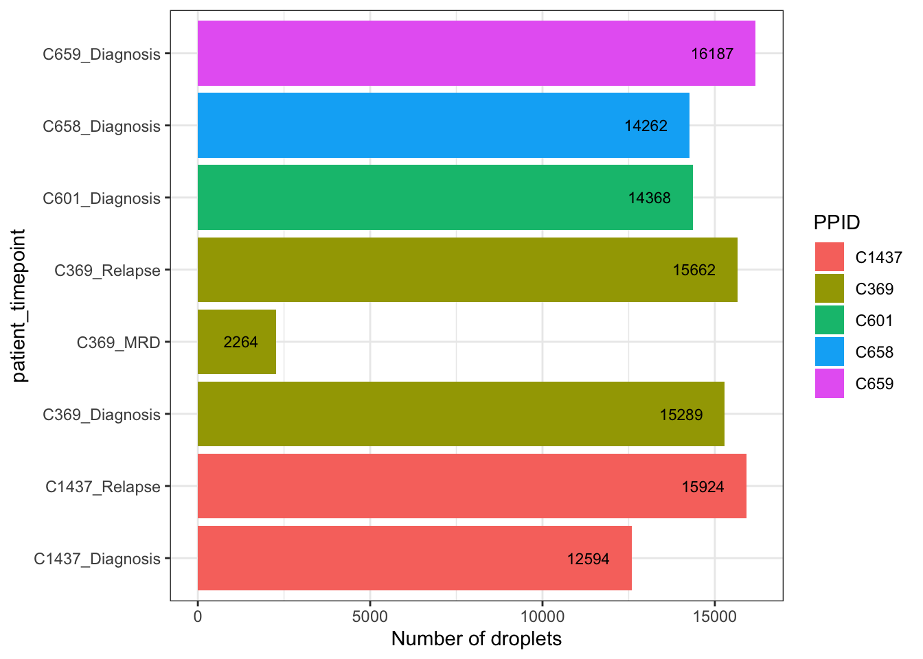
Fusion probe summary
Summary of reads mapping to custom fusion probe sequences. These probes detect the presence of specific chromosomal fusion transcripts at the single-cell level.
sce_fusions <- sce[grepl("fusion", rownames(sce)),]
sce_fusions
class: SingleCellExperiment
dim: 2 106550
metadata(2): Samples Samples
assays(2): counts logcounts
rownames(2): ETV6_RUNX1_v1_fusion ETV6_RUNX1_v2_fusion
rowData names(3): ID Symbol Type
colnames: NULL
colData names(11): Sample Barcode ... batch patient_timepoint
reducedDimNames(0):
mainExpName: NULL
altExpNames(0):The number of fusions assayed is 2.
Per cell fusion summary
sce_fusions <- addPerCellQC(sce_fusions)The library size and number of fusion genes detected per cell in each sample.
p1 <- plotColData(
  sce_fusions,
  "sum",
  x = "Sample",
  colour_by = "PPID",
  point_size = 0.5) +
  scale_y_log10() +
  annotation_logticks(
    sides = "l",
    short = unit(0.03, "cm"),
    mid = unit(0.06, "cm"),
    long = unit(0.09, "cm"))

p2 <- plotColData(
  sce_fusions,
  "detected",
  x = "Sample",
  colour_by = "PPID",
  point_size = 0.5)

# Define the axis rotation theme
axis_theme <- theme(
  axis.text.x = element_text(angle = 90, hjust = 1, vjust = 0)
)

# Apply axis theme to each plot
p1 <- p1 + axis_theme
p2 <- p2 + axis_theme

# Combine with patchwork and set global legend position
combined <- p1 + p2 +
  plot_layout(guides = "collect", ncol = 2) +
  plot_annotation(
    theme = theme(
      legend.position = "bottom"
    )
  )

combined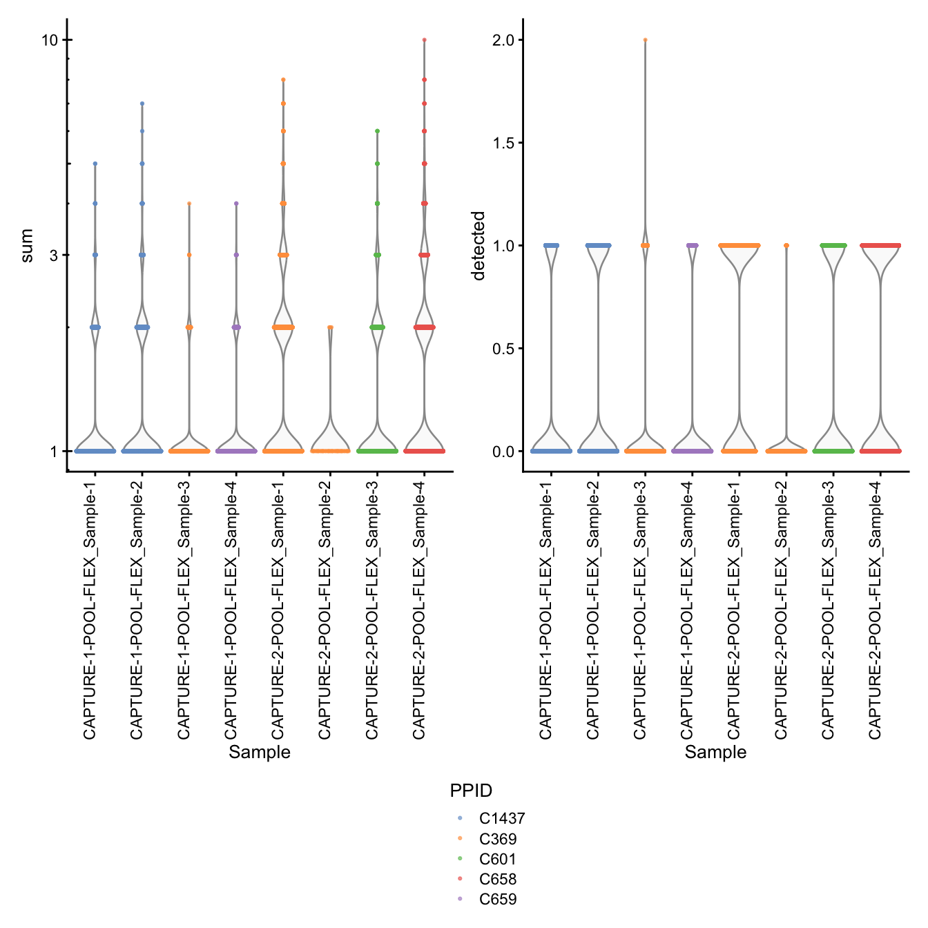
Total read counts per fusion
rowSums(counts(sce_fusions)) %>%
  as.data.frame %>%
  rownames_to_column(var = "Fusion") %>%
dplyr::rename("Total counts" = ".") %>% knitr::kable()| Fusion | Total counts |
|---|---|
| ETV6_RUNX1_v1_fusion | 11408 |
| ETV6_RUNX1_v2_fusion | 37881 |
Read count summary per fusion
sapply(1:nrow(sce_fusions), function(i){
  summary(counts(sce_fusions)[i,])
}) -> fusions_summary

colnames(fusions_summary) <- rownames(sce_fusions)
fusions_summary <- t(fusions_summary)
fusions_summary %>% knitr::kable()| Min. | 1st Qu. | Median | Mean | 3rd Qu. | Max. | |
|---|---|---|---|---|---|---|
| ETV6_RUNX1_v1_fusion | 0 | 0 | 0 | 0.1070671 | 0 | 7 |
| ETV6_RUNX1_v2_fusion | 0 | 0 | 0 | 0.3555232 | 0 | 10 |
No. cells expressing each fusion per sample
lapply(sample_data$sample, function(samp){
nexprs(sce_fusions[, sce_fusions$Sample == samp], byrow = TRUE) %>%
  as.data.frame() %>%
  rownames_to_column(var = "Fusion") %>%
  dplyr::rename("No. cells with counts > 0" = ".") %>%
    knitr::kable(caption = samp)
})
[[1]]
Table: CAPTURE-1-POOL-FLEX_Sample-1
|Fusion | No. cells with counts > 0|
|:--------------------|-------------------------:|
|ETV6_RUNX1_v1_fusion | 2908|
|ETV6_RUNX1_v2_fusion | 0|
[[2]]
Table: CAPTURE-1-POOL-FLEX_Sample-2
|Fusion | No. cells with counts > 0|
|:--------------------|-------------------------:|
|ETV6_RUNX1_v1_fusion | 5791|
|ETV6_RUNX1_v2_fusion | 0|
[[3]]
Table: CAPTURE-1-POOL-FLEX_Sample-3
|Fusion | No. cells with counts > 0|
|:--------------------|-------------------------:|
|ETV6_RUNX1_v1_fusion | 2|
|ETV6_RUNX1_v2_fusion | 1637|
[[4]]
Table: CAPTURE-1-POOL-FLEX_Sample-4
|Fusion | No. cells with counts > 0|
|:--------------------|-------------------------:|
|ETV6_RUNX1_v1_fusion | 0|
|ETV6_RUNX1_v2_fusion | 2658|
[[5]]
Table: CAPTURE-2-POOL-FLEX_Sample-1
|Fusion | No. cells with counts > 0|
|:--------------------|-------------------------:|
|ETV6_RUNX1_v1_fusion | 0|
|ETV6_RUNX1_v2_fusion | 8435|
[[6]]
Table: CAPTURE-2-POOL-FLEX_Sample-2
|Fusion | No. cells with counts > 0|
|:--------------------|-------------------------:|
|ETV6_RUNX1_v1_fusion | 0|
|ETV6_RUNX1_v2_fusion | 44|
[[7]]
Table: CAPTURE-2-POOL-FLEX_Sample-3
|Fusion | No. cells with counts > 0|
|:--------------------|-------------------------:|
|ETV6_RUNX1_v1_fusion | 0|
|ETV6_RUNX1_v2_fusion | 5371|
[[8]]
Table: CAPTURE-2-POOL-FLEX_Sample-4
|Fusion | No. cells with counts > 0|
|:--------------------|-------------------------:|
|ETV6_RUNX1_v1_fusion | 0|
|ETV6_RUNX1_v2_fusion | 7045|Fusion expression per sample
fusions <- str_detect(rownames(sce), "fusion")
plotExpression(sce,
               rownames(sce)[fusions],
               x = "patient_timepoint",
               colour_by = "PPID",
               scattermore = TRUE,
               point_size = 1) + theme(legend.position = "none",
           axis.text.x = element_text(angle = 90,
                                      hjust = 1,
                                      vjust = 0.5)) -> p1

p1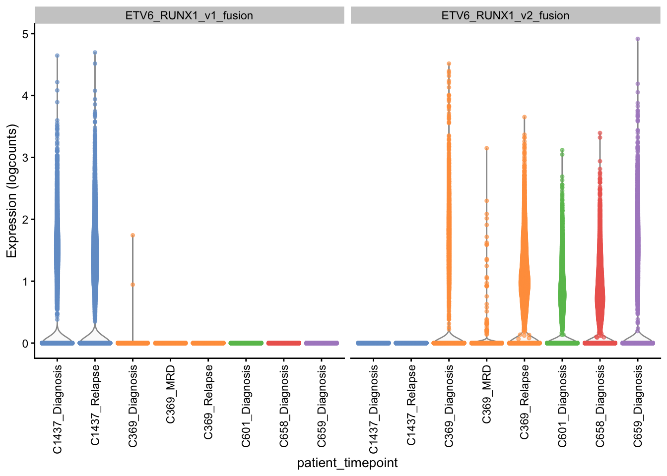
Quality control
Cells are filtered based on the percentage of reads mapping to mitochondrial genes, which is a proxy for cell damage or stress. Sample-specific outlier thresholds are defined using 3 median absolute deviations (MADs) above the median, applied independently per sample to account for differences in cell composition across patients and timepoints.
Identify mitochondrial genes.
rowData(sce)$is_mito <- str_detect(rowData(sce)$Symbol, "^MT-")Calculate per cell quality control metrics.
sce <- addPerCellQC(sce,
                    subsets = list(is_mito = rowData(sce)$is_mito))
Per cell QC
p1 <- plotColData(
  sce,
  "sum",
  x = "patient_timepoint",
  colour_by = "PPID",
  point_size = 0.5) +
  scale_y_log10() +
  annotation_logticks(
    sides = "l",
    short = unit(0.03, "cm"),
    mid = unit(0.06, "cm"),
    long = unit(0.09, "cm"))

p2 <- plotColData(
  sce,
  "detected",
  x = "patient_timepoint",
  colour_by = "PPID",
  point_size = 0.5)

p3 <- plotColData(
  sce,
  "subsets_is_mito_percent",
  x = "patient_timepoint",
  colour_by = "PPID",
  point_size = 0.5)

# Define axis rotation theme
axis_theme <- theme(
  axis.text.x = element_text(angle = 90, hjust = 1, vjust = 0)
)

# Apply axis theme to each plot
p1 <- p1 + axis_theme
p2 <- p2 + axis_theme
p3 <- p3 + axis_theme  # add p3 if you have three plots

# Combine plots with patchwork, collect legends, and set legend at the bottom
combined <- p1 + p2 + p3 +
  plot_layout(guides = "collect", ncol = 2) +
  plot_annotation(
    theme = theme(
      legend.position = "bottom"
    )
  )

# Display combined patchwork
combined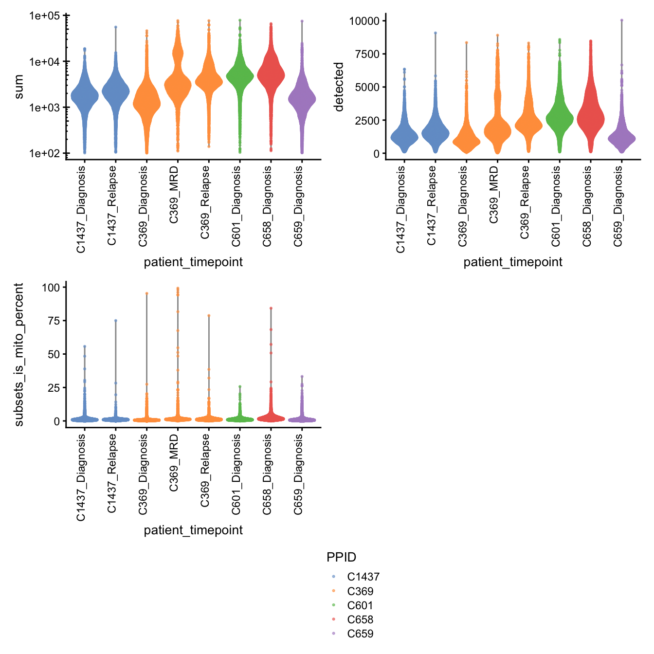
Library size by fusion detection
Fusion-positive cells carry higher total UMI counts than
fusion-negative cells, an effect preserved across both captures
regardless of sequencing depth. A quick exploratory check is shown
below; the publication-quality version (faceted by capture) is now built
as panel D of Supplementary Figure 4, assembled in
B-ALL_exp2_annotate_with_BoneMarrowMap.Rmd, since that
notebook carries this same sum/fusion_detected
information forward on the final annotated object.
sce$fusion_detected <- colSums(counts(sce)[grepl("fusion", rownames(sce)),]) > 0

colData(sce) %>%
  data.frame %>%
  dplyr::select(sum, fusion_detected) %>%
  ggplot(aes(x = fusion_detected, y = sum,
             fill = fusion_detected)) +
  geom_violin() +
  scale_y_log10() -> p1

colData(sce) %>%
  data.frame %>%
  dplyr::select(sum, fusion_detected) %>%
  ggplot(aes(x = fusion_detected, y = sum,
             fill = fusion_detected)) +
  geom_boxplot() +
  scale_y_log10() -> p2

(p1 | p2) + plot_layout(guides = "collect")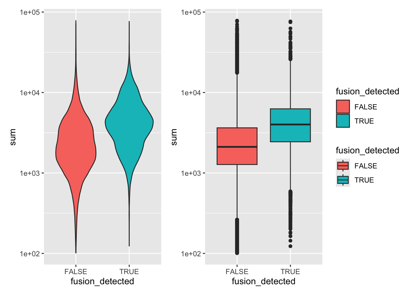
Identify outliers by mitochondrial read %
Filtering on the mitochondrial proportion can identify
stressed/damaged cells and so we seek to identify droplets with
unusually large mitochondrial proportions (i.e. outliers). Outlier
thresholds are defined based on the median absolute deviation (MADs)
from the median value of the metric across all cells. Here, we opt to
use sample-specific thresholds to account for
sample-specific differences.
sce$Sample <- factor(sce$Sample)
sce$patient_timepoint <- factor(sce$patient_timepoint)

mito_drop <- isOutlier(
  metric = sce$subsets_is_mito_percent,
  nmads = 3,
  type = "higher",
  batch = sce$patient_timepoint)
mito_drop_df <- data.frame(
  sample    = colnames(attributes(mito_drop)$thresholds),
  threshold = attributes(mito_drop)$thresholds["higher", ],
  row.names = NULL)
The following table summarises the QC cutoffs:
mito_drop_df %>%
knitr::kable(row.names = FALSE)| sample | threshold |
|---|---|
| C1437_Diagnosis | 3.473106 |
| C1437_Relapse | 2.534330 |
| C369_Diagnosis | 1.921320 |
| C369_MRD | 3.249544 |
| C369_Relapse | 3.548606 |
| C601_Diagnosis | 3.302126 |
| C658_Diagnosis | 6.010868 |
| C659_Diagnosis | 3.074545 |
The majority of cells are retained for all samples.
data.frame(drop = mito_drop,
           sample = sce$patient_timepoint) %>%
  group_by(sample) %>%
  summarise(Drop    = sum(drop),
            Keep    = n() - sum(drop),
            PctKeep = round((n() - sum(drop)) / n() * 100, 1)) %>%
knitr::kable(row.names = FALSE)| sample | Drop | Keep | PctKeep |
|---|---|---|---|
| C1437_Diagnosis | 698 | 11896 | 94.5 |
| C1437_Relapse | 271 | 15653 | 98.3 |
| C369_Diagnosis | 1487 | 13802 | 90.3 |
| C369_MRD | 194 | 2070 | 91.4 |
| C369_Relapse | 509 | 15153 | 96.8 |
| C601_Diagnosis | 661 | 13707 | 95.4 |
| C658_Diagnosis | 598 | 13664 | 95.8 |
| C659_Diagnosis | 1099 | 15088 | 93.2 |
Tag cells that will be dropped.
sce$mito_keep <- !mito_dropIdentify outliers by genes detected (lower bound)
Cells with very few genes detected relative to their peers may
represent empty droplets that passed emptyDrops or highly
degraded cells. A lower-bound outlier threshold is defined per sample
using 3 MADs below the median on the log scale.
gene_drop <- isOutlier(
  metric = sce$detected,
  nmads = 3,
  type = "lower",
  log = TRUE,
  batch = sce$patient_timepoint)

gene_drop_df <- data.frame(
  sample    = colnames(attributes(gene_drop)$thresholds),
  threshold = attributes(gene_drop)$thresholds["lower", ],
  row.names = NULL)

gene_drop_df %>% knitr::kable(row.names = FALSE)| sample | threshold |
|---|---|
| C1437_Diagnosis | 373.1397 |
| C1437_Relapse | 484.8972 |
| C369_Diagnosis | 206.4441 |
| C369_MRD | 423.8947 |
| C369_Relapse | 829.9736 |
| C601_Diagnosis | 1077.5758 |
| C658_Diagnosis | 866.9078 |
| C659_Diagnosis | 309.9088 |
data.frame(drop = gene_drop, sample = sce$patient_timepoint) %>%
  group_by(sample) %>%
  summarise(Drop    = sum(drop),
            Keep    = n() - sum(drop),
            PctKeep = round((n() - sum(drop)) / n() * 100, 1)) %>%
knitr::kable(row.names = FALSE)| sample | Drop | Keep | PctKeep |
|---|---|---|---|
| C1437_Diagnosis | 333 | 12261 | 97.4 |
| C1437_Relapse | 400 | 15524 | 97.5 |
| C369_Diagnosis | 231 | 15058 | 98.5 |
| C369_MRD | 68 | 2196 | 97.0 |
| C369_Relapse | 319 | 15343 | 98.0 |
| C601_Diagnosis | 419 | 13949 | 97.1 |
| C658_Diagnosis | 313 | 13949 | 97.8 |
| C659_Diagnosis | 353 | 15834 | 97.8 |
sce$gene_keep <- !gene_dropCombined filter summary
sce$keep_all <- sce$mito_keep & sce$gene_keep

colData(sce) %>%
  data.frame() %>%
  group_by(patient_timepoint) %>%
  summarise(
    N_total   = n(),
    Drop_mito = sum(!mito_keep),
    Drop_genes = sum(!gene_keep),
    Drop_any  = sum(!keep_all),
    PctKeep   = round(sum(keep_all) / n() * 100, 1)
  ) %>%
  knitr::kable(caption = "Cells removed by each filter and combined",
row.names = FALSE)| patient_timepoint | N_total | Drop_mito | Drop_genes | Drop_any | PctKeep |
|---|---|---|---|---|---|
| C1437_Diagnosis | 12594 | 698 | 333 | 931 | 92.6 |
| C1437_Relapse | 15924 | 271 | 400 | 613 | 96.2 |
| C369_Diagnosis | 15289 | 1487 | 231 | 1589 | 89.6 |
| C369_MRD | 2264 | 194 | 68 | 226 | 90.0 |
| C369_Relapse | 15662 | 509 | 319 | 764 | 95.1 |
| C601_Diagnosis | 14368 | 661 | 419 | 995 | 93.1 |
| C658_Diagnosis | 14262 | 598 | 313 | 822 | 94.2 |
| C659_Diagnosis | 16187 | 1099 | 353 | 1328 | 91.8 |
Scatter plot of total UMI vs. genes detected coloured by filter outcome, to visually confirm thresholds are sensible.
colData(sce) %>%
  data.frame() %>%
  mutate(
    filter_result = case_when(
      !mito_keep ~ "High mito",
      !gene_keep ~ "Low genes",
      TRUE       ~ "Keep"
    ),
    filter_result = factor(filter_result,
                           levels = c("Keep", "High mito", "Low genes"))
  ) %>%
  ggplot(aes(x = sum, y = detected,
             colour = filter_result, alpha = filter_result)) +
  geom_point(size = 0.3) +
  scale_x_log10(labels = scales::comma) +
  scale_y_log10(labels = scales::comma) +
  scale_colour_manual(values = c("Keep"      = "grey70",
                                 "High mito" = "#E41A1C",
                                 "Low genes" = "#377EB8")) +
  scale_alpha_manual(values  = c("Keep"      = 0.2,
                                 "High mito" = 0.8,
                                 "Low genes" = 0.8)) +
  facet_wrap(~ patient_timepoint, ncol = 2) +
  labs(x = "Total UMI (log scale)", y = "Genes detected (log scale)",
       colour = "Filter", alpha = "Filter") +
  theme_classic(base_size = 9) +
  guides(colour = guide_legend(override.aes = list(size = 2, alpha = 1)))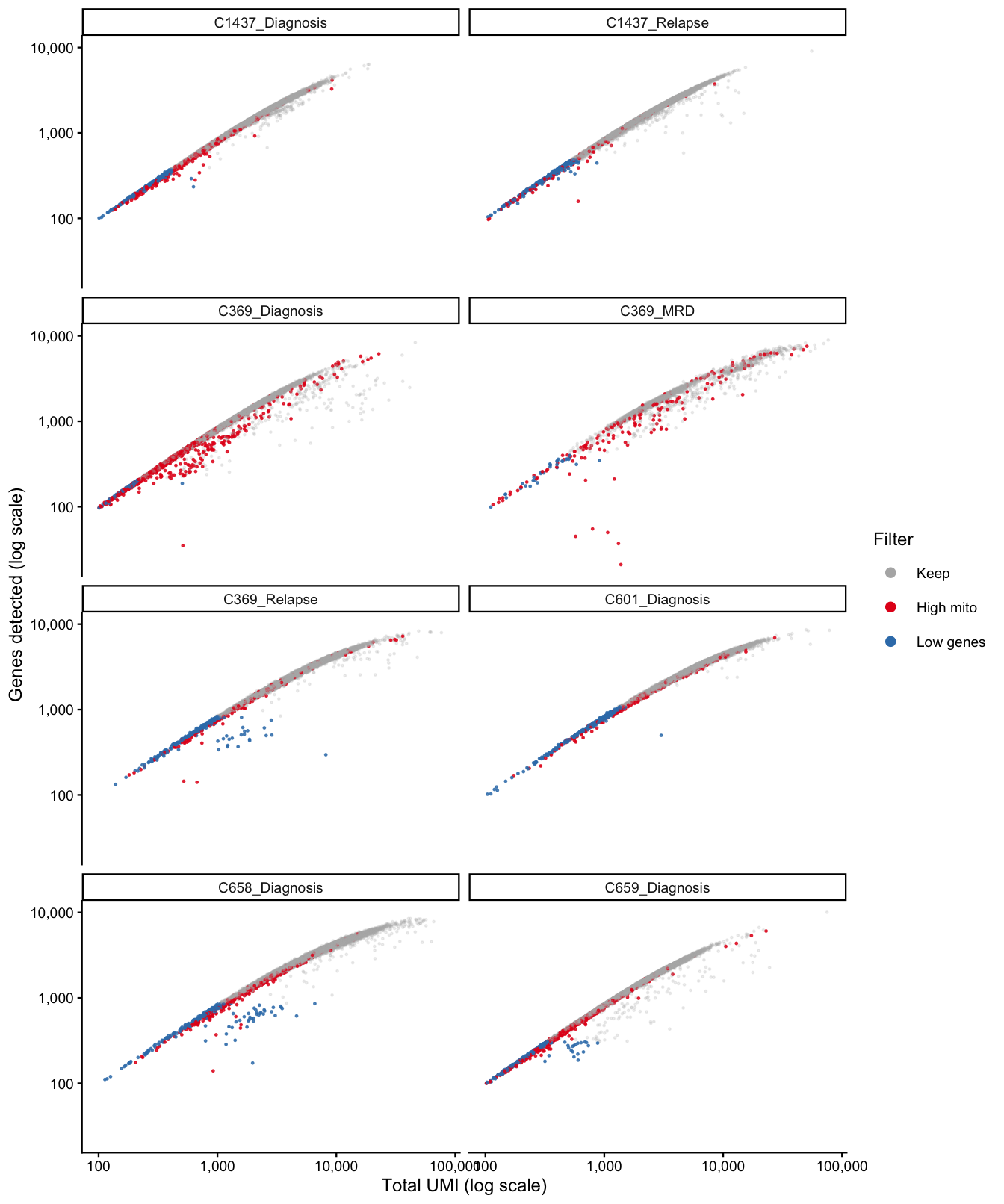
| Version | Author | Date |
|---|---|---|
| d63b2ed | Jovana Maksimovic | 2026-07-15 |
Cells to discard per sample
Another concern is whether the cells removed during QC preferentially derive from particular experimental groups. Reassuringly, the following figure shows that this is not the case.
ggcells(sce) +
  geom_bar(aes(x = patient_timepoint, fill = keep_all)) +
  ylab("Number of droplets") +
  facet_grid(patient_timepoint ~ ., scales = "free_y") +
  theme_bw() +
  theme(axis.text.x = element_text(angle = 90, hjust = 1, vjust = 0))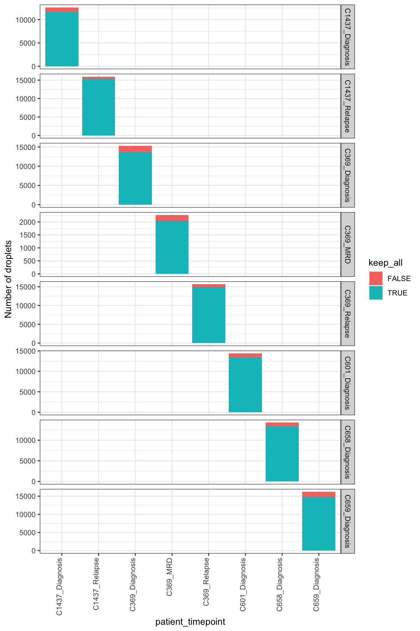
QC metrics of poor vs. good quality cells
This figure compares the QC metrics of discarded and retained droplets.
p1 <- plotColData(
  sce,
  "sum",
  x = "patient_timepoint",
  colour_by = "keep_all",
  point_size = 0.5) +
  scale_y_log10() +
  theme(axis.text.x = element_text(angle = 45, hjust = 1)) +
  annotation_logticks(
    sides = "l",
    short = unit(0.03, "cm"),
    mid = unit(0.06, "cm"),
    long = unit(0.09, "cm"))
p2 <- plotColData(
  sce,
  "detected",
  x = "patient_timepoint",
  colour_by = "keep_all",
  point_size = 0.5) +
  theme(axis.text.x = element_text(angle = 45, hjust = 1))
p3 <- plotColData(
  sce,
  "subsets_is_mito_percent",
  x = "patient_timepoint",
  colour_by = "keep_all",
  point_size = 0.5) +
  theme(axis.text.x = element_text(angle = 45, hjust = 1))

p1 + p2 + p3 + plot_layout(guides = "collect")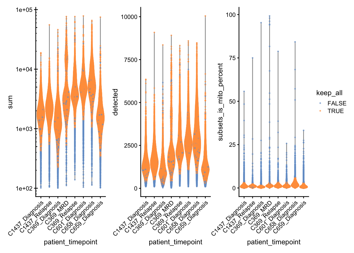
Apply combined filter (mito % + genes detected).
sce_filtered <- sce[, sce$keep_all]
sce_filtered
class: SingleCellExperiment
dim: 37145 99282
metadata(2): Samples Samples
assays(2): counts logcounts
rownames(37145): ENSG00000243485 ENSG00000237613 ...
DEPRECATED_ENSG00000284873 DEPRECATED_ENSG00000285687
rowData names(5): ID Symbol Type is_mito subsets_is_mito
colnames: NULL
colData names(21): Sample Barcode ... gene_keep keep_all
reducedDimNames(0):
mainExpName: NULL
altExpNames(0):Per cell QC after mito % filtering
p1 <- plotColData(
  sce_filtered,
  "sum",
  x = "patient_timepoint",
  colour_by = "PPID",
  point_size = 0.5) +
  scale_y_log10() +
  annotation_logticks(
    sides = "l",
    short = unit(0.03, "cm"),
    mid = unit(0.06, "cm"),
    long = unit(0.09, "cm"))
p2 <- plotColData(
  sce_filtered,
  "detected",
  x = "patient_timepoint",
  colour_by = "PPID",
  point_size = 0.5)
p3 <- plotColData(
  sce_filtered,
  "subsets_is_mito_percent",
  x = "patient_timepoint",
  colour_by = "PPID",
  point_size = 0.5)

# Axis rotation must be applied per-plot
axis_theme <- theme(
  axis.text.x = element_text(angle = 90, hjust = 1, vjust = 0)
)

p1 <- p1 + axis_theme
p2 <- p2 + axis_theme
p3 <- p3 + axis_theme

# Combine with patchwork (no `&`)
combined <- p1 + p2 + p3 +
  plot_layout(guides = "collect", ncol = 2) +
  plot_annotation(
    theme = theme(
      legend.position = "none"
    )
  )

combined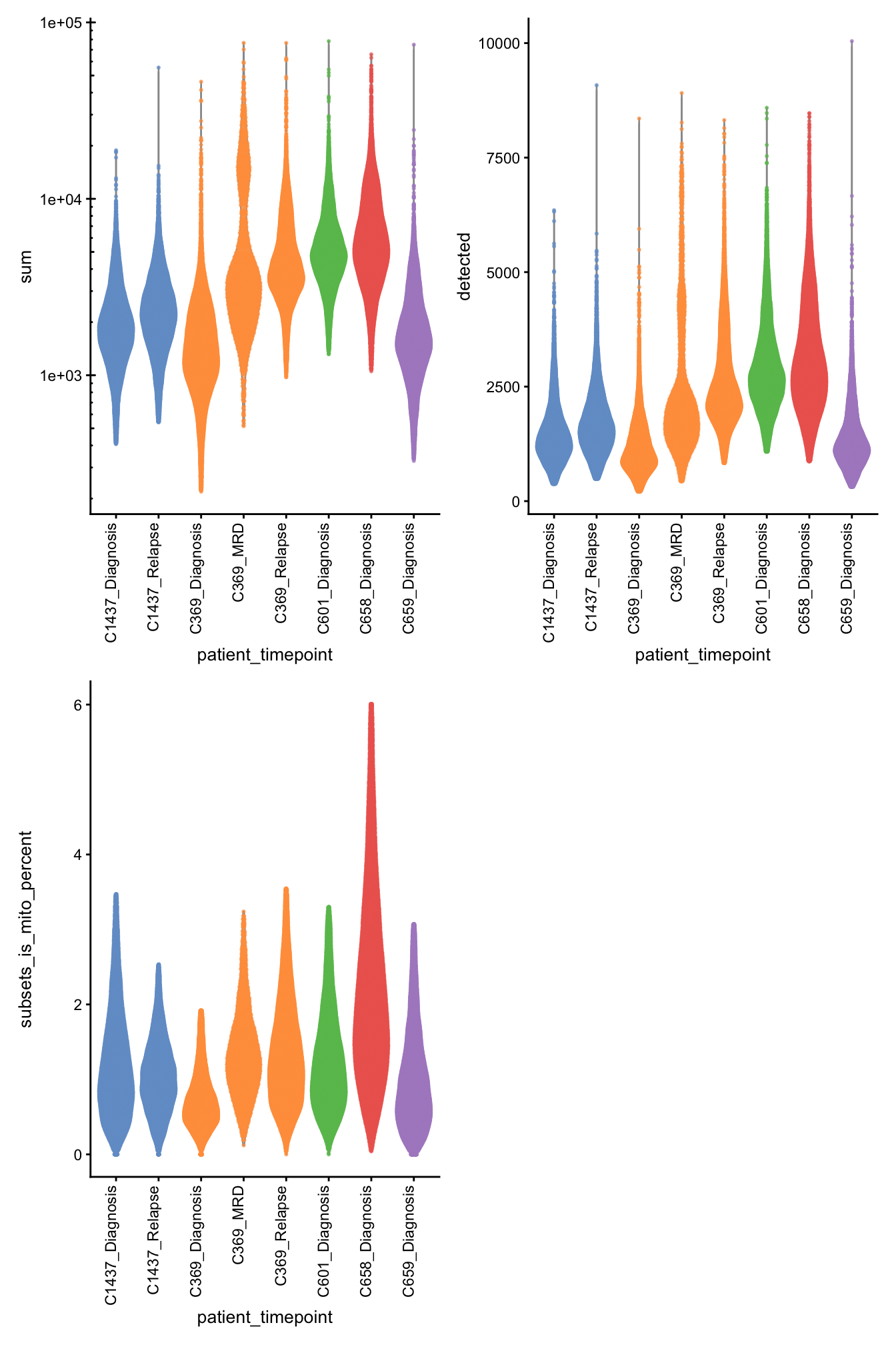
No. non-empty droplets after mito % filtering
p3 <- ggcells(sce_filtered) +
  geom_bar(aes(x = patient_timepoint, fill = PPID)) +
  coord_flip() +
  ylab("Number of droplets") +
  geom_text(stat='count', aes(x = patient_timepoint, label=..count..), hjust=1.5, size=3) +
  guides(fill = "none") +
  theme_bw()

p3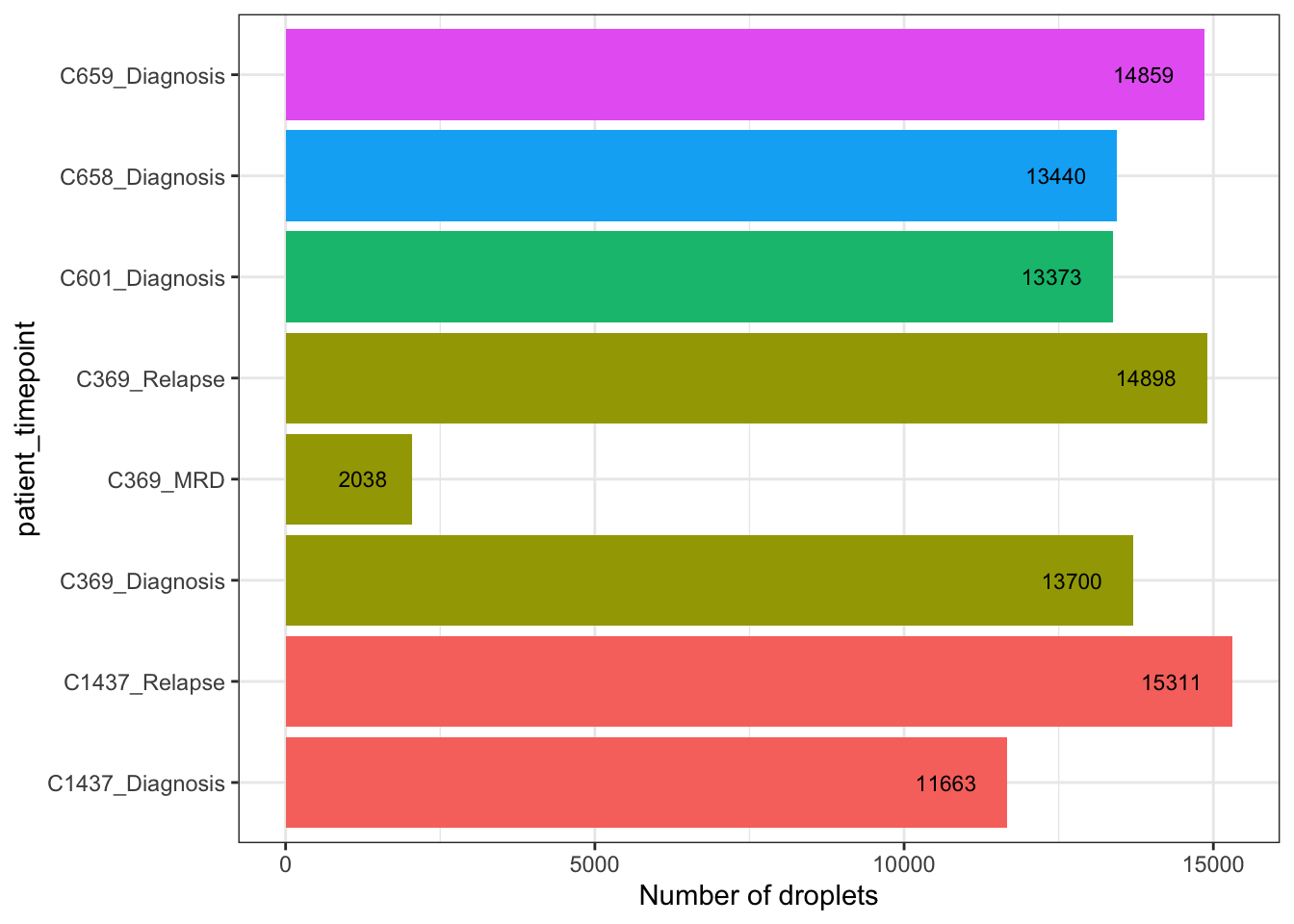
Fusion expression after mito % filtering
plotExpression(sce_filtered,
               rownames(sce_filtered)[fusions],
               x = "patient_timepoint",
               colour_by = "PPID",
               scattermore = TRUE,
               point_size = 1) -> p1

p1 + theme(legend.position = "none",
           axis.text.x = element_text(angle = 90,
                                      hjust = 0.5,
                                      vjust = 1))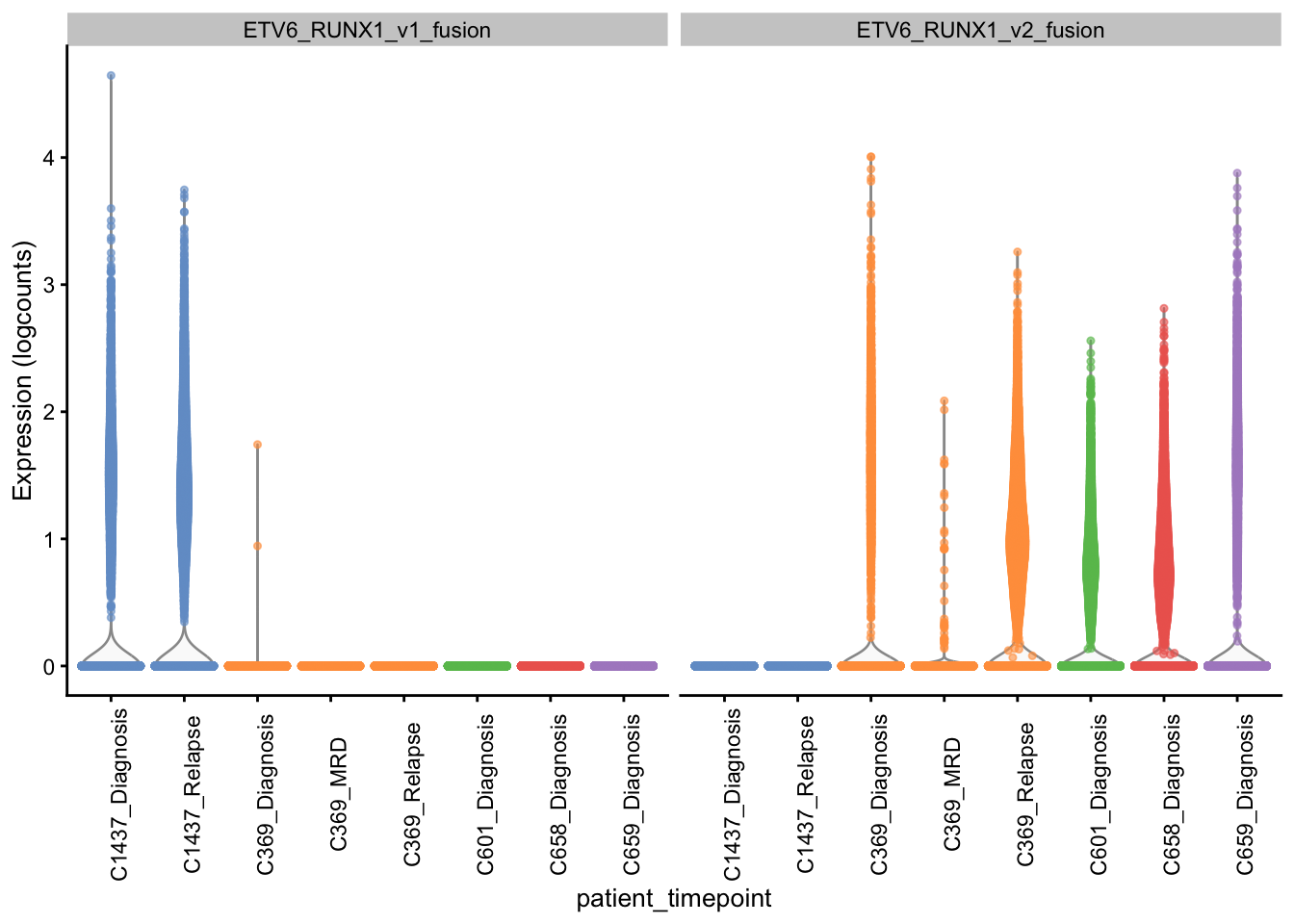
Doublet detection
Doublets (droplets containing two or more cells) are identified using
scDblFinder, which simulates artificial doublets from the
data and scores each cell by its similarity to these simulated profiles.
Cells called as doublets are removed before downstream analysis.
out_doublets <- here("data", "RDS", "exp2_doublets.sce.rds")

if(!file.exists(out_doublets)){
  sce_dbl <- scDblFinder::scDblFinder(sce_filtered,
                                      samples = sce_filtered$Capture,
                                      dbr.sd = 1,
                                      BPPARAM = BiocParallel::MulticoreParam(4))
  saveRDS(sce_dbl, out_doublets)
} else {
  sce_dbl <- readRDS(out_doublets)
}
seu_dbl <- Seurat::CreateSeuratObject(counts = counts(sce_dbl),
meta.data = colData(sce_dbl) %>% data.frame)
seu_dblAn object of class Seurat
37145 features across 99282 samples within 1 assay
Active assay: RNA (37145 features, 0 variable features)
1 layer present: countsUMAP by sample
seu_dbl <- NormalizeData(seu_dbl)
seu_dbl <- FindVariableFeatures(seu_dbl, selection.method = "vst",
                                nfeatures = 3000, verbose = FALSE)
seu_dbl <- ScaleData(seu_dbl)
seu_dbl <- RunPCA(seu_dbl, verbose = FALSE, npcs = 30)
seu_dbl <- RunUMAP(seu_dbl, dims = 1:30, reduction = "pca")
DimPlot(seu_dbl, reduction = "umap", group.by = "patient_timepoint") /
DimPlot(seu_dbl, reduction = "umap", group.by = "scDblFinder.class")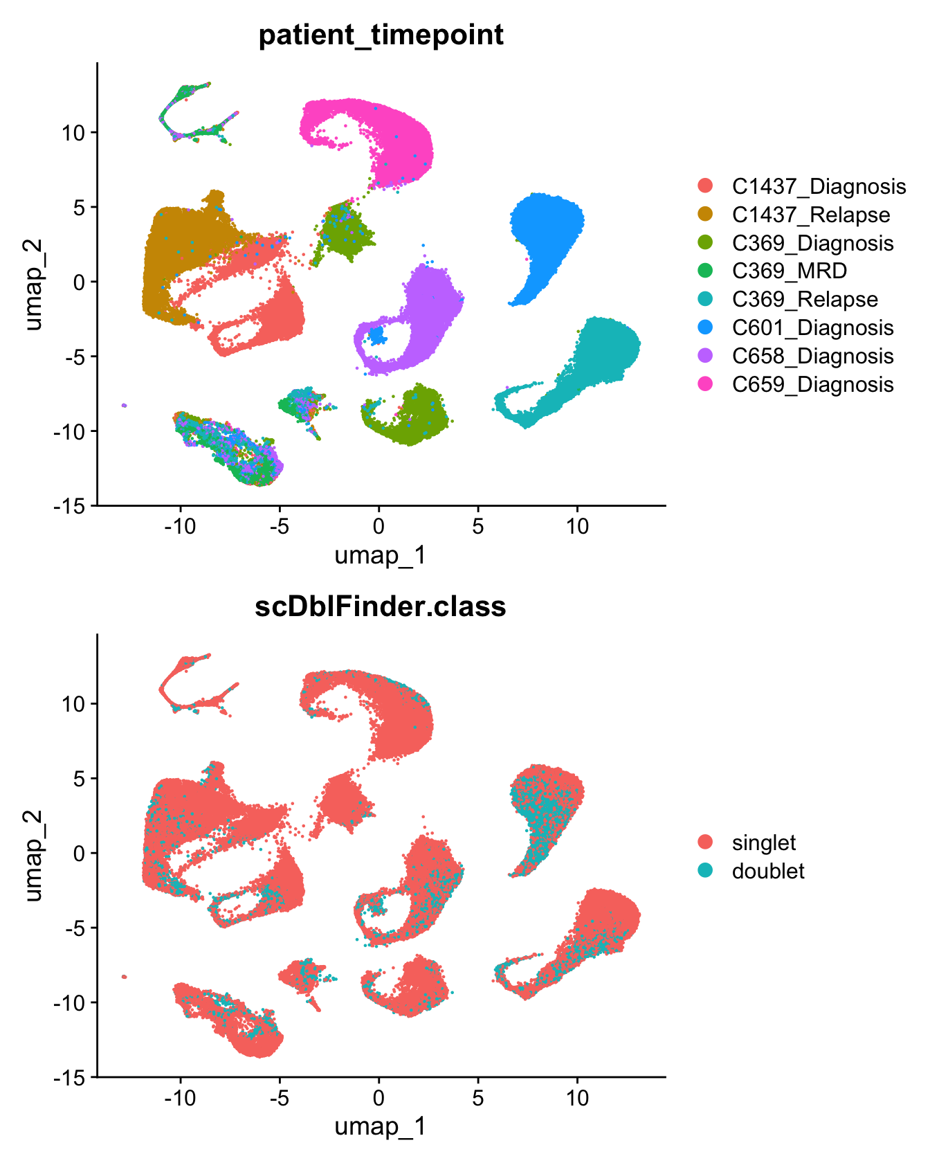
Doublets per sample
seu_dbl@meta.data %>%
  ggplot(aes(x = patient_timepoint, fill = scDblFinder.class)) +
  geom_bar() +
  ylab("Number of droplets") +
  theme_bw() +
  theme(axis.text.x = element_text(angle = 45, hjust = 1)) +
  facet_grid(patient_timepoint ~ ., scales = "free_y")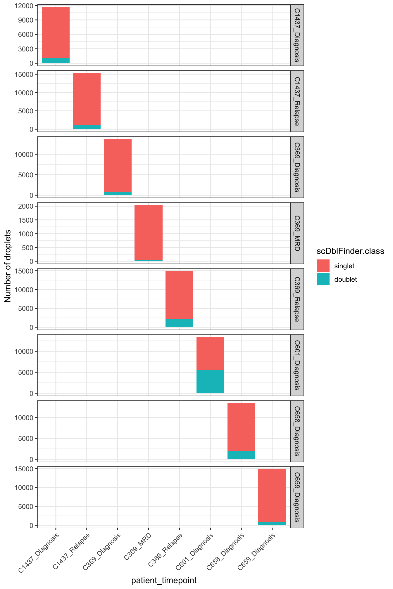
# Check doublet rates per sample
seu_dbl@meta.data %>%
  group_by(patient_timepoint) %>%
  summarise(
    n_total     = n(),
    n_doublet   = sum(scDblFinder.class == "doublet"),
    pct_doublet = round(sum(scDblFinder.class == "doublet") / n() * 100, 1)
  ) %>%
  arrange(desc(pct_doublet))
# A tibble: 8 × 4
patient_timepoint n_total n_doublet pct_doublet
<fct> <int> <int> <dbl>
1 C601_Diagnosis 13373 5560 41.6
2 C369_Relapse 14898 2272 15.3
3 C658_Diagnosis 13440 2006 14.9
4 C1437_Diagnosis 11663 1049 9
5 C1437_Relapse 15311 1217 7.9
6 C369_Diagnosis 13700 754 5.5
7 C659_Diagnosis 14859 806 5.4
8 C369_MRD 2038 37 1.8Filter out doublets.
sce_singlets <- sce_dbl[, sce_dbl$scDblFinder.class != "doublet"]
sce_singlets
class: SingleCellExperiment
dim: 37145 85581
metadata(3): Samples Samples scDblFinder.threshold
assays(2): counts logcounts
rownames(37145): ENSG00000243485 ENSG00000237613 ...
DEPRECATED_ENSG00000284873 DEPRECATED_ENSG00000285687
rowData names(6): ID Symbol ... subsets_is_mito scDblFinder.selected
colnames(85581): cell1 cell2 ... cell99281 cell99282
colData names(25): Sample Barcode ... scDblFinder.weighted
scDblFinder.cxds_score
reducedDimNames(0):
mainExpName: NULL
altExpNames(0):Filter high library size outliers
Even after doublet removal, a small number of cells with extreme total UMI counts remain. These likely represent higher-order multiplets (triplets or greater) that scDblFinder did not flag. Upper-bound outliers are identified per sample at 4 MADs above the median on the log scale.
umi_drop_upper <- isOutlier(
  metric = sce_singlets$sum,
  nmads  = 4,
  type   = "higher",
  log    = TRUE,
  batch  = sce_singlets$patient_timepoint)

data.frame(
  sample    = colnames(attributes(umi_drop_upper)$thresholds),
  threshold = attributes(umi_drop_upper)$thresholds["higher", ],
  row.names = NULL
) %>%
  left_join(
    colData(sce_singlets) %>% data.frame() %>%
      group_by(patient_timepoint) %>%
      summarise(P999 = quantile(sum, 0.999), Max = max(sum)),
    by = c("sample" = "patient_timepoint")
  ) %>%
  knitr::kable(row.names = FALSE,
caption = "Upper UMI thresholds vs P99.9 and Max per sample")| sample | threshold | P999 | Max |
|---|---|---|---|
| C1437_Diagnosis | 9300.179 | 7955.332 | 18352 |
| C1437_Relapse | 11973.530 | 7291.537 | 55491 |
| C369_Diagnosis | 10681.788 | 17105.090 | 41395 |
| C369_MRD | 44695.892 | 59478.000 | 76564 |
| C369_Relapse | 16521.057 | 34908.125 | 76476 |
| C601_Diagnosis | 15207.193 | 29177.048 | 78312 |
| C658_Diagnosis | 40402.461 | 50135.182 | 65878 |
| C659_Diagnosis | 10105.454 | 15658.660 | 74783 |
data.frame(drop = umi_drop_upper, sample = sce_singlets$patient_timepoint) %>%
  group_by(sample) %>%
  summarise(Drop = sum(drop), Keep = n() - sum(drop)) %>%
  knitr::kable(row.names = FALSE,
caption = "Cells removed by upper UMI filter after doublet removal")| sample | Drop | Keep |
|---|---|---|
| C1437_Diagnosis | 5 | 10609 |
| C1437_Relapse | 3 | 14091 |
| C369_Diagnosis | 42 | 12904 |
| C369_MRD | 10 | 1991 |
| C369_Relapse | 104 | 12522 |
| C601_Diagnosis | 87 | 7726 |
| C658_Diagnosis | 28 | 11406 |
| C659_Diagnosis | 22 | 14031 |
sce_qc <- sce_singlets[, !umi_drop_upper]
sce_qc
class: SingleCellExperiment
dim: 37145 85280
metadata(3): Samples Samples scDblFinder.threshold
assays(2): counts logcounts
rownames(37145): ENSG00000243485 ENSG00000237613 ...
DEPRECATED_ENSG00000284873 DEPRECATED_ENSG00000285687
rowData names(6): ID Symbol ... subsets_is_mito scDblFinder.selected
colnames(85280): cell1 cell2 ... cell99281 cell99282
colData names(25): Sample Barcode ... scDblFinder.weighted
scDblFinder.cxds_score
reducedDimNames(0):
mainExpName: NULL
altExpNames(0):Cells retained per sample after filtering (grouped by capture), and
per-sample violin plots of total UMI count, genes detected, and
mitochondrial read percentage, feed directly into Supplementary
Figure 4, assembled below from sce_qc.
Save outputs
out <- here("data", "RDS", "ball_exp2_qc.sce.rds")
if(!file.exists(out)) saveRDS(sce_qc, out)
fs::file_chmod(out, "664")
try(fs::file_chown(out, group_id = "oshlack_lab"),
    silent = TRUE)
Publication figure: Supplementary Figure 4
This section assembles the full Experiment 2 QC / probe-specificity
figure (Supplementary Figure 4) as a single
patchwork, using only sce_qc (saved above).
None of the five panels depend on the BoneMarrowMap annotation performed
in B-ALL_exp2_annotate_with_BoneMarrowMap.Rmd — panels A/B
use QC metrics already in sce_qc’s colData,
panel C uses the raw fusion probe counts, and panels D/E need
patient_fusion (recomputed here) and cell cycle phase
(Seurat::CellCycleScoring()). A single lightweight Seurat
wrapper (seu_fig4) is built once, from a
gene-ID-to-symbol-converted copy of sce_qc (same conversion
as B-ALL_exp2_annotate_with_BoneMarrowMap.Rmd’s
deduplicate-gene-ids chunk, needed so
CellCycleScoring() can match
cc.genes$s.genes/g2m.genes by symbol) — the
two custom fusion probe features carry the same string as both their ID
and their Symbol
(ETV6-RUNX1-v1-fusion/v2-fusion), confirmed by
the annotate notebook itself looking them up successfully immediately
after that same conversion, so one object serves both the fusion-probe
lookups and the cell cycle scoring; there’s no need for a second,
separately-named copy. It plays no other role in the notebook and is not
saved. Panel A shows cells retained per sample after QC, grouped by
capture. Panel B shows per-sample violin plots of total UMI count, genes
detected, and mitochondrial percentage. Panel C shows probe binding
specificity (correct vs. cross-probe detection). Panel D shows fusion
detection rate (% cells fusion-positive) by cell cycle phase, faceted by
capture. Panel E shows library size by cell cycle phase, faceted by
capture.
## Gene ID -> Symbol conversion (same as B-ALL_exp2_annotate_with_BoneMarrowMap.Rmd's
## deduplicate-gene-ids chunk) is done once, up front, so the single seu_fig4
## object built from it works for everything below: CellCycleScoring() (needs
## gene symbols) and the fusion-probe lookups (the two custom probe rows keep
## their "ETV6-RUNX1-v1/v2-fusion" identifiers through this conversion, since
## Symbol == ID for those rows).
sce_symbols <- sce_qc
rownames(sce_symbols) <- rowData(sce_symbols)$Symbol
dup_symbols <- rownames(sce_symbols)[duplicated(rownames(sce_symbols))]
rownames(sce_symbols) <- ifelse(
  rownames(sce_symbols) %in% dup_symbols,
  paste0(rownames(sce_symbols), "_", rowData(sce_symbols)$ID),
  rownames(sce_symbols)
)

seu_fig4 <- CreateSeuratObject(counts = counts(sce_symbols),
                               meta.data = colData(sce_symbols) %>% data.frame)

v1_counts <- GetAssayData(seu_fig4, assay = "RNA", layer = "counts")["ETV6-RUNX1-v1-fusion", ]
v2_counts <- GetAssayData(seu_fig4, assay = "RNA", layer = "counts")["ETV6-RUNX1-v2-fusion", ]

# unname(): GetAssayData()-derived vectors carry cell-barcode names, and
# Seurat's `$<-` will try (and fail) to align by name rather than position
# unless stripped first — see the same note in supp-fig4-panelD.
seu_fig4$patient_fusion <- unname(ifelse(
  v1_counts > 0, "ETV6-RUNX1-v1-fusion",
  ifelse(v2_counts > 0, "ETV6-RUNX1-v2-fusion", "not-detected")
))
# ── Shared palette / capture lookup tables, reused across panels A–E ──────────
sample_colours <- c(
# Capture 1
"C1437_Diagnosis" = "#E41A1C",
"C1437_Relapse" = "#FF7F00",
"C369_Diagnosis" = "#999900",
"C659_Diagnosis" = "#FF69B4",
# Capture 2
"C369_MRD" = "#4DAF4A",
"C369_Relapse" = "#377EB8",
"C601_Diagnosis" = "#984EA3",
"C658_Diagnosis" = "#00CED1"
)
capture_levels_short <- c("Capture 1", "Capture 2")
# Two-line version (bracketed read-depth text on its own line below
# "Capture 1"/"Capture 2") -- used by panels D and E's facet strips.
capture_levels_long <- c("Capture 1\n(4,085 reads/cell)",
"Capture 2\n(22,877 reads/cell)")
# One-line version -- used only by panel B's top violin strip.
capture_levels_long_b <- c("Capture 1 (4,085 reads/cell)",
"Capture 2 (22,877 reads/cell)")
capture_map_short <- c(
"C1437_Diagnosis" = "Capture 1",
"C1437_Relapse" = "Capture 1",
"C369_Diagnosis" = "Capture 1",
"C659_Diagnosis" = "Capture 1",
"C369_Relapse" = "Capture 2",
"C369_MRD" = "Capture 2",
"C601_Diagnosis" = "Capture 2",
"C658_Diagnosis" = "Capture 2"
)
capture_map_long <- c(
"C1437_Diagnosis" = "Capture 1\n(4,085 reads/cell)",
"C1437_Relapse" = "Capture 1\n(4,085 reads/cell)",
"C369_Diagnosis" = "Capture 1\n(4,085 reads/cell)",
"C659_Diagnosis" = "Capture 1\n(4,085 reads/cell)",
"C369_Relapse" = "Capture 2\n(22,877 reads/cell)",
"C369_MRD" = "Capture 2\n(22,877 reads/cell)",
"C601_Diagnosis" = "Capture 2\n(22,877 reads/cell)",
"C658_Diagnosis" = "Capture 2\n(22,877 reads/cell)"
)
capture_map_long_b <- c(
"C1437_Diagnosis" = "Capture 1 (4,085 reads/cell)",
"C1437_Relapse" = "Capture 1 (4,085 reads/cell)",
"C369_Diagnosis" = "Capture 1 (4,085 reads/cell)",
"C659_Diagnosis" = "Capture 1 (4,085 reads/cell)",
"C369_Relapse" = "Capture 2 (22,877 reads/cell)",
"C369_MRD" = "Capture 2 (22,877 reads/cell)",
"C601_Diagnosis" = "Capture 2 (22,877 reads/cell)",
"C658_Diagnosis" = "Capture 2 (22,877 reads/cell)"
)
# v1-probe samples: C1437 only. All other samples were assigned the v2 probe.
v1_probe_samples <- c("C1437_Diagnosis", "C1437_Relapse")
# Abbreviated display labels (Diagnosis -> Dx, Relapse -> Rel) used only for
# axis text via scale_x_discrete(labels = ...); the underlying patient_timepoint
# values (used for joins against sample_colours/capture_map_*/v1_probe_samples)
# are left unchanged.
sample_labels <- c(
"C1437_Diagnosis" = "C1437_Dx",
"C1437_Relapse" = "C1437_Rel",
"C369_Diagnosis" = "C369_Dx",
"C659_Diagnosis" = "C659_Dx",
"C369_MRD" = "C369_MRD",
"C369_Relapse" = "C369_Rel",
"C601_Diagnosis" = "C601_Dx",
"C658_Diagnosis" = "C658_Dx"
)Panel A: Cell recovery
cell_counts <- data.frame(table(seu_fig4$patient_timepoint)) %>%
  setNames(c("patient_timepoint", "n_cells")) %>%
  mutate(
    patient_timepoint = factor(patient_timepoint,
                               levels = rev(names(sample_colours))),
    Capture = factor(capture_map_short[as.character(patient_timepoint)],
                     levels = capture_levels_short)
  )

pA <- ggplot(cell_counts,
             aes(x = patient_timepoint, y = n_cells,
                 fill = patient_timepoint)) +
  geom_col(width = 0.7) +
  geom_text(aes(label = n_cells),
            hjust = -0.1, size = 2.8, color = "grey30") +
  scale_fill_manual(values = sample_colours, guide = "none") +
  scale_x_discrete(labels = sample_labels) +
  scale_y_continuous(expand = expansion(mult = c(0, 0.15)),
                     labels = scales::comma) +
  coord_flip() +
  facet_grid(Capture ~ ., scales = "free_y", space = "free_y") +
  labs(x = NULL, y = "Cells retained",
       title = "Cell recovery after QC") +
  theme_classic(base_size = 10) +
  theme(
    plot.title         = element_text(size = 10, face = "bold",
                                      color = "grey15", margin = margin(b = 8)),
    axis.text          = element_text(size = 8, color = "grey20"),
    axis.line          = element_line(color = "grey60", linewidth = 0.4),
    axis.ticks         = element_line(color = "grey60", linewidth = 0.3),
    panel.grid.major.x = element_line(color = "grey95", linewidth = 0.4),
    strip.text         = element_text(size = 8, face = "bold", color = "grey15"),
    strip.background   = element_blank()
  )

pA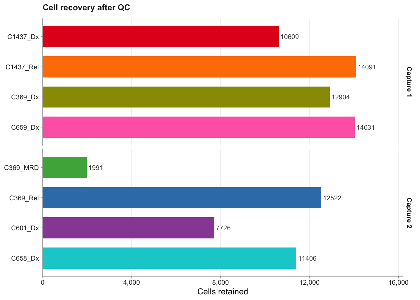
Panel B: QC metric violins
qc_df <- seu_fig4@meta.data %>%
  dplyr::select(patient_timepoint, sum, detected,
                subsets_is_mito_percent) %>%
  mutate(
    patient_timepoint = factor(patient_timepoint,
                               levels = names(sample_colours)),
    Capture_long  = factor(capture_map_long_b[as.character(patient_timepoint)],
                           levels = capture_levels_long_b),
    Capture_short = factor(capture_map_short[as.character(patient_timepoint)],
                           levels = capture_levels_short)
  )

make_qc_violin <- function(df, y_var, y_lab, log_scale = FALSE,
                           top_plot = FALSE) {
  capture_var <- if (top_plot) "Capture_long" else "Capture_short"

  p <- ggplot(df, aes(x = patient_timepoint,
                      y = .data[[y_var]],
                      fill = patient_timepoint)) +
    geom_violin(scale     = "width",
                trim      = TRUE,
                linewidth = 0.3,
                color     = "grey30",
                alpha     = 0.85) +
    geom_boxplot(width         = 0.12,
                 fill          = "white",
                 color         = "grey30",
                 linewidth     = 0.3,
                 outlier.shape = NA) +
    scale_fill_manual(values = sample_colours, guide = "none") +
    scale_x_discrete(labels = sample_labels) +
    facet_grid(~ .data[[capture_var]], scales = "free_x", space = "free_x") +
    labs(x = NULL, y = y_lab) +
    theme_classic(base_size = 9) +
    theme(
      axis.text.x        = element_text(size = 7, color = "grey20",
                                        angle = 45, hjust = 1),
      axis.text.y        = element_text(size = 7, color = "grey30"),
      axis.title.y       = element_text(size = 8, color = "grey20",
                                        margin = margin(r = 4)),
      axis.line          = element_line(color = "grey60", linewidth = 0.4),
      axis.ticks         = element_line(color = "grey60", linewidth = 0.3),
      panel.grid.major.y = element_line(color = "grey95", linewidth = 0.3),
      strip.text         = element_text(size = 8, face = "bold",
                                        color = "grey15"),
      strip.background   = element_blank()
    )
  if (log_scale) p <- p + scale_y_log10(labels = scales::comma)
  p
}

pB1 <- make_qc_violin(qc_df, "sum", "Total UMI (log scale)",
                      log_scale = TRUE, top_plot = TRUE)
pB2 <- make_qc_violin(qc_df, "detected", "Genes detected") +
  theme(strip.text = element_blank())
pB3 <- make_qc_violin(qc_df, "subsets_is_mito_percent", "Mitochondrial %") +
  theme(strip.text = element_blank())

pA | (pB1 / pB2 / pB3)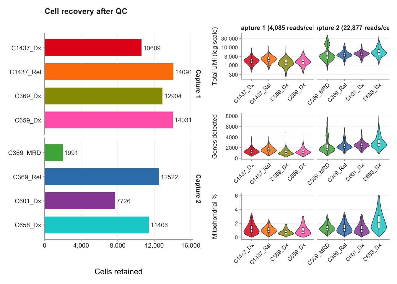
Panel C: Probe binding specificity
Cross-sample probe hybridisation is quantified as the number of cells carrying UMI counts from the probe that does not match their sample’s assigned breakpoint (v1 probe was only ever added to C1437 samples; v2 probe was added to all other samples). Bars are coloured by probe identity (v1 vs. v2), not by a derived correct/incorrect label — so for a v1-probe sample the v1-coloured bar is the real signal and the v2-coloured bar is cross-probe background, and vice versa for a v2-probe sample. Raw cell counts are shown rather than percentages, since the cross-probe counts are at the floor of detection (0 or 1 cell) and are invisible on a percentage scale; a log10(n+1) axis lets both bars be read on the same panel, with exact counts labelled directly.
probe_df <- data.frame(
  patient_timepoint = seu_fig4$patient_timepoint,
  v1_UMI = v1_counts,
  v2_UMI = v2_counts
) %>%
  mutate(
    probe_assigned     = ifelse(patient_timepoint %in% v1_probe_samples,
                                "v1 probe", "v2 probe"),
    incorrect_detected = ifelse(probe_assigned == "v1 probe", v2_UMI > 0, v1_UMI > 0)
  )

cat(glue::glue(
  "Cross-probe (incorrect binding) UMI signal detected in {sum(probe_df$incorrect_detected)} of {nrow(probe_df)} cells profiled ({round(100 * mean(probe_df$incorrect_detected), 4)}%).\n"
))
Cross-probe (incorrect binding) UMI signal detected in 1 of 85280 cells profiled (0.0012%).# Colour by probe identity (v1/v2), not correct/incorrect -- so whichever
# probe was NOT assigned to a sample shows up in that probe's own colour,
# making cross-probe background visually self-evident rather than needing a
# separate "incorrect" category.
probe_summary <- probe_df %>%
group_by(patient_timepoint) %>%
summarise(
n_v1 = sum(v1_UMI > 0),
n_v2 = sum(v2_UMI > 0),
.groups = "drop"
) %>%
tidyr::pivot_longer(cols = c(n_v1, n_v2),
names_to = "probe", values_to = "n") %>%
mutate(
probe = factor(probe, levels = c("n_v1", "n_v2"),
labels = c("ETV6::RUNX1 v1 probe", "ETV6::RUNX1 v2 probe")),
patient_timepoint = factor(patient_timepoint, levels = names(sample_colours)),
Capture = factor(capture_map_short[as.character(patient_timepoint)],
levels = capture_levels_short),
n_plot = n + 1
)
probe_colours <- c(
"ETV6::RUNX1 v1 probe" = "#4E7AC7",
"ETV6::RUNX1 v2 probe" = "#C74E4E"
)
pC <- ggplot(probe_summary, aes(x = patient_timepoint, y = n_plot, fill = probe)) +
geom_col(position = position_dodge(width = 0.8), width = 0.7) +
geom_text(aes(label = scales::comma(n)),
position = position_dodge(width = 0.8),
vjust = -0.3, size = 2.5, color = "grey20") +
scale_fill_manual(values = probe_colours, name = NULL) +
scale_x_discrete(labels = sample_labels) +
scale_y_log10(labels = scales::comma,
expand = expansion(mult = c(0, 0.15))) +
facet_wrap(~ Capture, scales = "free_x") +
labs(x = NULL, y = "Cells with probe UMI > 0\n(log10(n+1) scale)",
title = "Probe binding specificity") +
theme_classic(base_size = 10) +
theme(
plot.title = element_text(size = 10, face = "bold",
color = "grey15", margin = margin(b = 8)),
axis.text.x = element_text(size = 7, angle = 45, hjust = 1, color = "grey20"),
axis.text.y = element_text(size = 8, color = "grey30"),
legend.position = "bottom",
legend.text = element_text(size = 8),
strip.text = element_text(size = 9, face = "bold", color = "grey15"),
strip.background = element_blank()
)
pC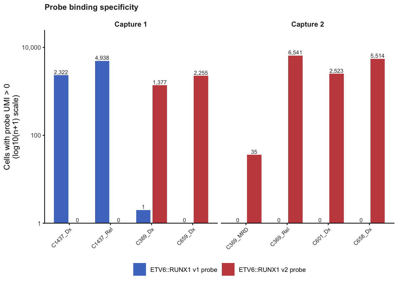
Panel D: Fusion detection rate by cell cycle phase
Cell cycle phase is scored using Seurat’s built-in S/G2M gene sets. Fusion detection is binary per cell, so unlike panel E it isn’t shown as a violin — instead it’s the % of cells fusion-positive per phase, with a chi-squared test of independence (Phase × detection status) annotated per facet, run separately by capture so the phase effect isn’t confounded with the capture-depth effect.
## seu_fig4 already has symbol-based rownames (converted once in
## supp-fig4-setup), so CellCycleScoring() can match cc.genes$s.genes/g2m.genes
## directly -- no need for a second object.
seu_fig4 <- NormalizeData(seu_fig4, verbose = FALSE)
seu_fig4 <- CellCycleScoring(seu_fig4,
                             s.features   = cc.genes$s.genes,
                             g2m.features = cc.genes$g2m.genes)

## factor()/GetAssayData()-derived named vectors can carry cell-barcode names
## that Seurat's `$<-` will try to align by name rather than position; unname()
## forces the safe positional assignment (values are already in column order).
seu_fig4$Capture <- unname(factor(capture_map_long[as.character(seu_fig4$patient_timepoint)],
                                  levels = capture_levels_long))

phase_df <- seu_fig4@meta.data %>%
  filter(!is.na(Phase)) %>%
  mutate(
    Phase           = factor(Phase, levels = c("G1", "S", "G2M")),
    fusion_detected = patient_fusion != "not-detected"
  )

phase_colours <- c("G1" = "#E69F00", "S" = "#009E73", "G2M" = "#56B4E9")

format_pval_sci <- function(p, digits = 2) {
  sci   <- formatC(p, format = "e", digits = digits)
  parts <- strsplit(sci, "e")[[1]]
  sprintf("%s ~ '%s' ~ 10^%d", parts[1], "×", as.integer(parts[2]))
}

phase_fusion_summary <- phase_df %>%
  group_by(Capture, Phase) %>%
  summarise(
    total           = n(),
    fusion_positive = sum(fusion_detected),
    pct_fusion      = round(fusion_positive / total * 100, 1),
    .groups         = "drop"
  ) %>%
  mutate(label = paste0(pct_fusion, "%"))

# Chi-squared test of independence run separately per capture (pooling would
# confound phase with the capture-depth effect), one annotation per facet.
chisq_results <- lapply(split(phase_df, phase_df$Capture), function(df) {
  chisq.test(table(df$Phase, df$fusion_detected))
})

chisq_by_capture <- data.frame(
  Capture = names(chisq_results),
  ## No "Chi-squared test:" prefix -- the chi^2 symbol already says what it
  ## is, so dropping it shortens the label back to one line and gives more
  ## room before hitting the panel edge.
  label   = vapply(names(chisq_results), function(cap) {
    k <- chisq_results[[cap]]
    sprintf("italic(chi)^2 == %.1f ~ ',' ~ italic(p) == %s",
           k$statistic, format_pval_sci(k$p.value))
  }, character(1)),
  y_max   = vapply(names(chisq_results), function(cap) {
    max(phase_fusion_summary$pct_fusion[phase_fusion_summary$Capture == cap])
  }, numeric(1)),
  stringsAsFactors = FALSE
) %>%
  mutate(Capture = factor(Capture, levels = capture_levels_long))

# NOTE: a hard scale_y_continuous(limits = ...) previously capped this axis at
# 48 (fine when captures were pooled at ~20-34%), but split by capture, one
# facet's rate climbed above that — `limits` converts out-of-range values to
# NA rather than clipping the view, so those bars were silently deleted. Using
# a free y-scale and positioning the annotation relative to each facet's own
# max (not a fixed y) avoids the same failure mode recurring.
pD <- ggplot(phase_fusion_summary, aes(x = Phase, y = pct_fusion, fill = Phase)) +
  geom_col(width = 0.5) +
  geom_text(aes(label = label), vjust = -0.5, size = 3.2) +
  geom_text(data = chisq_by_capture,
           aes(x = 0.6, y = y_max * 1.42, label = label),
           inherit.aes = FALSE, parse = TRUE,
           hjust = 0, vjust = 1, size = 2.6, color = "grey30") +
  scale_fill_manual(values = phase_colours, guide = "none") +
  scale_y_continuous(expand = expansion(mult = c(0.02, 0.22))) +
  facet_wrap(~ Capture, scales = "free") +
  labs(x = "Cell cycle phase", y = "% fusion-positive cells",
       title = "Fusion detection by phase") +
  theme_classic(base_size = 10) +
  theme(
    plot.title         = element_text(size = 10, face = "bold", color = "grey15",
                                      margin = margin(b = 8)),
    axis.title         = element_text(size = 9, color = "grey20"),
    axis.text          = element_text(size = 8, color = "grey30"),
    axis.line          = element_line(color = "grey60", linewidth = 0.4),
    axis.ticks         = element_line(color = "grey60", linewidth = 0.3),
    panel.grid.major.y = element_line(color = "grey95", linewidth = 0.4),
    strip.text         = element_text(size = 9, face = "bold", color = "grey15"),
    strip.background   = element_blank()
  )

pD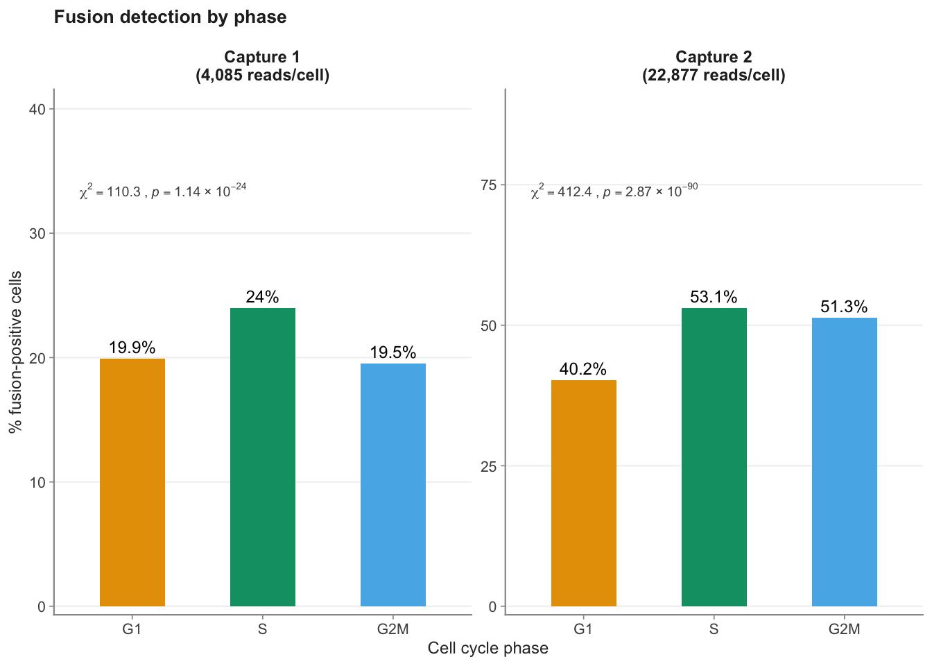
Panel E: Library size by cell cycle phase
Mirrors panel C of Supplementary Figure 1 exactly — a clean
violin/boxplot of library size by phase, no statistical annotation —
faceted here by capture for the same reason as panel D.
scales = "free_y" accommodates the ~5-fold difference in
sequencing depth between captures.
pE <- ggplot(phase_df, aes(x = Phase, y = sum, fill = Phase)) +
  geom_violin(scale = "width", trim = TRUE, linewidth = 0.3,
             color = "grey30", alpha = 0.85) +
  geom_boxplot(width = 0.12, fill = "white", color = "grey30",
              linewidth = 0.4, outlier.shape = NA) +
  scale_fill_manual(values = phase_colours, guide = "none") +
  scale_y_continuous(labels = scales::comma, expand = expansion(mult = c(0.02, 0.08))) +
  facet_wrap(~ Capture, scales = "free_y") +
  labs(x = "Cell cycle phase", y = "Total UMI count",
       title = "Library size by phase") +
  theme_classic(base_size = 10) +
  theme(
    plot.title         = element_text(size = 10, face = "bold", color = "grey15",
                                      margin = margin(b = 8)),
    axis.title         = element_text(size = 9, color = "grey20"),
    axis.text          = element_text(size = 8, color = "grey30"),
    axis.line          = element_line(color = "grey60", linewidth = 0.4),
    axis.ticks         = element_line(color = "grey60", linewidth = 0.3),
    panel.grid.major.y = element_line(color = "grey95", linewidth = 0.4),
    strip.text         = element_text(size = 9, face = "bold", color = "grey15"),
    strip.background   = element_blank()
  )

pE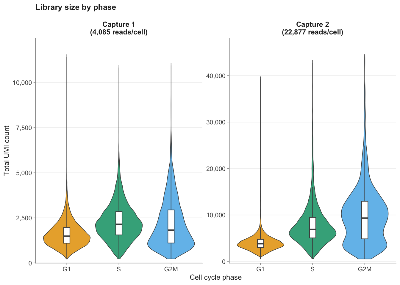
Assemble full patchwork
Tagging follows the same approach as
B-ALL_exp1_clustering.Rmd’s Supplementary Figure 2 assembly
exactly: panel B is itself a nested patchwork (the three stacked
violins), so combining panels with a bare + would expose
each of its leaf ggplots to plot_annotation() and produce
tags A–G instead of A–E. wrap_elements() converts each
conceptual panel — including the nested B stack — into a single opaque
patch first, so patchwork’s automatic tag_levels = "A"
labels exactly five panels. Tag styling (tag_theme) is
applied to the wrap_elements() output, not the pre-wrap
content, since that’s the object patchwork actually themes when placing
the tag.
tag_theme <- theme(plot.tag = element_text(size = 18, face = "bold"))

# Panel B gets its own title (the other panels already have one via labs(title=...))
# so the top row reads as clearly labelled panels rather than one titled + one bare.
supp4_violins <- (pB1 / pB2 / pB3) +
  plot_annotation(title = "QC metrics per sample",
                  theme = theme(plot.title = element_text(
                    size = 10, face = "bold", color = "grey15",
                    margin = margin(b = 8))))

pA_tagged <- wrap_elements(pA) + tag_theme
pB_tagged <- wrap_elements(supp4_violins) + tag_theme
pC_tagged <- wrap_elements(pC) + tag_theme
pD_tagged <- wrap_elements(pD) + tag_theme
pE_tagged <- wrap_elements(pE) + tag_theme

supp4_design <- "
AAABBB
CCDDEE
"

full_patchwork <- pA_tagged + pB_tagged + pC_tagged + pD_tagged + pE_tagged +
  plot_layout(design = supp4_design, heights = c(1.3, 1)) +
  plot_annotation(tag_levels = "A")

full_patchwork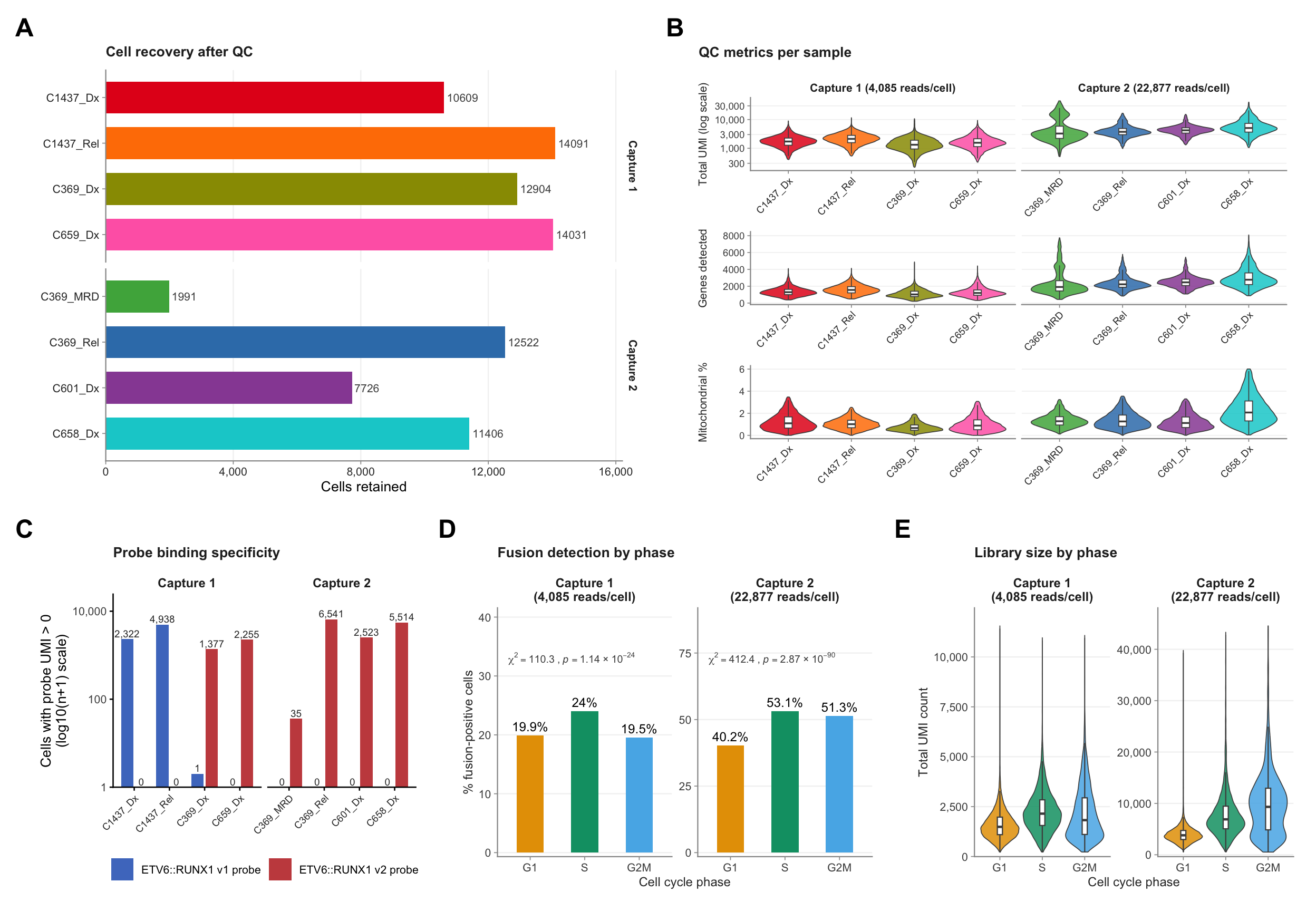
ggsave(here("output", "supp_fig4_exp2_qc_patchwork.pdf"), full_patchwork,
      width = 13, height = 9)
ggsave(here("output", "supp_fig4_exp2_qc_patchwork.png"), full_patchwork,
      width = 13, height = 9, dpi = 300)
Session info
sessioninfo::session_info()─ Session info ───────────────────────────────────────────────────────────────
setting value
version R version 4.4.1 (2024-06-14)
os macOS 15.7.9
system aarch64, darwin20
ui X11
language (EN)
collate en_US.UTF-8
ctype en_US.UTF-8
tz Australia/Melbourne
date 2026-08-25
pandoc 3.8.3 @ /Applications/RStudio.app/Contents/Resources/app/quarto/bin/tools/aarch64/ (via rmarkdown)
quarto 1.9.38 @ /Applications/RStudio.app/Contents/Resources/app/quarto/bin/quarto
─ Packages ───────────────────────────────────────────────────────────────────
! package * version date (UTC) lib source
P abind 1.4-8 2024-09-12 [?] CRAN (R 4.4.1)
P beachmat 2.22.0 2024-11-08 [?] Bioconduc~
P beeswarm 0.4.0 2021-06-01 [?] CRAN (R 4.4.1)
P Biobase * 2.66.0 2024-11-08 [?] Bioconduc~
P BiocGenerics * 0.52.0 2024-11-08 [?] Bioconduc~
P BiocManager 1.30.27 2025-11-14 [?] CRAN (R 4.4.3)
P BiocNeighbors 2.0.1 2024-11-28 [?] Bioconduc~
P BiocParallel 1.40.2 2025-04-08 [?] Bioconductor
P BiocSingular 1.22.0 2024-11-08 [?] Bioconduc~
P bit 4.6.0 2025-03-06 [?] CRAN (R 4.4.1)
P bit64 4.6.0-1 2025-01-16 [?] CRAN (R 4.4.1)
P bslib 0.9.0 2025-01-30 [?] CRAN (R 4.4.1)
P cachem 1.1.0 2024-05-16 [?] CRAN (R 4.4.1)
P callr 3.7.6 2024-03-25 [?] CRAN (R 4.4.0)
P cli 3.6.5 2025-04-23 [?] CRAN (R 4.4.1)
P cluster 2.1.6 2023-12-01 [?] CRAN (R 4.4.1)
P codetools 0.2-20 2024-03-31 [?] CRAN (R 4.4.1)
P colorspace 2.1-1 2024-07-26 [?] CRAN (R 4.4.1)
P cowplot 1.1.3 2024-01-22 [?] CRAN (R 4.4.0)
P crayon 1.5.3 2024-06-20 [?] CRAN (R 4.4.1)
P data.table 1.18.2.1 2026-01-27 [?] CRAN (R 4.4.3)
P DelayedArray 0.32.0 2024-11-08 [?] Bioconduc~
P DelayedMatrixStats 1.28.1 2025-01-09 [?] Bioconduc~
P deldir 2.0-4 2024-02-28 [?] CRAN (R 4.4.1)
P digest 0.6.37 2024-08-19 [?] CRAN (R 4.4.1)
P dotCall64 1.2 2024-10-04 [?] CRAN (R 4.4.1)
P dplyr * 1.1.4 2023-11-17 [?] CRAN (R 4.4.0)
P dqrng 0.4.1 2024-05-28 [?] CRAN (R 4.4.0)
P DropletUtils * 1.26.0 2024-11-08 [?] Bioconduc~
P edgeR 4.4.2 2025-01-27 [?] Bioconduc~
P evaluate 1.0.3 2025-01-10 [?] CRAN (R 4.4.1)
P farver 2.1.2 2024-05-13 [?] CRAN (R 4.4.1)
P fastDummies 1.7.5 2025-01-20 [?] CRAN (R 4.4.1)
P fastmap 1.2.0 2024-05-15 [?] CRAN (R 4.4.1)
P fitdistrplus 1.2-2 2025-01-07 [?] CRAN (R 4.4.1)
P forcats * 1.0.0 2023-01-29 [?] CRAN (R 4.4.0)
P fs 1.6.6 2025-04-12 [?] CRAN (R 4.4.1)
P future 1.49.0 2025-05-09 [?] CRAN (R 4.4.1)
P future.apply 1.11.3 2024-10-27 [?] CRAN (R 4.4.1)
P generics 0.1.4 2025-05-09 [?] CRAN (R 4.4.1)
P GenomeInfoDb * 1.42.3 2025-01-27 [?] Bioconduc~
P GenomeInfoDbData 1.2.13 2025-05-28 [?] Bioconductor
P GenomicRanges * 1.58.0 2024-11-08 [?] Bioconduc~
P getPass 0.2-4 2023-12-10 [?] CRAN (R 4.4.1)
P ggbeeswarm 0.7.2 2023-04-29 [?] CRAN (R 4.4.0)
P ggplot2 * 4.0.2 2026-02-03 [?] CRAN (R 4.4.3)
P ggrepel 0.9.6 2024-09-07 [?] CRAN (R 4.4.1)
P ggridges 0.5.6 2024-01-23 [?] CRAN (R 4.4.0)
P git2r 0.36.2 2025-03-29 [?] CRAN (R 4.4.1)
P globals 0.18.0 2025-05-08 [?] CRAN (R 4.4.1)
P glue * 1.8.0 2024-09-30 [?] CRAN (R 4.4.1)
P goftest 1.2-3 2021-10-07 [?] CRAN (R 4.4.1)
P gridExtra 2.3 2017-09-09 [?] CRAN (R 4.4.1)
P gtable 0.3.6 2024-10-25 [?] CRAN (R 4.4.1)
P HDF5Array 1.34.0 2024-11-08 [?] Bioconduc~
P here * 1.0.1 2020-12-13 [?] CRAN (R 4.4.1)
P hms 1.1.3 2023-03-21 [?] CRAN (R 4.4.0)
P htmltools 0.5.8.1 2024-04-04 [?] CRAN (R 4.4.1)
P htmlwidgets 1.6.4 2023-12-06 [?] CRAN (R 4.4.0)
P httpuv 1.6.16 2025-04-16 [?] CRAN (R 4.4.1)
P httr 1.4.7 2023-08-15 [?] CRAN (R 4.4.0)
P ica 1.0-3 2022-07-08 [?] CRAN (R 4.4.1)
P igraph 2.1.4 2025-01-23 [?] CRAN (R 4.4.1)
P IRanges * 2.40.1 2024-12-05 [?] Bioconduc~
P irlba 2.3.5.1 2022-10-03 [?] CRAN (R 4.4.0)
P jquerylib 0.1.4 2021-04-26 [?] CRAN (R 4.4.0)
P jsonlite 2.0.0 2025-03-27 [?] CRAN (R 4.4.1)
P KernSmooth 2.23-24 2024-05-17 [?] CRAN (R 4.4.1)
P knitr 1.50 2025-03-16 [?] CRAN (R 4.4.1)
P labeling 0.4.3 2023-08-29 [?] CRAN (R 4.4.1)
P later 1.4.2 2025-04-08 [?] CRAN (R 4.4.1)
P lattice 0.22-6 2024-03-20 [?] CRAN (R 4.4.1)
P lazyeval 0.2.2 2019-03-15 [?] CRAN (R 4.4.1)
P lifecycle 1.0.4 2023-11-07 [?] CRAN (R 4.4.1)
P limma 3.62.2 2025-01-09 [?] Bioconduc~
P listenv 0.9.1 2024-01-29 [?] CRAN (R 4.4.1)
P lmtest 0.9-40 2022-03-21 [?] CRAN (R 4.4.1)
P locfit 1.5-9.12 2025-03-05 [?] CRAN (R 4.4.1)
P lubridate * 1.9.4 2024-12-08 [?] CRAN (R 4.4.1)
P magrittr 2.0.3 2022-03-30 [?] CRAN (R 4.4.1)
P MASS 7.3-60.2 2024-04-26 [?] CRAN (R 4.4.1)
P Matrix 1.7-0 2024-04-26 [?] CRAN (R 4.4.1)
P MatrixGenerics * 1.18.1 2025-01-09 [?] Bioconduc~
P matrixStats * 1.5.0 2025-01-07 [?] CRAN (R 4.4.1)
P mime 0.13 2025-03-17 [?] CRAN (R 4.4.1)
P miniUI 0.1.2 2025-04-17 [?] CRAN (R 4.4.1)
P nlme 3.1-164 2023-11-27 [?] CRAN (R 4.4.1)
P parallelly 1.45.0 2025-06-02 [?] CRAN (R 4.4.1)
P patchwork * 1.3.0 2024-09-16 [?] CRAN (R 4.4.1)
P pbapply 1.7-4 2025-07-20 [?] CRAN (R 4.4.1)
P pillar 1.10.2 2025-04-05 [?] CRAN (R 4.4.1)
P pkgconfig 2.0.3 2019-09-22 [?] CRAN (R 4.4.1)
P plotly 4.10.4 2024-01-13 [?] CRAN (R 4.4.0)
P plyr 1.8.9 2023-10-02 [?] CRAN (R 4.4.1)
P png 0.1-8 2022-11-29 [?] CRAN (R 4.4.1)
P polyclip 1.10-7 2024-07-23 [?] CRAN (R 4.4.1)
P processx 3.8.6 2025-02-21 [?] CRAN (R 4.4.1)
P progressr 0.15.1 2024-11-22 [?] CRAN (R 4.4.1)
P promises 1.3.3 2025-05-29 [?] CRAN (R 4.4.1)
P ps 1.9.1 2025-04-12 [?] CRAN (R 4.4.1)
P purrr * 1.0.4 2025-02-05 [?] CRAN (R 4.4.1)
P R.methodsS3 1.8.2 2022-06-13 [?] CRAN (R 4.4.1)
P R.oo 1.27.1 2025-05-02 [?] CRAN (R 4.4.1)
P R.utils 2.13.0 2025-02-24 [?] CRAN (R 4.4.1)
P R6 2.6.1 2025-02-15 [?] CRAN (R 4.4.1)
P ragg 1.4.0 2025-04-10 [?] CRAN (R 4.4.1)
P RANN 2.6.2 2024-08-25 [?] CRAN (R 4.4.1)
P RColorBrewer 1.1-3 2022-04-03 [?] CRAN (R 4.4.1)
P Rcpp 1.1.1-1.1 2026-04-24 [?] CRAN (R 4.4.1)
P RcppAnnoy 0.0.22 2024-01-23 [?] CRAN (R 4.4.1)
P RcppHNSW 0.6.0 2024-02-04 [?] CRAN (R 4.4.1)
P readr * 2.1.5 2024-01-10 [?] CRAN (R 4.4.0)
renv 1.1.4 2025-03-20 [1] CRAN (R 4.4.1)
P reshape2 1.4.4 2020-04-09 [?] CRAN (R 4.4.0)
P reticulate 1.42.0 2025-03-25 [?] CRAN (R 4.4.1)
P rhdf5 2.50.2 2025-01-09 [?] Bioconduc~
P rhdf5filters 1.18.1 2025-03-06 [?] Bioconduc~
P Rhdf5lib 1.28.0 2024-11-08 [?] Bioconduc~
P rlang 1.1.6 2025-04-11 [?] CRAN (R 4.4.1)
P rmarkdown 2.29 2024-11-04 [?] CRAN (R 4.4.1)
P ROCR 1.0-11 2020-05-02 [?] CRAN (R 4.4.0)
P rprojroot 2.0.4 2023-11-05 [?] CRAN (R 4.4.1)
P RSpectra 0.16-2 2024-07-18 [?] CRAN (R 4.4.0)
P rstudioapi 0.17.1 2024-10-22 [?] CRAN (R 4.4.1)
P rsvd 1.0.5 2021-04-16 [?] CRAN (R 4.4.0)
P Rtsne 0.17 2023-12-07 [?] CRAN (R 4.4.1)
P S4Arrays 1.6.0 2024-11-08 [?] Bioconduc~
P S4Vectors * 0.44.0 2024-11-08 [?] Bioconduc~
P S7 0.2.0 2024-11-07 [?] CRAN (R 4.4.1)
P sass 0.4.10 2025-04-11 [?] CRAN (R 4.4.1)
P ScaledMatrix 1.14.0 2024-11-08 [?] Bioconduc~
P scales * 1.4.0 2025-04-24 [?] CRAN (R 4.4.1)
P scater * 1.34.1 2025-03-03 [?] Bioconduc~
P scattermore 1.2 2023-06-12 [?] CRAN (R 4.4.0)
P sctransform 0.4.2 2025-04-30 [?] CRAN (R 4.4.1)
P scuttle * 1.16.0 2024-11-08 [?] Bioconduc~
P sessioninfo 1.2.3 2025-02-05 [?] CRAN (R 4.4.1)
P Seurat * 5.3.0 2025-04-23 [?] CRAN (R 4.4.1)
P SeuratObject * 5.1.0 2025-04-22 [?] CRAN (R 4.4.1)
P shiny 1.10.0 2024-12-14 [?] CRAN (R 4.4.1)
P SingleCellExperiment * 1.28.1 2024-11-23 [?] Bioconduc~
P sp * 2.2-0 2025-02-01 [?] CRAN (R 4.4.1)
P spam 2.11-1 2025-01-20 [?] CRAN (R 4.4.1)
P SparseArray 1.6.2 2025-02-20 [?] Bioconduc~
P sparseMatrixStats 1.18.0 2024-11-08 [?] Bioconduc~
P spatstat.data 3.1-6 2025-03-17 [?] CRAN (R 4.4.1)
P spatstat.explore 3.4-3 2025-05-21 [?] CRAN (R 4.4.1)
P spatstat.geom 3.4-1 2025-05-20 [?] CRAN (R 4.4.1)
P spatstat.random 3.4-1 2025-05-20 [?] CRAN (R 4.4.1)
P spatstat.sparse 3.1-0 2024-06-21 [?] CRAN (R 4.4.0)
P spatstat.univar 3.1-3 2025-05-08 [?] CRAN (R 4.4.1)
P spatstat.utils 3.1-4 2025-05-15 [?] CRAN (R 4.4.1)
P statmod 1.5.0 2023-01-06 [?] CRAN (R 4.4.1)
P stringi 1.8.7 2025-03-27 [?] CRAN (R 4.4.1)
P stringr * 1.6.0 2025-11-04 [?] CRAN (R 4.4.1)
P SummarizedExperiment * 1.36.0 2024-11-08 [?] Bioconduc~
P survival 3.6-4 2024-04-24 [?] CRAN (R 4.4.1)
P systemfonts 1.2.3 2025-04-30 [?] CRAN (R 4.4.1)
P tensor 1.5 2012-05-05 [?] CRAN (R 4.4.1)
P textshaping 1.0.1 2025-05-01 [?] CRAN (R 4.4.1)
P tibble * 3.2.1 2023-03-20 [?] CRAN (R 4.4.0)
P tidyr * 1.3.1 2024-01-24 [?] CRAN (R 4.4.1)
P tidyselect 1.2.1 2024-03-11 [?] CRAN (R 4.4.0)
P tidyverse * 2.0.0 2023-02-22 [?] CRAN (R 4.4.0)
P timechange 0.3.0 2024-01-18 [?] CRAN (R 4.4.1)
P tzdb 0.5.0 2025-03-15 [?] CRAN (R 4.4.1)
P UCSC.utils 1.2.0 2024-11-08 [?] Bioconduc~
P utf8 1.2.5 2025-05-01 [?] CRAN (R 4.4.1)
P uwot 0.2.3 2025-02-24 [?] CRAN (R 4.4.1)
P vctrs 0.6.5 2023-12-01 [?] CRAN (R 4.4.0)
P vipor 0.4.7 2023-12-18 [?] CRAN (R 4.4.1)
P viridis 0.6.5 2024-01-29 [?] CRAN (R 4.4.0)
P viridisLite 0.4.2 2023-05-02 [?] CRAN (R 4.4.1)
P vroom 1.6.5 2023-12-05 [?] CRAN (R 4.4.0)
P whisker 0.4.1 2022-12-05 [?] CRAN (R 4.4.1)
P withr 3.0.2 2024-10-28 [?] CRAN (R 4.4.1)
P workflowr * 1.7.1 2023-08-23 [?] CRAN (R 4.4.0)
P xfun 0.56 2026-01-18 [?] CRAN (R 4.4.3)
P xtable 1.8-4 2019-04-21 [?] CRAN (R 4.4.1)
P XVector 0.46.0 2024-11-08 [?] Bioconduc~
P yaml 2.3.10 2024-07-26 [?] CRAN (R 4.4.1)
P zlibbioc 1.52.0 2024-11-08 [?] Bioconduc~
P zoo 1.8-14 2025-04-10 [?] CRAN (R 4.4.1)
[1] /Users/maksimovicjovana/projects/active/flex-fusion-probes/renv/library/macos/R-4.4/aarch64-apple-darwin20
[2] /Users/maksimovicjovana/Library/Caches/org.R-project.R/R/renv/sandbox/macos/R-4.4/aarch64-apple-darwin20/f7156815
* ── Packages attached to the search path.
P ── Loaded and on-disk path mismatch.
──────────────────────────────────────────────────────────────────────────────
sessionInfo()R version 4.4.1 (2024-06-14)
Platform: aarch64-apple-darwin20
Running under: macOS 15.7.9
Matrix products: default
BLAS: /Library/Frameworks/R.framework/Versions/4.4-arm64/Resources/lib/libRblas.0.dylib
LAPACK: /Library/Frameworks/R.framework/Versions/4.4-arm64/Resources/lib/libRlapack.dylib; LAPACK version 3.12.0
locale:
[1] en_US.UTF-8/en_US.UTF-8/en_US.UTF-8/C/en_US.UTF-8/en_US.UTF-8
time zone: Australia/Melbourne
tzcode source: internal
attached base packages:
[1] stats4 stats graphics grDevices datasets utils methods
[8] base
other attached packages:
[1] scales_1.4.0 Seurat_5.3.0
[3] SeuratObject_5.1.0 sp_2.2-0
[5] patchwork_1.3.0 scater_1.34.1
[7] scuttle_1.16.0 DropletUtils_1.26.0
[9] SingleCellExperiment_1.28.1 SummarizedExperiment_1.36.0
[11] Biobase_2.66.0 GenomicRanges_1.58.0
[13] GenomeInfoDb_1.42.3 IRanges_2.40.1
[15] S4Vectors_0.44.0 BiocGenerics_0.52.0
[17] MatrixGenerics_1.18.1 matrixStats_1.5.0
[19] glue_1.8.0 here_1.0.1
[21] lubridate_1.9.4 forcats_1.0.0
[23] stringr_1.6.0 dplyr_1.1.4
[25] purrr_1.0.4 readr_2.1.5
[27] tidyr_1.3.1 tibble_3.2.1
[29] ggplot2_4.0.2 tidyverse_2.0.0
[31] workflowr_1.7.1
loaded via a namespace (and not attached):
[1] RcppAnnoy_0.0.22 splines_4.4.1
[3] later_1.4.2 R.oo_1.27.1
[5] polyclip_1.10-7 fastDummies_1.7.5
[7] lifecycle_1.0.4 edgeR_4.4.2
[9] rprojroot_2.0.4 vroom_1.6.5
[11] globals_0.18.0 processx_3.8.6
[13] lattice_0.22-6 MASS_7.3-60.2
[15] magrittr_2.0.3 plotly_4.10.4
[17] limma_3.62.2 sass_0.4.10
[19] rmarkdown_2.29 jquerylib_0.1.4
[21] yaml_2.3.10 httpuv_1.6.16
[23] sctransform_0.4.2 spam_2.11-1
[25] sessioninfo_1.2.3 spatstat.sparse_3.1-0
[27] reticulate_1.42.0 pbapply_1.7-4
[29] cowplot_1.1.3 RColorBrewer_1.1-3
[31] abind_1.4-8 zlibbioc_1.52.0
[33] Rtsne_0.17 R.utils_2.13.0
[35] git2r_0.36.2 GenomeInfoDbData_1.2.13
[37] ggrepel_0.9.6 irlba_2.3.5.1
[39] spatstat.utils_3.1-4 listenv_0.9.1
[41] goftest_1.2-3 RSpectra_0.16-2
[43] spatstat.random_3.4-1 dqrng_0.4.1
[45] fitdistrplus_1.2-2 parallelly_1.45.0
[47] DelayedMatrixStats_1.28.1 codetools_0.2-20
[49] DelayedArray_0.32.0 tidyselect_1.2.1
[51] UCSC.utils_1.2.0 farver_2.1.2
[53] ScaledMatrix_1.14.0 viridis_0.6.5
[55] spatstat.explore_3.4-3 jsonlite_2.0.0
[57] BiocNeighbors_2.0.1 progressr_0.15.1
[59] ggridges_0.5.6 survival_3.6-4
[61] systemfonts_1.2.3 tools_4.4.1
[63] ragg_1.4.0 ica_1.0-3
[65] Rcpp_1.1.1-1.1 gridExtra_2.3
[67] SparseArray_1.6.2 xfun_0.56
[69] HDF5Array_1.34.0 withr_3.0.2
[71] BiocManager_1.30.27 fastmap_1.2.0
[73] rhdf5filters_1.18.1 callr_3.7.6
[75] digest_0.6.37 rsvd_1.0.5
[77] timechange_0.3.0 R6_2.6.1
[79] mime_0.13 textshaping_1.0.1
[81] colorspace_2.1-1 scattermore_1.2
[83] tensor_1.5 spatstat.data_3.1-6
[85] R.methodsS3_1.8.2 utf8_1.2.5
[87] generics_0.1.4 data.table_1.18.2.1
[89] renv_1.1.4 htmlwidgets_1.6.4
[91] httr_1.4.7 S4Arrays_1.6.0
[93] whisker_0.4.1 uwot_0.2.3
[95] pkgconfig_2.0.3 gtable_0.3.6
[97] lmtest_0.9-40 S7_0.2.0
[99] XVector_0.46.0 htmltools_0.5.8.1
[101] dotCall64_1.2 png_0.1-8
[103] spatstat.univar_3.1-3 knitr_1.50
[105] rstudioapi_0.17.1 reshape2_1.4.4
[107] tzdb_0.5.0 nlme_3.1-164
[109] cachem_1.1.0 zoo_1.8-14
[111] rhdf5_2.50.2 KernSmooth_2.23-24
[113] parallel_4.4.1 miniUI_0.1.2
[115] vipor_0.4.7 pillar_1.10.2
[117] grid_4.4.1 vctrs_0.6.5
[119] RANN_2.6.2 promises_1.3.3
[121] BiocSingular_1.22.0 beachmat_2.22.0
[123] xtable_1.8-4 cluster_2.1.6
[125] beeswarm_0.4.0 evaluate_1.0.3
[127] cli_3.6.5 locfit_1.5-9.12
[129] compiler_4.4.1 rlang_1.1.6
[131] crayon_1.5.3 future.apply_1.11.3
[133] labeling_0.4.3 ps_1.9.1
[135] plyr_1.8.9 getPass_0.2-4
[137] fs_1.6.6 ggbeeswarm_0.7.2
[139] stringi_1.8.7 deldir_2.0-4
[141] viridisLite_0.4.2 BiocParallel_1.40.2
[143] lazyeval_0.2.2 spatstat.geom_3.4-1
[145] Matrix_1.7-0 RcppHNSW_0.6.0
[147] hms_1.1.3 bit64_4.6.0-1
[149] sparseMatrixStats_1.18.0 future_1.49.0
[151] Rhdf5lib_1.28.0 statmod_1.5.0
[153] shiny_1.10.0 ROCR_1.0-11
[155] igraph_2.1.4 bslib_0.9.0
[157] bit_4.6.0