MCF7 Experiment 1: Fusion Expression
Normalised fusion expression, per-cell detection, and partner gene comparisons
Jovana Maksimovic
August 25, 2026
Last updated: 2026-08-25
Checks: 7 0
Knit directory: flex-fusion-probes/
This reproducible R Markdown analysis was created with workflowr (version 1.7.1). The Checks tab describes the reproducibility checks that were applied when the results were created. The Past versions tab lists the development history.
Great! Since the R Markdown file has been committed to the Git repository, you know the exact version of the code that produced these results.
Great job! The global environment was empty. Objects defined in the global environment can affect the analysis in your R Markdown file in unknown ways. For reproduciblity it’s best to always run the code in an empty environment.
The command set.seed(20240925) was run prior to running
the code in the R Markdown file. Setting a seed ensures that any results
that rely on randomness, e.g. subsampling or permutations, are
reproducible.
Great job! Recording the operating system, R version, and package versions is critical for reproducibility.
Nice! There were no cached chunks for this analysis, so you can be confident that you successfully produced the results during this run.
Great job! Using relative paths to the files within your workflowr project makes it easier to run your code on other machines.
Great! You are using Git for version control. Tracking code development and connecting the code version to the results is critical for reproducibility.
The results in this page were generated with repository version ada53d3. See the Past versions tab to see a history of the changes made to the R Markdown and HTML files.
Note that you need to be careful to ensure that all relevant files for
the analysis have been committed to Git prior to generating the results
(you can use wflow_publish or
wflow_git_commit). workflowr only checks the R Markdown
file, but you know if there are other scripts or data files that it
depends on. Below is the status of the Git repository when the results
were generated:
Ignored files:
    Ignored:    .DS_Store
    Ignored:    .Rhistory
    Ignored:    .Rproj.user/
    Ignored:    analysis/.gitignore
    Ignored:    analysis/B-ALL_exp2_nonblast_fusion_analysis_cache/
    Ignored:    analysis/obsolete/B-ALL_nonblast_fusion_analysis_cache/
    Ignored:    analysis/projectionFigures/
    Ignored:    code/files/
    Ignored:    data/.DS_Store
    Ignored:    data/BoneMarrowMap/
    Ignored:    data/BoneMarrowMapBoneMarrowMap_SymphonyReference.rds
    Ignored:    data/BoneMarrowMapBoneMarrowMap_uwot_model.uwot
    Ignored:    data/CAPTURE-1-POOL-FLEX/
    Ignored:    data/CAPTURE-2-POOL-FLEX/
    Ignored:    data/Pool-240917-FLEX/
    Ignored:    data/RDS/
    Ignored:    data/Run_1_and_Run_2/
    Ignored:    data/Run_2/
    Ignored:    logs/
    Ignored:    output/
    Ignored:    projectionFigures/
    Ignored:    renv/library/
    Ignored:    renv/staging/

Untracked files:
    Untracked:  CLAUDE.md
    Untracked:  data/Config_Sample_CAPTURE-1-POOL-FLEX.csv
    Untracked:  data/Config_Sample_CAPTURE-2-POOL-FLEX.csv
    Untracked:  data/Config_Sample_Pool-240917-FLEX.csv
    Untracked:  data/analysis_input/ETV6_RUNX1_transcript.csv
    Untracked:  data/cellranger-multi_flex_fusions_pool_1.sbatch
    Untracked:  data/cellranger-multi_flex_fusions_pool_2.sbatch
    Untracked:  data/victoria_stuff/
    Untracked:  methods_updated.md

Unstaged changes:
    Modified:   analysis/B-ALL_exp2_c369_mrd_analysis.Rmd
    Modified:   analysis/B-ALL_exp2_fig4_assembly.Rmd
    Modified:   render_all.sh
Note that any generated files, e.g. HTML, png, CSS, etc., are not included in this status report because it is ok for generated content to have uncommitted changes.
These are the previous versions of the repository in which changes were
made to the R Markdown
(analysis/MCF7_exp1_fusion_expression.Rmd) and HTML
(docs/MCF7_exp1_fusion_expression.html) files. If you’ve
configured a remote Git repository (see ?wflow_git_remote),
click on the hyperlinks in the table below to view the files as they
were in that past version.
| File | Version | Author | Date | Message |
|---|---|---|---|---|
| Rmd | ada53d3 | Jovana Maksimovic | 2026-08-25 | wflow_publish("analysis/MCF7_exp1_fusion_expression.Rmd") |
| html | e69a9f3 | Jovana Maksimovic | 2026-07-15 | Build site. |
| Rmd | b0d8dc3 | Jovana Maksimovic | 2026-07-15 | wflow_publish("analysis/MCF7_exp1_fusion_expression.Rmd") |
| html | 1b5bb97 | Jovana Maksimovic | 2026-05-11 | Build site. |
| Rmd | 1f3159b | Jovana Maksimovic | 2026-05-08 | Rename RDS checkpoints to systematic naming scheme |
| Rmd | 880004a | Jovana Maksimovic | 2026-05-08 | Consolidate MCF7 notebooks: 4 → 3 files; fix absolute paths, remove draft plots, add chunk descriptions |
Load data
Load the MCF7 single-cell experiment (run 1 + run 2 combined) from the post-QC SCE object produced by the quality control notebook.
file <- here("data", "RDS", "exp1_qc.sce.rds")
sce  <- readRDS(file)
Create Seurat object
Gene IDs in the SCE are Ensembl IDs; convert to gene symbols before creating the Seurat object. Duplicate symbols (arising from multiple Ensembl IDs mapping to the same symbol) are disambiguated by appending the Ensembl ID.
rownames(sce) <- rowData(sce)$Symbol
dups          <- rownames(sce)[duplicated(rownames(sce))]
rownames(sce) <- ifelse(
  rownames(sce) %in% dups,
  paste0(rownames(sce), "_", rowData(sce)$ID),
  rownames(sce)
)
table(duplicated(rownames(sce)))
FALSE
37170
Subset to MCF7 cells and create a Seurat object.
seu <- CreateSeuratObject(
  counts    = counts(sce)[, sce$Sample == "MCF7"],
  meta.data = colData(sce[, sce$Sample == "MCF7"]) %>% data.frame()
)
Dimensionality reduction
Normalise, identify highly variable features, scale, and run PCA and UMAP.
out_proc <- here("data", "RDS", "mcf7_processed.seu.rds")

if (!file.exists(out_proc)) {
  seu <- NormalizeData(seu)
  seu <- FindVariableFeatures(seu, selection.method = "vst", nfeatures = 3000, verbose = FALSE)
  seu <- ScaleData(seu)
  seu <- RunPCA(seu, verbose = FALSE, npcs = 30)
  seu <- RunUMAP(seu, dims = 1:30, reduction = "pca")
  saveRDS(seu, out_proc)
} else {
  seu <- readRDS(out_proc)
}
Fusion detection per cell
Per-cell fusion count summary statistics
Identify the set of expressed fusion transcripts (those with at least one count in the dataset) and compute per-cell detection statistics.
mcf7_fusions <- rownames(seu)[str_detect(rownames(seu), "fusion") &
                                rowSums(seu[["RNA"]]$counts) > 0]

fusion_counts    <- seu[["RNA"]]$counts[rownames(seu) %in% mcf7_fusions, ]
fusions_per_cell <- colSums(fusion_counts > 0)

# Summary table of fusions detected per cell
detection_summary <- data.frame(
  n_fusions = as.integer(names(table(fusions_per_cell))),
  n_cells   = as.integer(table(fusions_per_cell)),
  pct_cells = round(as.numeric(prop.table(table(fusions_per_cell))) * 100, 1)
)
detection_summary
n_fusions n_cells pct_cells
1 0 16 0.2
2 1 53 0.7
3 2 114 1.6
4 3 239 3.4
5 4 551 7.7
6 5 910 12.8
7 6 1193 16.7
8 7 1175 16.5
9 8 938 13.2
10 9 765 10.7
11 10 505 7.1
12 11 343 4.8
13 12 181 2.5
14 13 85 1.2
15 14 40 0.6
16 15 15 0.2
17 16 3 0.0
18 17 1 0.0# Aggregate summary statistics
data.frame(
statistic = c(
"Total cells", "Cells with ≥1 fusion", "% cells with ≥1 fusion",
"Mean fusions per cell", "Median fusions per cell", "SD fusions per cell",
"Min fusions per cell", "Max fusions per cell",
"25th percentile", "75th percentile"
),
value = c(
ncol(seu),
sum(fusions_per_cell > 0),
round(mean(fusions_per_cell > 0) * 100, 1),
round(mean(fusions_per_cell), 2),
median(fusions_per_cell),
round(sd(fusions_per_cell), 2),
min(fusions_per_cell),
max(fusions_per_cell),
quantile(fusions_per_cell, 0.25),
quantile(fusions_per_cell, 0.75)
)
) statistic value
1 Total cells 7127.00
2 Cells with ≥1 fusion 7111.00
3 % cells with ≥1 fusion 99.80
4 Mean fusions per cell 7.08
5 Median fusions per cell 7.00
6 SD fusions per cell 2.48
7 Min fusions per cell 0.00
8 Max fusions per cell 17.00
9 25th percentile 5.00
10 75th percentile 9.00Histogram and UMAP coloured by fusion count (Figure 2B, 2C)
Each cell is coloured by the number of fusion transcripts detected. The shared colour palette is used in both the histogram and the UMAP so they can be read together.
# Add per-cell fusion count to Seurat metadata
colSums(fusion_counts > 0) %>%
  as.data.frame() %>%
  rownames_to_column(var = "Cell") %>%
  dplyr::rename("Detected" = ".") -> mcf7_fusions_expressed

seu$n_fusions_detected <- mcf7_fusions_expressed$Detected[
  match(colnames(seu), mcf7_fusions_expressed$Cell)
]

# Shared colour palette: light grey (0 fusions) → black (17 fusions)
fusion_levels  <- sort(unique(seu$n_fusions_detected))
fusion_colours <- setNames(
  c(
    "#DCDCDC", "#999999", "#92C5DE", "#56B4E9", "#0072B2",
    "#B8E186", "#4DAC26", "#009E73", "#7FBC41", "#F0E442",
    "#FDBF6F", "#F4A582", "#E69F00", "#D01C8B", "#CC79A7",
    "#F1B6DA", "#D55E00", "#000000"
  ),
  as.character(0:17)
)
# Histogram: number of cells by fusion count
p_hist <- ggplot(mcf7_fusions_expressed,
aes(x = Detected, fill = as.character(Detected))) +
geom_histogram(binwidth = 1, color = "black", linewidth = 0.3) +
scale_fill_manual(values = fusion_colours, guide = "none") +
scale_x_continuous(breaks = fusion_levels) +
labs(x = "No. fusions detected per cell", y = "No. cells") +
theme_classic()
# Helper: adds UMAP axis arrows and removes default axis elements
umap_axis_theme <- function(plot, label = "UMAP", arrow_len = 0.08, fontsize = 10) {
built <- ggplot_build(plot)
x_range <- built$layout$panel_params[[1]]$x.range
y_range <- built$layout$panel_params[[1]]$y.range
x_span <- diff(x_range)
y_span <- diff(y_range)
ox <- x_range[1] + 0.02 * x_span
oy <- y_range[1] + 0.02 * y_span
ax_end <- ox + arrow_len * x_span
ay_end <- oy + arrow_len * y_span
lx <- ox + (arrow_len / 2) * x_span
ly <- oy - 0.04 * y_span
plot +
theme(
axis.title = element_blank(), axis.text = element_blank(),
axis.ticks = element_blank(), axis.line = element_blank(),
panel.grid = element_blank(), panel.border = element_blank()
) +
geom_segment(aes(x = ox, xend = ax_end, y = oy, yend = oy),
arrow = arrow(length = unit(0.15, "cm"), type = "open"),
linewidth = 0.5, color = "black", inherit.aes = FALSE) +
geom_segment(aes(x = ox, xend = ox, y = oy, yend = ay_end),
arrow = arrow(length = unit(0.15, "cm"), type = "open"),
linewidth = 0.5, color = "black", inherit.aes = FALSE) +
annotate("text", x = lx, y = ly, label = label,
size = fontsize / .pt, hjust = 0.5, vjust = 1)
}
# UMAP: cells coloured by number of fusions detected
seu$n_fusions_detected_f <- factor(seu$n_fusions_detected, levels = fusion_levels)
p_umap <- DimPlot(seu,
group.by = "n_fusions_detected_f",
cols = fusion_colours,
pt.size = 0.5,
label = FALSE) +
labs(title = NULL, colour = "No. fusions\ndetected") +
theme_classic()
p_umap <- umap_axis_theme(p_umap)
# Keep dedicated copies for the combined Figure 2 assembly, since `p_umap`
# is reused (overwritten) by the cell cycle UMAP further down this document.
p_B <- p_hist
p_C <- p_umap
p_hist + p_umap + plot_layout(widths = c(1, 1.4))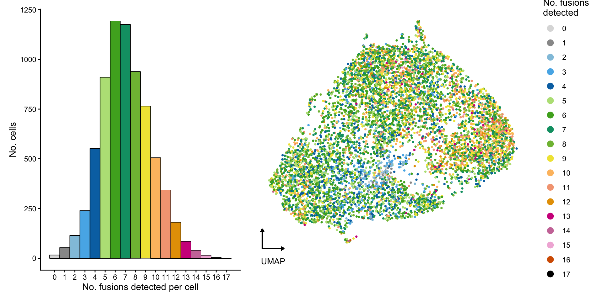
| Version | Author | Date |
|---|---|---|
| 1b5bb97 | Jovana Maksimovic | 2026-05-11 |
Fusion transcript expression (Figure 2A)
Violin plot showing normalised expression of all detected fusion transcripts, ordered by mean expression across cells. Each fusion is shown for all MCF7 cells, including zero-expression cells.
fusion_names <- rownames(seu)[str_detect(rownames(seu), "fusion") &
                                !(rownames(seu) %in% str_replace_all(unique(sce$patient_fusion), "_", "-"))]

fusion_data <- GetAssayData(seu, layer = "data")[fusion_names, ]

# Tidy to long format
fusion_long <- as.data.frame(t(as.matrix(fusion_data))) %>%
  rownames_to_column("cell") %>%
  pivot_longer(-cell, names_to = "fusion", values_to = "norm_expr")

# Order fusions by mean normalised expression (highest on top)
fusion_order <- fusion_long %>%
  group_by(fusion) %>%
  summarise(mean_expr = mean(norm_expr), .groups = "drop") %>%
  arrange(desc(mean_expr)) %>%
  pull(fusion)

fusion_long$fusion <- factor(fusion_long$fusion, levels = rev(fusion_order))

# Clean fusion labels: "GENE1-GENE2-fusion" → "GENE1::GENE2"
clean_label <- function(x) {
  x     <- str_remove(x, "-fusion$")
  parts <- str_split(x, "-")[[1]]
  paste0(parts[1], "::", parts[2])
}
label_map <- setNames(sapply(fusion_order, clean_label), fusion_order)

# Only colour the 3 fusions highlighted in Panel F (matched to that panel's
# own fusion colour), so A and F read as directly linked. Every other fusion
# gets a neutral grey fill instead of the previous full-gradient palette.
f_panel_colours <- c(
  "BCAS4-BCAS3-fusion"   = "#1A7A8A",
  "ARFGEF2-SULF2-fusion" = "#C0392B",
  "ZNF217-SULF2-fusion"  = "#7B3FA0"
)
fill_values_a <- setNames(rep("white", length(fusion_order)), fusion_order)
fill_values_a[names(f_panel_colours)] <- f_panel_colours

p_A <- ggplot(fusion_long, aes(x = fusion, y = norm_expr, fill = fusion)) +
  geom_jitter(data = fusion_long %>% filter(norm_expr > 0),
              aes(x = fusion, y = norm_expr),
              width = 0.25, size = 0.2, alpha = 0.1,
              color = "grey40", inherit.aes = FALSE) +
  geom_violin(scale = "width", trim = TRUE, linewidth = 0.3, color = "black", alpha = 0.5) +
  scale_fill_manual(values = fill_values_a, guide = "none") +
  scale_x_discrete(labels = label_map) +
  scale_y_continuous(expand = expansion(mult = c(0, 0.05))) +
  coord_flip() +
  labs(x = NULL, y = "Normalised expression",
       title = "MCF7 fusion expression") +
  theme_classic(base_size = 10) +
  theme(
    axis.text.y        = element_text(size = 8),
    axis.text.x        = element_text(size = 8),
    plot.title         = element_text(size = 11, face = "bold", color = "grey15", hjust = 0),
    panel.grid.major.x = element_line(color = "grey92", linewidth = 0.4)
  )

p_A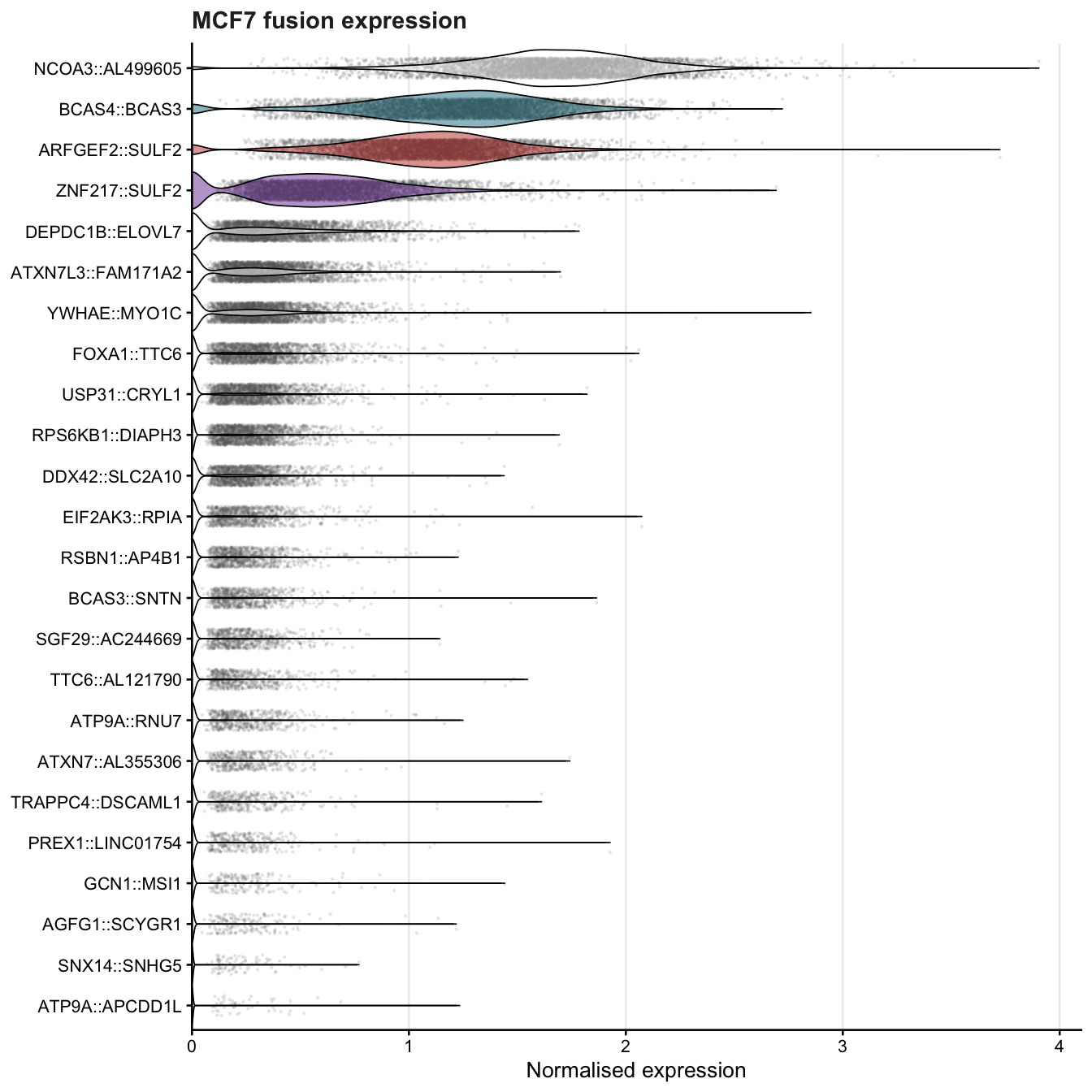
Key fusion expression vs. partner genes (Figure 2F)
Violin plots for three well-established MCF7 fusions — BCAS4::BCAS3, ARFGEF2::SULF2, and ZNF217::SULF2 — showing normalised expression of the fusion transcript alongside each partner gene. This illustrates that fusion transcripts are expressed at lower levels than their wildtype counterparts.
# Define the three well-established fusions and their partner genes
fusion_partners <- list(
  list(fusion_name  = "BCAS4-BCAS3-fusion",
       fusion_label = "BCAS4::BCAS3",
       gene1        = "BCAS4",
       gene2        = "BCAS3"),
  list(fusion_name  = "ARFGEF2-SULF2-fusion",
       fusion_label = "ARFGEF2::SULF2",
       gene1        = "ARFGEF2",
       gene2        = "SULF2"),
  list(fusion_name  = "ZNF217-SULF2-fusion",
       fusion_label = "ZNF217::SULF2",
       gene1        = "ZNF217",
       gene2        = "SULF2")
)

# Colour families: dark = fusion, mid = gene1, light = gene2
palette_families <- list(
  BCAS4_BCAS3   = c(fusion = "#1A7A8A", gene1 = "#57C4AD", gene2 = "#B8E4DC"),
  ARFGEF2_SULF2 = c(fusion = "#C0392B", gene1 = "#E8836F", gene2 = "#F5C5BD"),
  ZNF217_SULF2  = c(fusion = "#7B3FA0", gene1 = "#B07CC6", gene2 = "#DEC5ED")
)

# Helper: extract normalised expression for one fusion and its partners into long format
get_long_df <- function(f) {
  norm_data <- GetAssayData(seu, layer = "data")
  features  <- c(f$fusion_name, f$gene1, f$gene2)
  missing   <- features[!features %in% rownames(norm_data)]
  if (length(missing) > 0) {
    warning("Missing features: ", paste(missing, collapse = ", "))
    features <- features[features %in% rownames(norm_data)]
  }
  df <- as.data.frame(t(as.matrix(norm_data[features, , drop = FALSE])))
  if (f$fusion_name %in% colnames(df)) {
    df <- df %>% dplyr::rename(!!f$fusion_label := !!f$fusion_name)
  }
  df %>%
    rownames_to_column("cell") %>%
    pivot_longer(-cell, names_to = "feature", values_to = "norm_expr") %>%
    mutate(
      fusion_label = f$fusion_label,
      feature_type = case_when(
        feature == f$fusion_label ~ "fusion",
        feature == f$gene1        ~ "gene1",
        feature == f$gene2        ~ "gene2",
        TRUE                      ~ "other"
      ),
      feature = factor(feature, levels = c(f$fusion_label, f$gene1, f$gene2))
    )
}

# Helper: violin panel for one fusion + partners.
# `ylim`, if supplied, fixes the y-axis to a shared range across panels
# (used to put both SULF2 fusions on the same scale, per paper notes).
make_panel <- function(f, pal, ylim = NULL) {
  df         <- get_long_df(f)
  df_nonzero <- df %>% filter(norm_expr > 0)
  fill_values <- setNames(
    c(pal["fusion"], pal["gene1"], pal["gene2"]),
    c(f$fusion_label, f$gene1, f$gene2)
  )
  p <- ggplot(df, aes(x = feature, y = norm_expr, fill = feature)) +
    geom_jitter(data = df_nonzero, aes(x = feature, y = norm_expr),
                width = 0.15, size = 0.15, alpha = 0.25,
                color = "grey30", inherit.aes = FALSE) +
    geom_violin(scale = "width", trim = TRUE, linewidth = 0.3,
                color = "grey30", alpha = 0.85) +
    scale_fill_manual(values = fill_values, guide = "none") +
    # No per-panel title — the bold, coloured fusion name already on the
    # x-axis (below) identifies each panel, so a repeated heading above is
    # redundant.
    labs(x = NULL, y = "Normalised expression") +
    theme_classic(base_size = 9) +
    theme(
      axis.text.x        = element_text(size = 8, face = c("bold", "plain", "plain"),
                                        color = c(pal["fusion"], "grey20", "grey20"),
                                        angle = 30, hjust = 1),
      axis.text.y        = element_text(size = 8),
      axis.title.y       = element_text(size = 8),
      panel.grid.major.y = element_line(color = "grey94", linewidth = 0.3)
    )

  if (!is.null(ylim)) {
    p <- p + scale_y_continuous(limits = ylim, expand = expansion(mult = c(0, 0.08)))
  } else {
    p <- p + scale_y_continuous(expand = expansion(mult = c(0, 0.08)))
  }
  p
}

# ARFGEF2::SULF2 and ZNF217::SULF2 share the SULF2 partner gene, so they are
# put on a common y-axis scale to make their expression directly comparable.
# BCAS4::BCAS3 is unrelated and keeps its own auto-scaled y-axis.
sulf2_max <- max(
  get_long_df(fusion_partners[[2]])$norm_expr,
  get_long_df(fusion_partners[[3]])$norm_expr,
  na.rm = TRUE
)
sulf2_ylim <- c(0, sulf2_max)

panels <- list(
  make_panel(fusion_partners[[1]], palette_families[[1]]),
  make_panel(fusion_partners[[2]], palette_families[[2]], ylim = sulf2_ylim),
  make_panel(fusion_partners[[3]], palette_families[[3]], ylim = sulf2_ylim)
)

p_F <- wrap_plots(panels[1], ncol = 3) +
  plot_annotation(
    title = "Fusion vs. partner gene expression",
    # Matches fig2_title_theme in the "Combined Figure 2" section below
    # (same size/colour/alignment, plus a left margin so the "F" tag doesn't
    # overlap the title text once this panel is wrapped for assembly).
    theme = theme(plot.title = element_text(size = 11, face = "bold", color = "grey15",
                                            hjust = 0, margin = margin(l = 18, b = 4)))
  )

p_F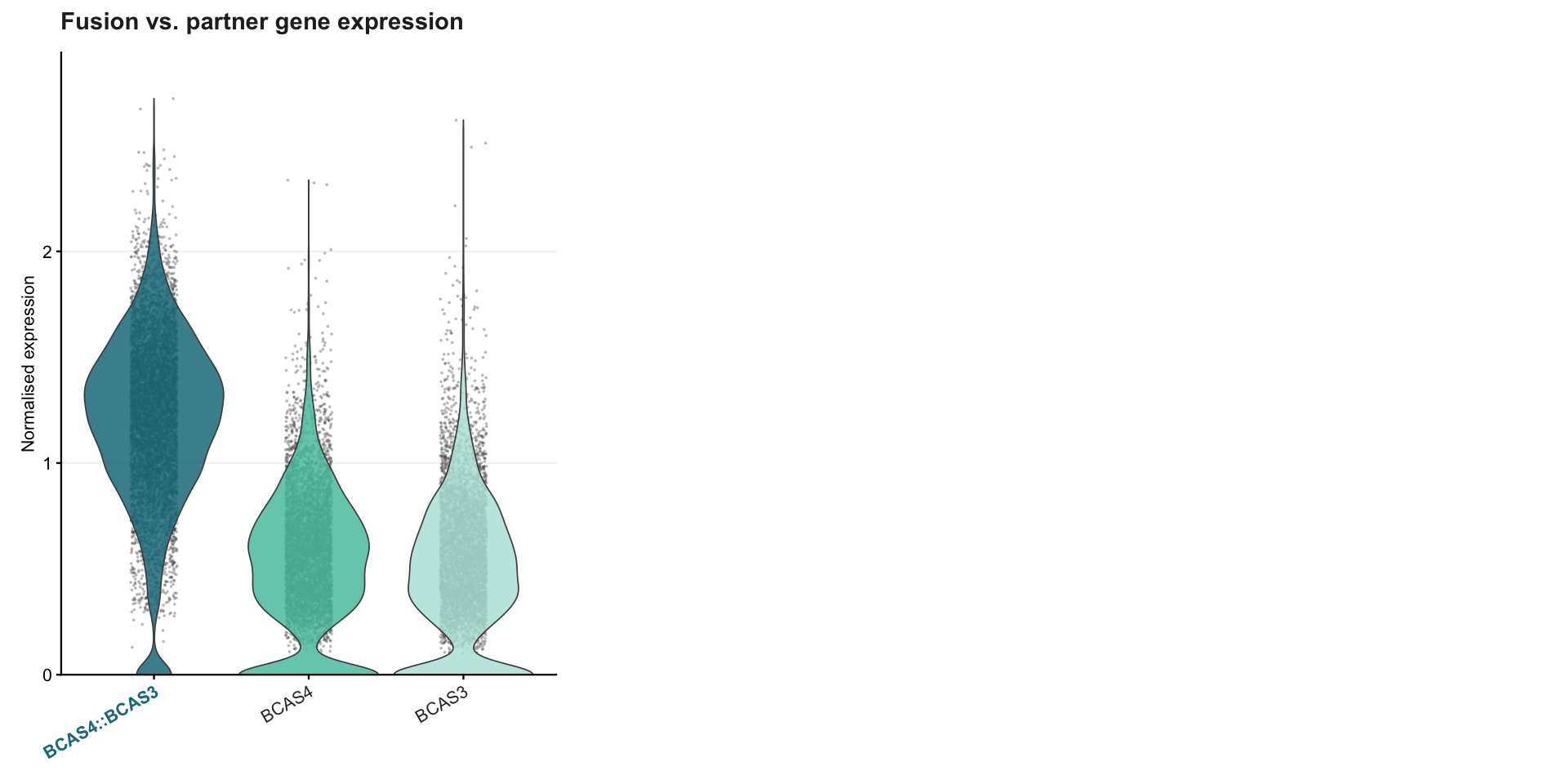
Cell cycle analysis (Supplementary Figure 1A–C)
MCF7 is a rapidly proliferating cell line. Here we assess whether cell cycle phase confounds fusion detection — for example, if S-phase cells happen to express more fusions due to higher overall transcriptional activity.
Cell cycle scoring
Score each cell for S-phase and G2M-phase gene expression using the Seurat built-in gene sets.
seu <- CellCycleScoring(seu,
                        s.features   = cc.genes$s.genes,
                        g2m.features = cc.genes$g2m.genes,
                        set.ident    = TRUE)
UMAP, fusion count, and library size by phase
phase_colours <- c("G2M" = "#4A6274", "S" = "#1A7A8A", "G1" = "#C0392B")

meta <- seu@meta.data %>%
  rownames_to_column("cell") %>%
  mutate(Phase = factor(Phase, levels = c("G1", "S", "G2M")))

# Ensure n_fusions_detected is present in metadata
if (!"n_fusions_detected" %in% colnames(meta)) {
  fusion_counts_cc <- GetAssayData(seu, layer = "counts")[
    rownames(seu)[str_detect(rownames(seu), "fusion")], ]
  meta <- meta %>%
    mutate(n_fusions_detected = colSums(fusion_counts_cc > 0)[cell])
}

# Kruskal-Wallis test: do phases differ in number of fusions detected?
kw <- kruskal.test(n_fusions_detected ~ Phase, data = meta)

format_pval_sci <- function(p, digits = 2) {
  sci   <- formatC(p, format = "e", digits = digits)
  parts <- strsplit(sci, "e")[[1]]
  sprintf("%s ~ '%s' ~ 10^%d", parts[1], "×", as.integer(parts[2]))
}

kw_label <- sprintf(
  "Kruskal-Wallis: italic(H) == %.2f ~ ',' ~ italic(p) == %s",
  kw$statistic,
  format_pval_sci(kw$p.value)
)

# UMAP axis coordinates
umap_coords  <- as.data.frame(seu@reductions$umap@cell.embeddings)
x_range_umap <- range(umap_coords[, 1])
y_range_umap <- range(umap_coords[, 2])
arrow_len_x  <- diff(x_range_umap) * 0.08
arrow_len_y  <- diff(y_range_umap) * 0.08

# Plot A: UMAP coloured by cell cycle phase
p_umap <- DimPlot(seu, group.by = "Phase", cols = phase_colours,
                  pt.size = 0.3, label = FALSE) +
  labs(title = "Cell cycle phase", colour = NULL) +
  theme_classic(base_size = 10) +
  theme(
    plot.title      = element_text(size = 10, face = "bold", color = "grey15"),
    legend.position = "bottom",
    legend.text     = element_text(size = 9),
    axis.title = element_blank(), axis.text  = element_blank(),
    axis.ticks = element_blank(), axis.line  = element_blank(),
    panel.grid = element_blank(), panel.border = element_blank()
  ) +
  geom_segment(aes(x = x_range_umap[1], xend = x_range_umap[1] + arrow_len_x,
                   y = y_range_umap[1], yend = y_range_umap[1]),
               arrow = arrow(length = unit(0.15, "cm"), type = "closed"),
               linewidth = 0.5, color = "black", inherit.aes = FALSE) +
  geom_segment(aes(x = x_range_umap[1], xend = x_range_umap[1],
                   y = y_range_umap[1], yend = y_range_umap[1] + arrow_len_y),
               arrow = arrow(length = unit(0.15, "cm"), type = "closed"),
               linewidth = 0.5, color = "black", inherit.aes = FALSE) +
  annotate("text", x = x_range_umap[1] + arrow_len_x / 2,
           y = y_range_umap[1] - diff(y_range_umap) * 0.04,
           label = "UMAP", size = 3, fontface = "italic", color = "grey30", hjust = 0.5)

# Plot B: fusions detected per cell by phase
p_fusions <- ggplot(meta, aes(x = Phase, y = n_fusions_detected, fill = Phase)) +
  geom_violin(scale = "width", trim = TRUE, linewidth = 0.3, color = "grey30", alpha = 0.85) +
  geom_boxplot(width = 0.12, fill = "white", color = "grey30",
               linewidth = 0.4, outlier.shape = NA) +
  annotate("text", x = 0.55, y = max(meta$n_fusions_detected) + 1,
           label = kw_label, parse = TRUE,
           hjust = 0, vjust = 1, size = 2.8, color = "grey30") +
  scale_fill_manual(values = phase_colours, guide = "none") +
  scale_y_continuous(expand = expansion(mult = c(0.02, 0.12))) +
  labs(x = "Cell cycle phase", y = "No. fusions detected per cell",
       title = "Fusions detected by phase") +
  theme_classic(base_size = 10) +
  theme(
    plot.title         = element_text(size = 10, face = "bold", color = "grey15", margin = margin(b = 8)),
    axis.title         = element_text(size = 9, color = "grey20"),
    axis.text          = element_text(size = 8, color = "grey30"),
    axis.line          = element_line(color = "grey60", linewidth = 0.4),
    axis.ticks         = element_line(color = "grey60", linewidth = 0.3),
    panel.grid.major.y = element_line(color = "grey95", linewidth = 0.4)
  )

# Plot C: library size by phase
p_library <- ggplot(meta, aes(x = Phase, y = nCount_RNA, fill = Phase)) +
  geom_violin(scale = "width", trim = TRUE, linewidth = 0.3, color = "grey30", alpha = 0.85) +
  geom_boxplot(width = 0.12, fill = "white", color = "grey30",
               linewidth = 0.4, outlier.shape = NA) +
  scale_fill_manual(values = phase_colours, guide = "none") +
  scale_y_continuous(labels = comma, expand = expansion(mult = c(0.02, 0.08))) +
  labs(x = "Cell cycle phase", y = "Total UMI count", title = "Library size by phase") +
  theme_classic(base_size = 10) +
  theme(
    plot.title         = element_text(size = 10, face = "bold", color = "grey15", margin = margin(b = 8)),
    axis.title         = element_text(size = 9, color = "grey20"),
    axis.text          = element_text(size = 8, color = "grey30"),
    axis.line          = element_line(color = "grey60", linewidth = 0.4),
    axis.ticks         = element_line(color = "grey60", linewidth = 0.3),
    panel.grid.major.y = element_line(color = "grey95", linewidth = 0.4)
  )

(p_umap | p_fusions | p_library) +
  plot_annotation(
    title = "Cell cycle phase and fusion detection in MCF7",
    theme = theme(plot.title = element_text(size = 11, face = "bold", color = "grey15", hjust = 0.5))
  ) +
  plot_layout(widths = c(1.4, 1, 1))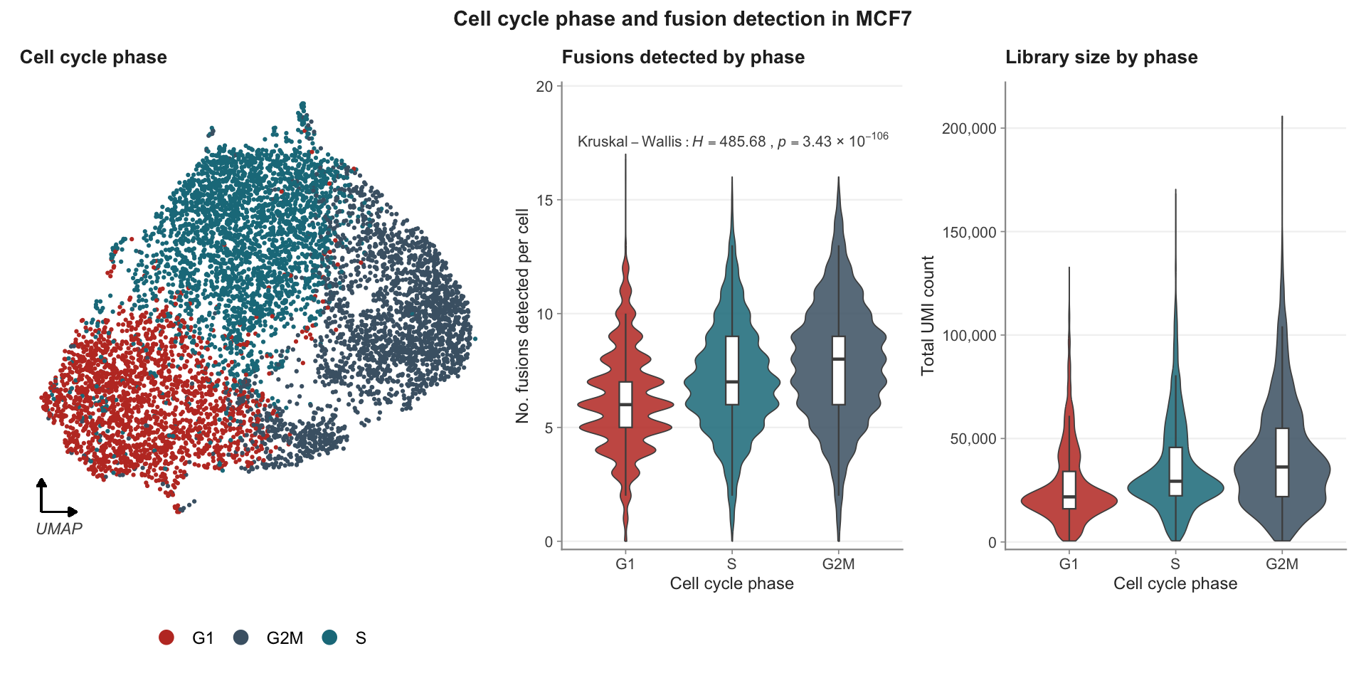
| Version | Author | Date |
|---|---|---|
| 1b5bb97 | Jovana Maksimovic | 2026-05-11 |
Fusion vs. partner gene expression (Supplementary Figure 1D)
For each detected fusion, compare the mean UMI per expressing cell between the fusion transcript and its two partner genes (5’ and 3’). This Cleveland dot plot shows that fusion transcripts are generally expressed at lower levels than their wildtype counterparts, consistent with fusions being detected by specific custom probes while partner gene expression is supported by the full endogenous probe set.
Identify wildtype partner genes
Extract the gene symbols of the 5’ and 3’ partner for each fusion from the fusion name string.
file  <- here("data", "RDS", "mcf7_fusion_stats.rds")
stats <- readRDS(file)

# Parse partner gene symbols from each fusion name
sapply(stats$fusion_list, function(f) {
  tmp <- strsplit(f, "-")[[1]]
  tmp <- tmp[tmp != "fusion"]
  tmp <- tmp[!grepl("^\\d+$", tmp)]
  tmp
}) -> fusion_partners_wt
Match each partner gene symbol to a feature in the Seurat object (some symbols may be absent if a partner gene is not covered by the probe set).
unlist(lapply(seq_along(fusion_partners_wt), function(i) {
  features <- c(names(fusion_partners_wt[i]), fusion_partners_wt[[i]])
  features <- rownames(seu)[rownames(seu) %in% features]
  features
})) -> all_features
Align wildtypes with fusions
Each fusion should have exactly two partner gene entries. When a partner gene is absent from the Seurat object, pad with NA so that the matrix has three columns (wildtype1, wildtype2, fusion).
list_of_fusion_pos <- which(grepl("fusion", all_features))

# Starting from index 2 (the first fusion is known to have 2 partners)
for (i in 2:length(list_of_fusion_pos)) {
  if ((list_of_fusion_pos[i] - list_of_fusion_pos[i - 1]) < 3) {
    all_features       <- append(all_features, NA, after = list_of_fusion_pos[i] - 1)
    list_of_fusion_pos <- which(grepl("fusion", all_features))
  }
}

wild_type_df <- as.data.frame(matrix(all_features, ncol = 3, byrow = TRUE))
colnames(wild_type_df) <- c("wild_type1", "wild_type2", "fusion")
Compute expression for each wildtype gene
# Mean UMI per expressing cell for a given gene (returns NA if gene absent)
identify_expression <- function(gene, seu) {
  if (is.na(gene)) return(c(NA, NA, NA))
  sum_reads          <- sum(seu[["RNA"]]$counts[gene, ])
  num_cells          <- sum(seu[["RNA"]]$counts[gene, ] > 0)
  expression_per_cell <- sum_reads / num_cells
  c(sum_reads, num_cells, expression_per_cell)
}

# Build a data frame of expression statistics for a list of genes
wildtype_expression_df <- function(wildtype_list, col_name, seu) {
  wildtype <- sapply(wildtype_list, identify_expression, seu)
  wildtype <- as.data.frame(t(wildtype))
  colnames(wildtype) <- c(
    glue("Sum_reads{col_name}"),
    glue("Num_cells{col_name}"),
    glue("Expression_per_cell{col_name}")
  )
  wildtype
}
wild_type_df <- wild_type_df %>%
cbind(wildtype_expression_df(wild_type_df$wild_type1, "_wild_type1", seu)) %>%
cbind(wildtype_expression_df(wild_type_df$wild_type2, "_wild_type2", seu)) %>%
cbind("Sum_reads_fusion" = stats$fusion_reads_mcf7) %>%
cbind("Num_cells_fusion" = stats$fusions_cell_nums) %>%
cbind("Expression_per_cell_fusion"= stats$average_reads_per_expressed_cell)
# Reorder columns: fusion first, then wildtype partners
ordering_colnames <- c(
which(grepl("fusion", colnames(wild_type_df))),
which(grepl("wild_type1", colnames(wild_type_df))),
which(grepl("wild_type2", colnames(wild_type_df)))
)
wild_type_df <- wild_type_df[ordering_colnames]Cleveland dot plot (Supplementary Figure 1D)
Each row is one fusion. The x-axis shows log₂ mean UMI per expressing cell; coloured dots indicate the fusion transcript (orange), 5’ partner (blue), and 3’ partner (sky blue). Fusions are ordered by fusion transcript expression.
wild_type_df_clean <- wild_type_df %>%
  mutate(
    clean_label = str_extract(fusion, "^[^-]+-[^-]+") %>%
      str_replace("-", "::"),
    clean_label = fct_reorder(clean_label, log2(Expression_per_cell_fusion))
  ) %>%
  rowwise() %>%
  mutate(
    x_min = min(log2(Expression_per_cell_fusion),
                log2(Expression_per_cell_wild_type1),
                log2(Expression_per_cell_wild_type2),
                na.rm = TRUE),
    x_max = max(log2(Expression_per_cell_fusion),
                log2(Expression_per_cell_wild_type1),
                log2(Expression_per_cell_wild_type2),
                na.rm = TRUE)
  ) %>%
  ungroup()

dot_colours <- c(
  "Fusion transcript" = "#D55E00",
  "5' partner"        = "#0072B2",
  "3' partner"        = "#56B4E9"
)

p_supp2 <- ggplot(wild_type_df_clean) +
  geom_linerange(aes(y = clean_label, xmin = x_min, xmax = x_max),
                 color = "grey80", linewidth = 0.4) +
  geom_point(aes(x = log2(Expression_per_cell_wild_type1), y = clean_label, color = "5' partner"),
             size = 2.5, alpha = 0.9) +
  geom_point(aes(x = log2(Expression_per_cell_wild_type2), y = clean_label, color = "3' partner"),
             size = 2.5, alpha = 0.9) +
  geom_point(aes(x = log2(Expression_per_cell_fusion), y = clean_label, color = "Fusion transcript"),
             size = 2.5, alpha = 0.9) +
  scale_color_manual(values = dot_colours, name = NULL,
                     guide = guide_legend(override.aes = list(size = 3))) +
  scale_x_continuous(expand = expansion(mult = c(0.05, 0.1))) +
  labs(
    x     = expression(log[2] ~ "(Mean UMI per expressing cell)"),
    y     = NULL,
    title = "Fusion transcript expression relative to partner genes"
  ) +
  theme_classic(base_size = 10) +
  theme(
    plot.title         = element_text(size = 10, face = "bold", color = "grey15", margin = margin(b = 8)),
    plot.margin        = margin(8, 16, 8, 8),
    axis.title.x       = element_text(size = 9, color = "grey20", margin = margin(t = 6)),
    axis.text.y        = element_text(size = 8, color = "grey20"),
    axis.text.x        = element_text(size = 8, color = "grey30"),
    axis.line          = element_line(color = "grey60", linewidth = 0.4),
    axis.ticks         = element_line(color = "grey60", linewidth = 0.3),
    panel.grid.major.x = element_line(color = "grey95", linewidth = 0.4),
    panel.grid.major.y = element_line(color = "grey95", linewidth = 0.3),
    legend.position    = "bottom",
    legend.text        = element_text(size = 9),
    legend.key.size    = unit(0.5, "lines")
  )

p_supp2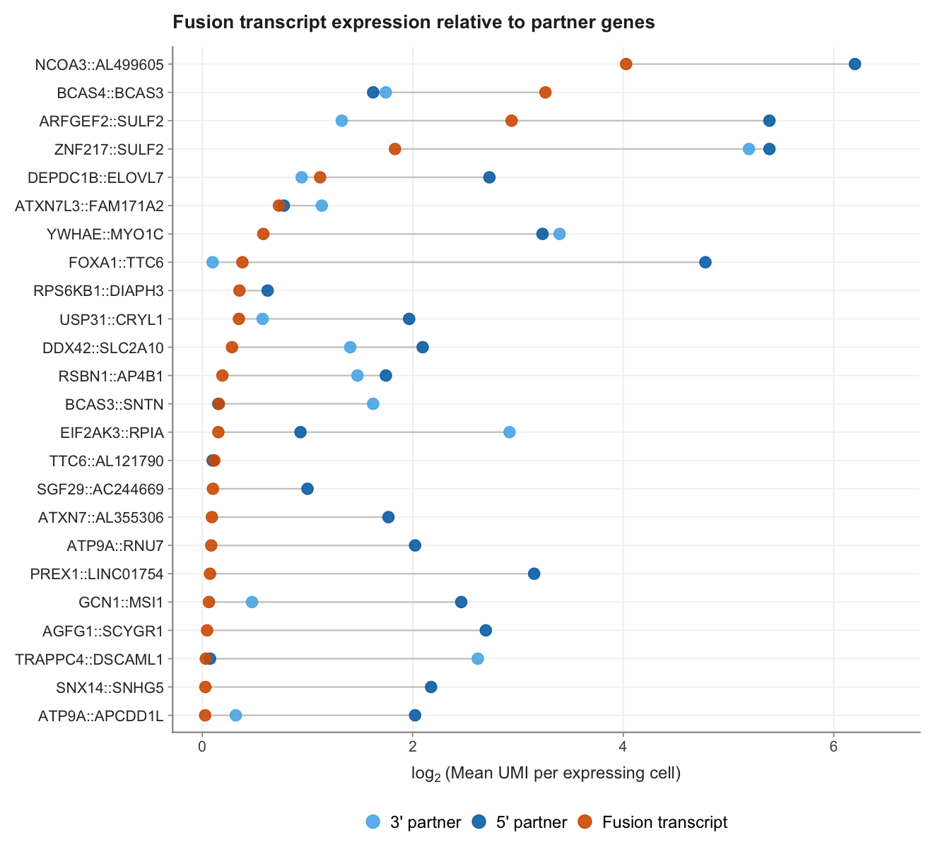
| Version | Author | Date |
|---|---|---|
| 1b5bb97 | Jovana Maksimovic | 2026-05-11 |
Save wildtype comparison table
out <- here("data", "RDS", "mcf7_wt_comparison.rds")
if (!file.exists(out)) saveRDS(wild_type_df, out)
Combined Figure 2
Panels D and E reuse the per-fusion statistics table from
MCF7_exp1_probe_quality.Rmd. They are rebuilt here as
standalone objects so all six panels (A–F) can be assembled into a
single patchwork figure. No files are exported at this
stage.
Load fusion statistics table
fig2_stats_file <- here("data", "RDS", "mcf7_fusion_stats.rds")
fig2_stats      <- readRDS(fig2_stats_file)
Panel D: single-cell UMI count vs. number of cells with fusion detected
# Label the top 10 fusions by mean MCF7 expression (same ordering as Panel
# A's `fusion_order`) — a single, objective rule shared with Panel E, rather
# than two different hand-picked lists (previously 4 fusions here, 6 in E,
# for no stated reason).
top10_fusions <- head(fusion_order, 10)

stats_clean_d <- fig2_stats %>%
  { if (!"fusion_id" %in% colnames(.)) rownames_to_column(., "fusion_id") else . } %>%
  mutate(
    clean_label = str_extract(fusion_id, "^[^-]+-[^-]+") %>%
      str_replace("-", "::"),
    established = fusion_id %in% top10_fusions
  )

m_d         <- lm(log2(fusion_reads_mcf7) ~ log2(fusions_cell_nums), stats_clean_d)
intercept_d <- coef(m_d)[1]
slope_d     <- coef(m_d)[2]
r_sq_d      <- summary(m_d)$r.squared
resid_sd_d  <- sd(residuals(m_d))

cor_d <- cor.test(
  stats_clean_d$fusions_cell_nums,
  stats_clean_d$fusion_reads_mcf7,
  method = "spearman",
  exact  = FALSE
)

x_range_d <- range(log2(stats_clean_d$fusions_cell_nums))
ribbon_d  <- data.frame(x = seq(x_range_d[1], x_range_d[2], length.out = 200)) %>%
  mutate(
    fitted = intercept_d + slope_d * x,
    sd1_hi = fitted + 1 * resid_sd_d,
    sd1_lo = fitted - 1 * resid_sd_d,
    sd2_hi = fitted + 2 * resid_sd_d,
    sd2_lo = fitted - 2 * resid_sd_d
  )

r_sq_label_d <- sprintf("italic(R)^2 == %.2f", r_sq_d)
# NB: a raw "%.2e" value (e.g. "1.23e-10") embedded in a parse()d plotmath
# string is displayed in full decimal form, not scientific notation, because
# this document sets options(scipen = 999) in the setup chunk — R's plotmath
# deparser respects that option when it renders the numeric literal, which is
# why this label previously showed a long run of zeros instead of "p = 1.2 ×
# 10^-10". format_pval_sci() (defined above, in the cell cycle section) sidesteps
# this by building the scientific notation as explicit text/exponent pieces
# rather than a numeric literal, exactly as already used for the
# Kruskal-Wallis p-value label.
rho_label_d  <- sprintf(
  "italic(ρ) == %.3f ~ ',' ~ italic(p) == %s",
  cor_d$estimate,
  format_pval_sci(cor_d$p.value)
)
x_annot_d <- x_range_d[1] + 0.1
y_annot_d <- max(log2(stats_clean_d$fusion_reads_mcf7))

p_D <- ggplot(stats_clean_d,
       aes(x = log2(fusions_cell_nums), y = log2(fusion_reads_mcf7))) +
  # SD bands: grey shades (was teal), mapped to `fill` so they get a proper
  # legend instead of in-plot "±1 SD"/"±2 SD" text — the old text sat right
  # on top of the data in the bottom-left corner.
  geom_ribbon(data = ribbon_d, aes(x = x, ymin = sd2_lo, ymax = sd2_hi, fill = "±2 SD"),
              alpha = 0.35, inherit.aes = FALSE) +
  geom_ribbon(data = ribbon_d, aes(x = x, ymin = sd1_lo, ymax = sd1_hi, fill = "±1 SD"),
              alpha = 0.45, inherit.aes = FALSE) +
  geom_line(data = ribbon_d, aes(x = x, y = fitted),
            color = "grey30", linetype = "dashed", linewidth = 0.6, inherit.aes = FALSE) +
  # Uniform point size — the y axis already shows UMI count (expression
  # level), so a separate size encoding for "established" fusions is
  # redundant here (unlike E, which keeps it).
  geom_point(size = 2.2, shape = 21, fill = "black", color = "white", stroke = 0.3, alpha = 0.85) +
  # geom_text_repel (not geom_text + fixed nudge) — the top-expressed points
  # cluster at the far right (highest UMI counts), so fixed nudges pushed
  # labels like "NCOA3::AL499605" past the plot's right edge and clipped
  # them. repel keeps every label within the panel (matches Panel E).
  geom_text_repel(data = stats_clean_d %>% filter(established), aes(label = clean_label),
                  size = 2.25, color = "black", seed = 1, min.segment.length = 0,
                  segment.size = 0.25, segment.color = "grey60",
                  box.padding = 0.35, max.overlaps = Inf,
                  xlim = c(NA, x_range_d[2])) +
  annotate("text", x = x_annot_d, y = y_annot_d - 0.3,
           label = r_sq_label_d, parse = TRUE, hjust = 0, vjust = 1, size = 3.2, color = "grey30") +
  annotate("text", x = x_annot_d, y = y_annot_d - 1.1,
           label = rho_label_d, parse = TRUE, hjust = 0, vjust = 1, size = 3.2, color = "grey30") +
  scale_fill_manual(
    name   = NULL,
    breaks = c("±1 SD", "±2 SD"),
    values = c("±1 SD" = "grey55", "±2 SD" = "grey82"),
    guide  = guide_legend(override.aes = list(alpha = 1))
  ) +
  coord_cartesian(clip = "off") +
  labs(
    x     = expression(log[2] ~ "(No. cells with fusion detected)"),
    y     = expression(log[2] ~ "(Single-cell fusion UMI count)"),
    title = "UMI count vs. cells with fusion detected"
  ) +
  theme_classic(base_size = 10) +
  theme(
    plot.title       = element_text(size = 11, face = "bold", color = "grey15", hjust = 0, margin = margin(b = 8)),
    plot.margin      = margin(12, 20, 8, 8),
    axis.title       = element_text(size = 9, color = "grey20"),
    axis.title.x     = element_text(margin = margin(t = 6)),
    axis.title.y     = element_text(margin = margin(r = 6)),
    axis.text        = element_text(size = 8, color = "grey30"),
    axis.line        = element_line(color = "grey60", linewidth = 0.4),
    axis.ticks       = element_line(color = "grey60", linewidth = 0.3),
    panel.grid.major = element_line(color = "grey95", linewidth = 0.4),
    panel.grid.minor = element_blank(),
    legend.position  = "bottom",
    legend.direction = "horizontal",
    legend.text      = element_text(size = 7.5),
    legend.key.size  = unit(0.6, "lines"),
    legend.margin    = margin(t = -6)
  )

p_D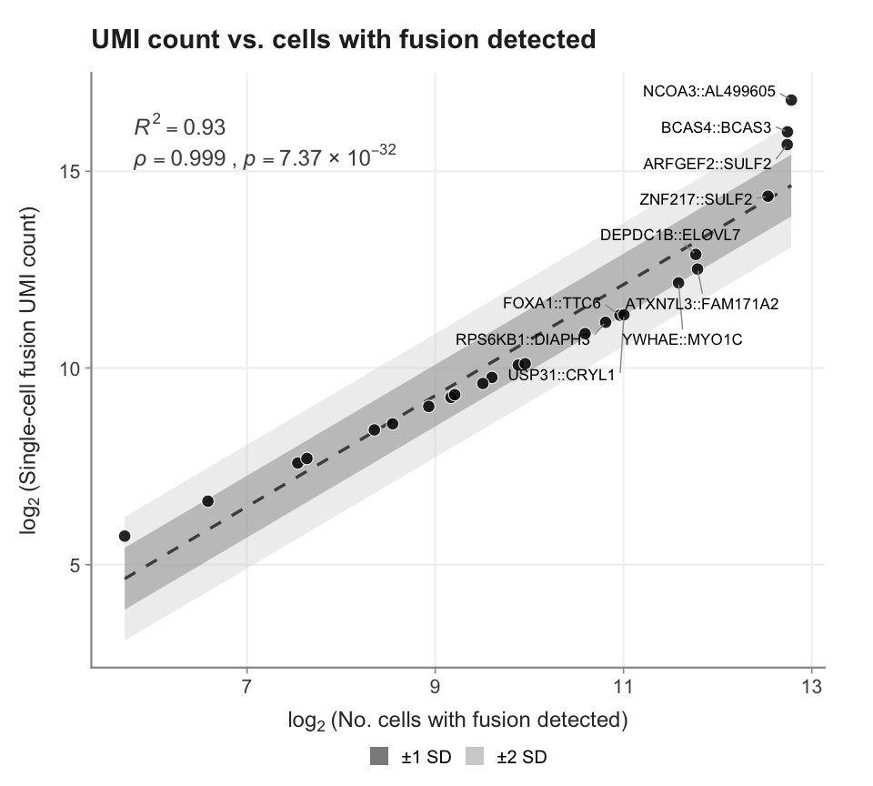
| Version | Author | Date |
|---|---|---|
| e69a9f3 | Jovana Maksimovic | 2026-07-15 |
Panel E: concordance between bulk (Arriba) and single-cell fusion detection
# Same top-10-by-expression rule as Panel D (see comment there) — keeps the
# labelled fusions consistent between the two correlation panels.
stats_clean_e <- fig2_stats %>%
  { if (!"fusion_id" %in% colnames(.)) rownames_to_column(., "fusion_id") else . } %>%
  mutate(
    clean_label = str_extract(fusion_id, "^[^-]+-[^-]+") %>%
      str_replace("-", "::"),
    established = fusion_id %in% top10_fusions
  )

m_e         <- lm(log2(fusion_reads_mcf7) ~ log2(average_sum_split_reads), stats_clean_e)
intercept_e <- coef(m_e)[1]
slope_e     <- coef(m_e)[2]
r_sq_e      <- summary(m_e)$r.squared
resid_sd_e  <- sd(residuals(m_e))

cor_e <- cor.test(
  stats_clean_e$average_sum_split_reads,
  stats_clean_e$fusion_reads_mcf7,
  method = "spearman",
  exact  = FALSE
)

x_range_e <- range(log2(stats_clean_e$average_sum_split_reads))
ribbon_e  <- data.frame(x = seq(x_range_e[1], x_range_e[2], length.out = 200)) %>%
  mutate(
    fitted = intercept_e + slope_e * x,
    sd1_hi = fitted + 1 * resid_sd_e,
    sd1_lo = fitted - 1 * resid_sd_e,
    sd2_hi = fitted + 2 * resid_sd_e,
    sd2_lo = fitted - 2 * resid_sd_e
  )

r_sq_label_e <- sprintf("italic(R)^2 == %.2f", r_sq_e)
rho_label_e  <- sprintf(
  "italic(ρ) == %.2f ~ ',' ~ p == %.3f",
  cor_e$estimate,
  cor_e$p.value
)
x_annot_e <- x_range_e[1] + 0.2
y_annot_e <- max(log2(stats_clean_e$fusion_reads_mcf7))

p_E <- ggplot(stats_clean_e,
       aes(x = log2(average_sum_split_reads), y = log2(fusion_reads_mcf7))) +
  # SD bands: grey shades (was teal), mapped to `fill` so they get a proper
  # legend instead of in-plot "±1 SD"/"±2 SD" text (matches Panel D).
  geom_ribbon(data = ribbon_e, aes(x = x, ymin = sd2_lo, ymax = sd2_hi, fill = "±2 SD"),
              alpha = 0.35, inherit.aes = FALSE) +
  geom_ribbon(data = ribbon_e, aes(x = x, ymin = sd1_lo, ymax = sd1_hi, fill = "±1 SD"),
              alpha = 0.45, inherit.aes = FALSE) +
  geom_line(data = ribbon_e, aes(x = x, y = fitted),
            color = "grey30", linetype = "dashed", linewidth = 0.6, inherit.aes = FALSE) +
  geom_point(aes(size = established),
             shape = 21, fill = "black", color = "white", stroke = 0.3, alpha = 0.85) +
  scale_size_manual(values = c("TRUE" = 3, "FALSE" = 2), guide = "none") +
  # geom_text_repel (not geom_text + manual nudge) — with 10 labelled points,
  # fixed nudges caused overlaps (e.g. BCAS4::BCAS3/ARFGEF2::SULF2); repel
  # resolves that automatically. xlim keeps labels from being pushed past
  # the plot's right edge and clipped (matches Panel D).
  geom_text_repel(data = stats_clean_e %>% filter(established), aes(label = clean_label),
                  size = 2.25, color = "black", seed = 1, min.segment.length = 0,
                  segment.size = 0.25, segment.color = "grey60",
                  box.padding = 0.35, max.overlaps = Inf,
                  xlim = c(NA, x_range_e[2])) +
  annotate("text", x = x_annot_e, y = y_annot_e - 0.3,
           label = r_sq_label_e, parse = TRUE, hjust = 0, vjust = 1, size = 3.2, color = "grey30") +
  annotate("text", x = x_annot_e, y = y_annot_e - 1.1,
           label = rho_label_e, parse = TRUE, hjust = 0, vjust = 1, size = 3.2, color = "grey30") +
  scale_fill_manual(
    name   = NULL,
    breaks = c("±1 SD", "±2 SD"),
    values = c("±1 SD" = "grey55", "±2 SD" = "grey82"),
    guide  = guide_legend(override.aes = list(alpha = 1))
  ) +
  labs(
    x     = expression(log[2] ~ "(Arriba split read count)"),
    y     = expression(log[2] ~ "(Single-cell fusion UMI count)"),
    title = "Bulk vs. single-cell concordance"
  ) +
  theme_classic(base_size = 10) +
  coord_cartesian(clip = "off") +
  theme(
    plot.title       = element_text(size = 11, face = "bold", color = "grey15", hjust = 0, margin = margin(b = 8)),
    plot.margin      = margin(12, 20, 8, 8),
    axis.title       = element_text(size = 9, color = "grey20"),
    axis.title.x     = element_text(margin = margin(t = 6)),
    axis.title.y     = element_text(margin = margin(r = 6)),
    axis.text        = element_text(size = 8, color = "grey30"),
    axis.line        = element_line(color = "grey60", linewidth = 0.4),
    axis.ticks       = element_line(color = "grey60", linewidth = 0.3),
    panel.grid.major = element_line(color = "grey95", linewidth = 0.4),
    panel.grid.minor = element_blank(),
    legend.position  = "bottom",
    legend.direction = "horizontal",
    legend.text      = element_text(size = 7.5),
    legend.key.size  = unit(0.6, "lines"),
    legend.margin    = margin(t = -6)
  )

p_E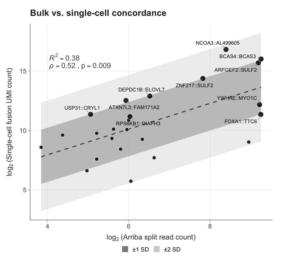
| Version | Author | Date |
|---|---|---|
| e69a9f3 | Jovana Maksimovic | 2026-07-15 |
Assemble all six panels
Three independently-sized rows, stacked: A/B/C, then D/E (each 50%
width), then F alone across the full width. This differs from the
current manual arrangement in
output/flex_fusion_figures.pptx (slide 2), which packs
D/E/F into a single row — that layout left F too wide and D/E uneven, so
panel F now gets its own row.
# Shared heading style: same size, bold, left-aligned for every panel title
# (previously inconsistent — A/D/E were ~10-11pt, F was 12pt and centred;
# B/C had no title at all). A left margin is added so the tag (drawn at the
# panel's top-left corner) never overlaps the title text — this was most
# visible on C, where "C" + "Fusion..." rendered as "Cusion...".
fig2_title_theme <- theme(
  plot.title = element_text(size = 11, face = "bold", color = "grey15",
                            hjust = 0, margin = margin(l = 18, b = 4))
)

# B and C had no panel titles before — add them so every panel is labelled.
p_B <- p_B + labs(title = "Fusions detected per cell")     + fig2_title_theme
p_C <- p_C + labs(title = "Fusion count per cell (UMAP)")  + fig2_title_theme
p_A <- p_A + fig2_title_theme
p_D <- p_D + fig2_title_theme
p_E <- p_E + fig2_title_theme
# p_F's title is set inside its own plot_annotation() (it's a nested
# patchwork of 3 sub-panels, not a single ggplot) — already matched to
# fig2_title_theme's size/colour/alignment where p_F is built above.

# As in `B-ALL_exp1_clustering.Rmd`, the tag (A/B/C/D/E/F) theme is applied
# to each panel individually rather than via `& theme(...)` on the combined
# patchwork — patchwork reads `plot.tag` from each panel's own theme, and
# relying on `&` for this is unreliable across patchwork versions (it also
# collides with the Matrix package's S4 Ops methods loaded by Seurat).
# This also makes the tag size trivial to resize later: change tag_theme
# once here rather than hunting through plot_annotation() calls.
tag_theme <- theme(plot.tag = element_text(size = 18, face = "bold"))

# A, C, D, E, and F are each wrapped with wrap_elements(full = ...) before
# being tagged/added to the patchwork, for three reasons:
#  1. p_F is itself a nested patchwork (3 sub-panels). Without wrapping,
#     tag_levels = "A" recurses into it and tags the sub-panels individually
#     (giving F/G/H instead of a single F) — wrap_elements() treats it as one
#     opaque patch so it gets exactly one tag.
#  2. C (custom arrow-based UMAP axes) and D/E (annotation text near the
#     plot edges) were being stretched/padded when patchwork tried to align
#     their axes with neighbouring panels, producing large gaps between axis
#     titles and axes, and titles bleeding into adjacent panels.
#     wrap_elements() freezes each as a fixed-size image so it is placed in
#     its grid cell without that cross-panel alignment.
#  3. A's title text is long enough to overflow past its (narrow) column
#     into B's column, since ggplot doesn't clip title text to the panel
#     width by default. Wrapping clips it to A's own grid cell.
# B is left unwrapped — it's a plain bar chart with no axis/legend quirks
# and no observed overflow, so wrapping isn't needed.
p_A_tag <- wrap_elements(full = p_A) + tag_theme
p_B_tag <- p_B + tag_theme
p_C_tag <- wrap_elements(full = p_C) + tag_theme
p_D_tag <- wrap_elements(full = p_D) + tag_theme
p_E_tag <- wrap_elements(full = p_E) + tag_theme
p_F_tag <- wrap_elements(full = p_F) + tag_theme

# Rows are assembled as THREE separate patchwork objects, each with its own
# `widths` vector, then stacked with `/`. A single shared-column design (as
# used previously) forces every row to use the same column widths — that's
# why A/F couldn't be resized independently of D/E and B/C. Building each
# row on its own decouples them completely:
#  - Row 1: A narrower; B and C wider (B's axis labels and C's legend need
#    the room).
#  - Row 2: D and E only, each exactly 50% of the row.
#  - Row 3: F alone, full width (previously squeezed next to D/E).
row1 <- p_A_tag + p_B_tag + p_C_tag +
  plot_layout(widths = c(0.8, 1, 1))

row2 <- p_D_tag + p_E_tag +
  plot_layout(widths = c(1, 1))

row3 <- p_F_tag

figure2 <- (row1 / row2 / row3) +
  plot_layout(heights = c(1.3, 1, 1)) +
  plot_annotation(tag_levels = "A")

figure2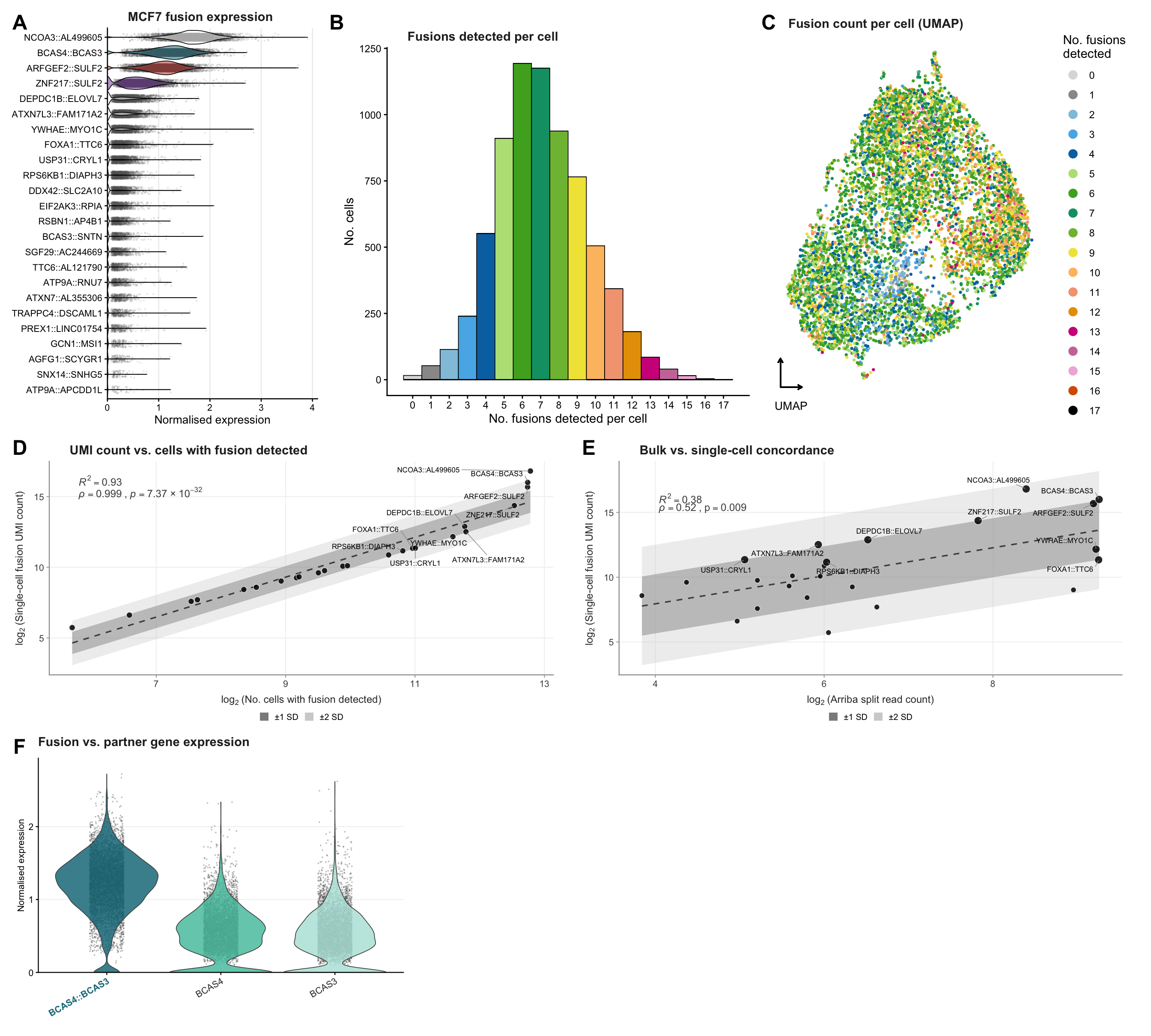
| Version | Author | Date |
|---|---|---|
| e69a9f3 | Jovana Maksimovic | 2026-07-15 |
Combined Supplementary Figure 1
Assembles all four panels of Supplementary Figure 1: panels A–C are
the cell cycle plots (UMAP, fusions detected by phase, library size by
phase) built in the section above; panel D is the Cleveland dot plot of
fusion vs. partner gene expression. Follows the same conventions as
Figure 2: tags applied per-panel via tag_theme, not via
&, and a left margin on each title to prevent the tag
overlapping the text.
Unlike Figure 2’s panel F, none of these four panels are themselves a
nested patchwork, so no wrap_elements() is needed —
tag_levels tags all four leaves (A–D) directly.
# p_umap / p_fusions / p_library here are the CELL CYCLE versions built in
# the "plot-cell-cycle" chunk above — that chunk is the last thing in the
# document to assign these (deliberately generic, reused) names before this
# point, so it's safe to pick them up directly. Renamed here for clarity now
# that they're becoming panels of a combined supplementary figure.
p_supp1a <- p_umap
p_supp1b <- p_fusions
p_supp1c <- p_library
# p_supp2 (the Cleveland dot plot) was captured directly in the
# "plot-wildtype-cleveland" chunk above.

title_margin_fix <- theme(plot.title = element_text(margin = margin(l = 18)))
# `tag_theme` (size = 18, bold) was already defined in the fig2-assemble
# chunk above and is reused here as-is, for the same tag size/style
# throughout the whole notebook.
p_supp1a <- p_supp1a + title_margin_fix + tag_theme
p_supp1b <- p_supp1b + title_margin_fix + tag_theme
p_supp1c <- p_supp1c + title_margin_fix + tag_theme
p_supp2  <- p_supp2  + title_margin_fix + tag_theme

suppfig_row1 <- p_supp1a + p_supp1b + p_supp1c +
  plot_layout(widths = c(1.4, 1, 1))

# supp_figure <- (suppfig_row1 / p_supp2) +
#   plot_layout(heights = c(1, 1.3)) +
#   plot_annotation(tag_levels = "A")

supp_figure <- (suppfig_row1) +
  plot_layout(heights = c(1)) +
  plot_annotation(tag_levels = "A")

supp_figure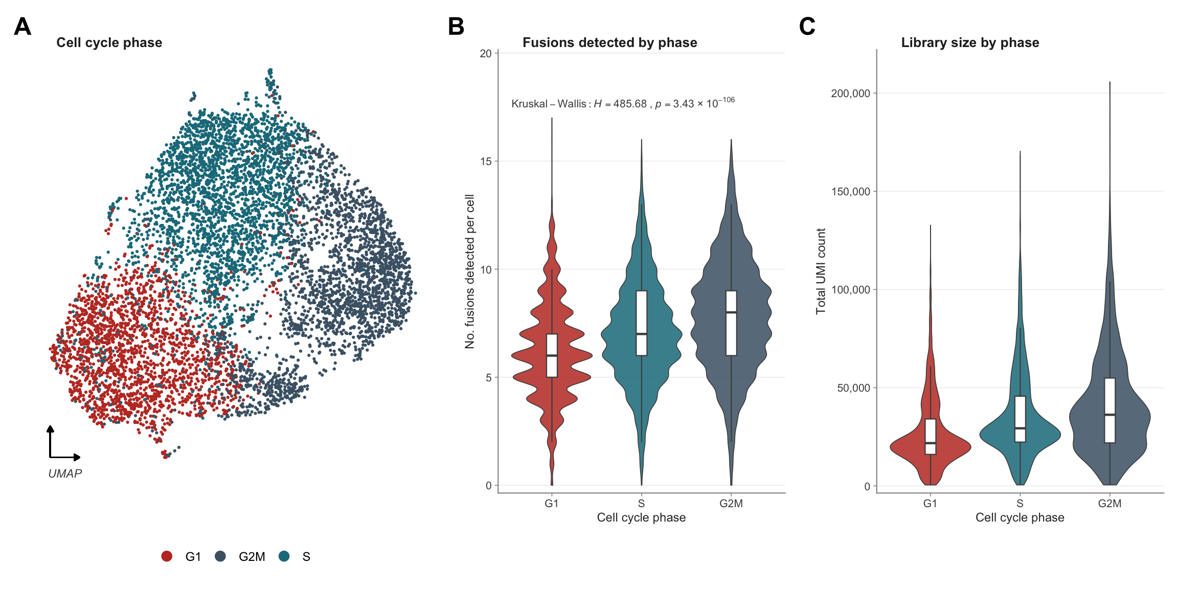
| Version | Author | Date |
|---|---|---|
| e69a9f3 | Jovana Maksimovic | 2026-07-15 |
Session info
sessioninfo::session_info()─ Session info ───────────────────────────────────────────────────────────────
setting value
version R version 4.4.1 (2024-06-14)
os macOS 15.7.9
system aarch64, darwin20
ui X11
language (EN)
collate en_US.UTF-8
ctype en_US.UTF-8
tz Australia/Melbourne
date 2026-08-25
pandoc 3.8.3 @ /Applications/RStudio.app/Contents/Resources/app/quarto/bin/tools/aarch64/ (via rmarkdown)
quarto 1.9.38 @ /Applications/RStudio.app/Contents/Resources/app/quarto/bin/quarto
─ Packages ───────────────────────────────────────────────────────────────────
! package * version date (UTC) lib source
P abind 1.4-8 2024-09-12 [?] CRAN (R 4.4.1)
P Biobase * 2.66.0 2024-11-08 [?] Bioconduc~
P BiocGenerics * 0.52.0 2024-11-08 [?] Bioconduc~
P BiocManager 1.30.27 2025-11-14 [?] CRAN (R 4.4.3)
P bslib 0.9.0 2025-01-30 [?] CRAN (R 4.4.1)
P cachem 1.1.0 2024-05-16 [?] CRAN (R 4.4.1)
P callr 3.7.6 2024-03-25 [?] CRAN (R 4.4.0)
P cli 3.6.5 2025-04-23 [?] CRAN (R 4.4.1)
P cluster 2.1.6 2023-12-01 [?] CRAN (R 4.4.1)
P codetools 0.2-20 2024-03-31 [?] CRAN (R 4.4.1)
P colorspace 2.1-1 2024-07-26 [?] CRAN (R 4.4.1)
P cowplot 1.1.3 2024-01-22 [?] CRAN (R 4.4.0)
P crayon 1.5.3 2024-06-20 [?] CRAN (R 4.4.1)
P data.table 1.18.2.1 2026-01-27 [?] CRAN (R 4.4.3)
P DelayedArray 0.32.0 2024-11-08 [?] Bioconduc~
P deldir 2.0-4 2024-02-28 [?] CRAN (R 4.4.1)
P digest 0.6.37 2024-08-19 [?] CRAN (R 4.4.1)
P dotCall64 1.2 2024-10-04 [?] CRAN (R 4.4.1)
P dplyr * 1.1.4 2023-11-17 [?] CRAN (R 4.4.0)
P evaluate 1.0.3 2025-01-10 [?] CRAN (R 4.4.1)
P farver 2.1.2 2024-05-13 [?] CRAN (R 4.4.1)
P fastDummies 1.7.5 2025-01-20 [?] CRAN (R 4.4.1)
P fastmap 1.2.0 2024-05-15 [?] CRAN (R 4.4.1)
P fitdistrplus 1.2-2 2025-01-07 [?] CRAN (R 4.4.1)
P forcats * 1.0.0 2023-01-29 [?] CRAN (R 4.4.0)
P fs 1.6.6 2025-04-12 [?] CRAN (R 4.4.1)
P future 1.49.0 2025-05-09 [?] CRAN (R 4.4.1)
P future.apply 1.11.3 2024-10-27 [?] CRAN (R 4.4.1)
P generics 0.1.4 2025-05-09 [?] CRAN (R 4.4.1)
P GenomeInfoDb * 1.42.3 2025-01-27 [?] Bioconduc~
P GenomeInfoDbData 1.2.13 2025-05-28 [?] Bioconductor
P GenomicRanges * 1.58.0 2024-11-08 [?] Bioconduc~
P getPass 0.2-4 2023-12-10 [?] CRAN (R 4.4.1)
P ggplot2 * 4.0.2 2026-02-03 [?] CRAN (R 4.4.3)
P ggrepel * 0.9.6 2024-09-07 [?] CRAN (R 4.4.1)
P ggridges 0.5.6 2024-01-23 [?] CRAN (R 4.4.0)
P git2r 0.36.2 2025-03-29 [?] CRAN (R 4.4.1)
P globals 0.18.0 2025-05-08 [?] CRAN (R 4.4.1)
P glue * 1.8.0 2024-09-30 [?] CRAN (R 4.4.1)
P goftest 1.2-3 2021-10-07 [?] CRAN (R 4.4.1)
P gridExtra 2.3 2017-09-09 [?] CRAN (R 4.4.1)
P gtable 0.3.6 2024-10-25 [?] CRAN (R 4.4.1)
P here * 1.0.1 2020-12-13 [?] CRAN (R 4.4.1)
P hms 1.1.3 2023-03-21 [?] CRAN (R 4.4.0)
P htmltools 0.5.8.1 2024-04-04 [?] CRAN (R 4.4.1)
P htmlwidgets 1.6.4 2023-12-06 [?] CRAN (R 4.4.0)
P httpuv 1.6.16 2025-04-16 [?] CRAN (R 4.4.1)
P httr 1.4.7 2023-08-15 [?] CRAN (R 4.4.0)
P ica 1.0-3 2022-07-08 [?] CRAN (R 4.4.1)
P igraph 2.1.4 2025-01-23 [?] CRAN (R 4.4.1)
P IRanges * 2.40.1 2024-12-05 [?] Bioconduc~
P irlba 2.3.5.1 2022-10-03 [?] CRAN (R 4.4.0)
P jquerylib 0.1.4 2021-04-26 [?] CRAN (R 4.4.0)
P jsonlite 2.0.0 2025-03-27 [?] CRAN (R 4.4.1)
P KernSmooth 2.23-24 2024-05-17 [?] CRAN (R 4.4.1)
P knitr 1.50 2025-03-16 [?] CRAN (R 4.4.1)
P labeling 0.4.3 2023-08-29 [?] CRAN (R 4.4.1)
P later 1.4.2 2025-04-08 [?] CRAN (R 4.4.1)
P lattice 0.22-6 2024-03-20 [?] CRAN (R 4.4.1)
P lazyeval 0.2.2 2019-03-15 [?] CRAN (R 4.4.1)
P lifecycle 1.0.4 2023-11-07 [?] CRAN (R 4.4.1)
P listenv 0.9.1 2024-01-29 [?] CRAN (R 4.4.1)
P lmtest 0.9-40 2022-03-21 [?] CRAN (R 4.4.1)
P lubridate * 1.9.4 2024-12-08 [?] CRAN (R 4.4.1)
P magrittr 2.0.3 2022-03-30 [?] CRAN (R 4.4.1)
P MASS 7.3-60.2 2024-04-26 [?] CRAN (R 4.4.1)
P Matrix 1.7-0 2024-04-26 [?] CRAN (R 4.4.1)
P MatrixGenerics * 1.18.1 2025-01-09 [?] Bioconduc~
P matrixStats * 1.5.0 2025-01-07 [?] CRAN (R 4.4.1)
P mime 0.13 2025-03-17 [?] CRAN (R 4.4.1)
P miniUI 0.1.2 2025-04-17 [?] CRAN (R 4.4.1)
P nlme 3.1-164 2023-11-27 [?] CRAN (R 4.4.1)
P parallelly 1.45.0 2025-06-02 [?] CRAN (R 4.4.1)
P patchwork * 1.3.0 2024-09-16 [?] CRAN (R 4.4.1)
P pbapply 1.7-4 2025-07-20 [?] CRAN (R 4.4.1)
P pillar 1.10.2 2025-04-05 [?] CRAN (R 4.4.1)
P pkgconfig 2.0.3 2019-09-22 [?] CRAN (R 4.4.1)
P plotly 4.10.4 2024-01-13 [?] CRAN (R 4.4.0)
P plyr 1.8.9 2023-10-02 [?] CRAN (R 4.4.1)
P png 0.1-8 2022-11-29 [?] CRAN (R 4.4.1)
P polyclip 1.10-7 2024-07-23 [?] CRAN (R 4.4.1)
P processx 3.8.6 2025-02-21 [?] CRAN (R 4.4.1)
P progressr 0.15.1 2024-11-22 [?] CRAN (R 4.4.1)
P promises 1.3.3 2025-05-29 [?] CRAN (R 4.4.1)
P ps 1.9.1 2025-04-12 [?] CRAN (R 4.4.1)
P purrr * 1.0.4 2025-02-05 [?] CRAN (R 4.4.1)
P R6 2.6.1 2025-02-15 [?] CRAN (R 4.4.1)
P RANN 2.6.2 2024-08-25 [?] CRAN (R 4.4.1)
P RColorBrewer 1.1-3 2022-04-03 [?] CRAN (R 4.4.1)
P Rcpp 1.1.1-1.1 2026-04-24 [?] CRAN (R 4.4.1)
P RcppAnnoy 0.0.22 2024-01-23 [?] CRAN (R 4.4.1)
P RcppHNSW 0.6.0 2024-02-04 [?] CRAN (R 4.4.1)
P readr * 2.1.5 2024-01-10 [?] CRAN (R 4.4.0)
renv 1.1.4 2025-03-20 [1] CRAN (R 4.4.1)
P reshape2 1.4.4 2020-04-09 [?] CRAN (R 4.4.0)
P reticulate 1.42.0 2025-03-25 [?] CRAN (R 4.4.1)
P rlang 1.1.6 2025-04-11 [?] CRAN (R 4.4.1)
P rmarkdown 2.29 2024-11-04 [?] CRAN (R 4.4.1)
P ROCR 1.0-11 2020-05-02 [?] CRAN (R 4.4.0)
P rprojroot 2.0.4 2023-11-05 [?] CRAN (R 4.4.1)
P RSpectra 0.16-2 2024-07-18 [?] CRAN (R 4.4.0)
P rstudioapi 0.17.1 2024-10-22 [?] CRAN (R 4.4.1)
P Rtsne 0.17 2023-12-07 [?] CRAN (R 4.4.1)
P S4Arrays 1.6.0 2024-11-08 [?] Bioconduc~
P S4Vectors * 0.44.0 2024-11-08 [?] Bioconduc~
P S7 0.2.0 2024-11-07 [?] CRAN (R 4.4.1)
P sass 0.4.10 2025-04-11 [?] CRAN (R 4.4.1)
P scales * 1.4.0 2025-04-24 [?] CRAN (R 4.4.1)
P scattermore 1.2 2023-06-12 [?] CRAN (R 4.4.0)
P sctransform 0.4.2 2025-04-30 [?] CRAN (R 4.4.1)
P sessioninfo 1.2.3 2025-02-05 [?] CRAN (R 4.4.1)
P Seurat * 5.3.0 2025-04-23 [?] CRAN (R 4.4.1)
P SeuratObject * 5.1.0 2025-04-22 [?] CRAN (R 4.4.1)
P shiny 1.10.0 2024-12-14 [?] CRAN (R 4.4.1)
P SingleCellExperiment * 1.28.1 2024-11-23 [?] Bioconduc~
P sp * 2.2-0 2025-02-01 [?] CRAN (R 4.4.1)
P spam 2.11-1 2025-01-20 [?] CRAN (R 4.4.1)
P SparseArray 1.6.2 2025-02-20 [?] Bioconduc~
P spatstat.data 3.1-6 2025-03-17 [?] CRAN (R 4.4.1)
P spatstat.explore 3.4-3 2025-05-21 [?] CRAN (R 4.4.1)
P spatstat.geom 3.4-1 2025-05-20 [?] CRAN (R 4.4.1)
P spatstat.random 3.4-1 2025-05-20 [?] CRAN (R 4.4.1)
P spatstat.sparse 3.1-0 2024-06-21 [?] CRAN (R 4.4.0)
P spatstat.univar 3.1-3 2025-05-08 [?] CRAN (R 4.4.1)
P spatstat.utils 3.1-4 2025-05-15 [?] CRAN (R 4.4.1)
P stringi 1.8.7 2025-03-27 [?] CRAN (R 4.4.1)
P stringr * 1.6.0 2025-11-04 [?] CRAN (R 4.4.1)
P SummarizedExperiment * 1.36.0 2024-11-08 [?] Bioconduc~
P survival 3.6-4 2024-04-24 [?] CRAN (R 4.4.1)
P tensor 1.5 2012-05-05 [?] CRAN (R 4.4.1)
P tibble * 3.2.1 2023-03-20 [?] CRAN (R 4.4.0)
P tidyr * 1.3.1 2024-01-24 [?] CRAN (R 4.4.1)
P tidyselect 1.2.1 2024-03-11 [?] CRAN (R 4.4.0)
P tidyverse * 2.0.0 2023-02-22 [?] CRAN (R 4.4.0)
P timechange 0.3.0 2024-01-18 [?] CRAN (R 4.4.1)
P tzdb 0.5.0 2025-03-15 [?] CRAN (R 4.4.1)
P UCSC.utils 1.2.0 2024-11-08 [?] Bioconduc~
P uwot 0.2.3 2025-02-24 [?] CRAN (R 4.4.1)
P vctrs 0.6.5 2023-12-01 [?] CRAN (R 4.4.0)
P viridisLite 0.4.2 2023-05-02 [?] CRAN (R 4.4.1)
P whisker 0.4.1 2022-12-05 [?] CRAN (R 4.4.1)
P withr 3.0.2 2024-10-28 [?] CRAN (R 4.4.1)
P workflowr * 1.7.1 2023-08-23 [?] CRAN (R 4.4.0)
P xfun 0.56 2026-01-18 [?] CRAN (R 4.4.3)
P xtable 1.8-4 2019-04-21 [?] CRAN (R 4.4.1)
P XVector 0.46.0 2024-11-08 [?] Bioconduc~
P yaml 2.3.10 2024-07-26 [?] CRAN (R 4.4.1)
P zlibbioc 1.52.0 2024-11-08 [?] Bioconduc~
P zoo 1.8-14 2025-04-10 [?] CRAN (R 4.4.1)
[1] /Users/maksimovicjovana/projects/active/flex-fusion-probes/renv/library/macos/R-4.4/aarch64-apple-darwin20
[2] /Users/maksimovicjovana/Library/Caches/org.R-project.R/R/renv/sandbox/macos/R-4.4/aarch64-apple-darwin20/f7156815
* ── Packages attached to the search path.
P ── Loaded and on-disk path mismatch.
──────────────────────────────────────────────────────────────────────────────
sessionInfo()R version 4.4.1 (2024-06-14)
Platform: aarch64-apple-darwin20
Running under: macOS 15.7.9
Matrix products: default
BLAS: /Library/Frameworks/R.framework/Versions/4.4-arm64/Resources/lib/libRblas.0.dylib
LAPACK: /Library/Frameworks/R.framework/Versions/4.4-arm64/Resources/lib/libRlapack.dylib; LAPACK version 3.12.0
locale:
[1] en_US.UTF-8/en_US.UTF-8/en_US.UTF-8/C/en_US.UTF-8/en_US.UTF-8
time zone: Australia/Melbourne
tzcode source: internal
attached base packages:
[1] stats4 stats graphics grDevices datasets utils methods
[8] base
other attached packages:
[1] ggrepel_0.9.6 patchwork_1.3.0
[3] scales_1.4.0 Seurat_5.3.0
[5] SeuratObject_5.1.0 sp_2.2-0
[7] SingleCellExperiment_1.28.1 SummarizedExperiment_1.36.0
[9] Biobase_2.66.0 GenomicRanges_1.58.0
[11] GenomeInfoDb_1.42.3 IRanges_2.40.1
[13] S4Vectors_0.44.0 BiocGenerics_0.52.0
[15] MatrixGenerics_1.18.1 matrixStats_1.5.0
[17] glue_1.8.0 here_1.0.1
[19] lubridate_1.9.4 forcats_1.0.0
[21] stringr_1.6.0 dplyr_1.1.4
[23] purrr_1.0.4 readr_2.1.5
[25] tidyr_1.3.1 tibble_3.2.1
[27] ggplot2_4.0.2 tidyverse_2.0.0
[29] workflowr_1.7.1
loaded via a namespace (and not attached):
[1] RColorBrewer_1.1-3 rstudioapi_0.17.1 jsonlite_2.0.0
[4] magrittr_2.0.3 spatstat.utils_3.1-4 farver_2.1.2
[7] rmarkdown_2.29 fs_1.6.6 zlibbioc_1.52.0
[10] vctrs_0.6.5 ROCR_1.0-11 spatstat.explore_3.4-3
[13] htmltools_0.5.8.1 S4Arrays_1.6.0 SparseArray_1.6.2
[16] sctransform_0.4.2 sass_0.4.10 parallelly_1.45.0
[19] KernSmooth_2.23-24 bslib_0.9.0 htmlwidgets_1.6.4
[22] ica_1.0-3 plyr_1.8.9 plotly_4.10.4
[25] zoo_1.8-14 cachem_1.1.0 whisker_0.4.1
[28] igraph_2.1.4 mime_0.13 lifecycle_1.0.4
[31] pkgconfig_2.0.3 Matrix_1.7-0 R6_2.6.1
[34] fastmap_1.2.0 GenomeInfoDbData_1.2.13 fitdistrplus_1.2-2
[37] future_1.49.0 shiny_1.10.0 digest_0.6.37
[40] colorspace_2.1-1 ps_1.9.1 tensor_1.5
[43] rprojroot_2.0.4 RSpectra_0.16-2 irlba_2.3.5.1
[46] labeling_0.4.3 progressr_0.15.1 spatstat.sparse_3.1-0
[49] timechange_0.3.0 polyclip_1.10-7 httr_1.4.7
[52] abind_1.4-8 compiler_4.4.1 withr_3.0.2
[55] S7_0.2.0 fastDummies_1.7.5 MASS_7.3-60.2
[58] sessioninfo_1.2.3 DelayedArray_0.32.0 tools_4.4.1
[61] lmtest_0.9-40 httpuv_1.6.16 future.apply_1.11.3
[64] goftest_1.2-3 callr_3.7.6 nlme_3.1-164
[67] promises_1.3.3 grid_4.4.1 Rtsne_0.17
[70] getPass_0.2-4 reshape2_1.4.4 cluster_2.1.6
[73] generics_0.1.4 spatstat.data_3.1-6 gtable_0.3.6
[76] tzdb_0.5.0 data.table_1.18.2.1 hms_1.1.3
[79] XVector_0.46.0 spatstat.geom_3.4-1 RcppAnnoy_0.0.22
[82] RANN_2.6.2 pillar_1.10.2 spam_2.11-1
[85] RcppHNSW_0.6.0 later_1.4.2 splines_4.4.1
[88] lattice_0.22-6 deldir_2.0-4 renv_1.1.4
[91] survival_3.6-4 tidyselect_1.2.1 miniUI_0.1.2
[94] pbapply_1.7-4 knitr_1.50 git2r_0.36.2
[97] gridExtra_2.3 scattermore_1.2 xfun_0.56
[100] stringi_1.8.7 UCSC.utils_1.2.0 lazyeval_0.2.2
[103] yaml_2.3.10 evaluate_1.0.3 codetools_0.2-20
[106] BiocManager_1.30.27 cli_3.6.5 uwot_0.2.3
[109] reticulate_1.42.0 xtable_1.8-4 processx_3.8.6
[112] jquerylib_0.1.4 Rcpp_1.1.1-1.1 spatstat.random_3.4-1
[115] globals_0.18.0 png_0.1-8 spatstat.univar_3.1-3
[118] parallel_4.4.1 dotCall64_1.2 listenv_0.9.1
[121] viridisLite_0.4.2 ggridges_0.5.6 crayon_1.5.3
[124] rlang_1.1.6 cowplot_1.1.3