MCF7 Experiment 1: Probe Quality
Correlation plots and probe sequence characteristic analysis
Victoria Streeton-Cook
July 15, 2026
Last updated: 2026-07-15
Checks: 7 0
Knit directory: flex-fusion-probes/
This reproducible R Markdown analysis was created with workflowr (version 1.7.1). The Checks tab describes the reproducibility checks that were applied when the results were created. The Past versions tab lists the development history.
Great! Since the R Markdown file has been committed to the Git repository, you know the exact version of the code that produced these results.
Great job! The global environment was empty. Objects defined in the global environment can affect the analysis in your R Markdown file in unknown ways. For reproduciblity it’s best to always run the code in an empty environment.
The command set.seed(20240925) was run prior to running
the code in the R Markdown file. Setting a seed ensures that any results
that rely on randomness, e.g. subsampling or permutations, are
reproducible.
Great job! Recording the operating system, R version, and package versions is critical for reproducibility.
Nice! There were no cached chunks for this analysis, so you can be confident that you successfully produced the results during this run.
Great job! Using relative paths to the files within your workflowr project makes it easier to run your code on other machines.
Great! You are using Git for version control. Tracking code development and connecting the code version to the results is critical for reproducibility.
The results in this page were generated with repository version 5d63445. See the Past versions tab to see a history of the changes made to the R Markdown and HTML files.
Note that you need to be careful to ensure that all relevant files for
the analysis have been committed to Git prior to generating the results
(you can use wflow_publish or
wflow_git_commit). workflowr only checks the R Markdown
file, but you know if there are other scripts or data files that it
depends on. Below is the status of the Git repository when the results
were generated:
Ignored files:
    Ignored:    .DS_Store
    Ignored:    .Rhistory
    Ignored:    .Rproj.user/
    Ignored:    analysis/.gitignore
    Ignored:    analysis/TOM/
    Ignored:    analysis/obsolete/B-ALL_nonblast_fusion_analysis_cache/
    Ignored:    analysis/projectionFigures/
    Ignored:    code/files/
    Ignored:    data/.DS_Store
    Ignored:    data/BoneMarrowMap/
    Ignored:    data/BoneMarrowMapBoneMarrowMap_SymphonyReference.rds
    Ignored:    data/BoneMarrowMapBoneMarrowMap_uwot_model.uwot
    Ignored:    data/CAPTURE-1-POOL-FLEX/
    Ignored:    data/CAPTURE-2-POOL-FLEX/
    Ignored:    data/Pool-240917-FLEX/
    Ignored:    data/RDS/
    Ignored:    data/Run_1_and_Run_2/
    Ignored:    data/Run_2/
    Ignored:    logs/
    Ignored:    output/
    Ignored:    renv/library/
    Ignored:    renv/staging/

Untracked files:
    Untracked:  CLAUDE.md
    Untracked:  analysis/B-ALL_exp2_c1437_clone_analysis.Rmd
    Untracked:  analysis/B-ALL_exp2_c369_mrd_analysis.Rmd
    Untracked:  analysis/B-ALL_exp2_joint_clustering.Rmd
    Untracked:  analysis/fig4_assembly.Rmd
    Untracked:  data/sample_information_flex_experiment_2_table.csv
    Untracked:  poster.pptx

Unstaged changes:
    Modified:   analysis/B-ALL_exp1_annotate_with_BoneMarrowMap.Rmd
    Modified:   analysis/B-ALL_exp1_clustering.Rmd
    Modified:   analysis/B-ALL_exp1_quality_control.Rmd
    Modified:   analysis/B-ALL_exp2_annotate_with_BoneMarrowMap.Rmd
    Deleted:    analysis/B-ALL_exp2_c1437_li2025_clone_analysis.Rmd
    Modified:   analysis/B-ALL_exp2_quality_control.Rmd
    Modified:   analysis/B-ALL_nonblast_fusion_analysis.Rmd
    Modified:   analysis/index.Rmd
    Modified:   render_all.sh
Note that any generated files, e.g. HTML, png, CSS, etc., are not included in this status report because it is ok for generated content to have uncommitted changes.
These are the previous versions of the repository in which changes were
made to the R Markdown
(analysis/MCF7_exp1_probe_quality.Rmd) and HTML
(docs/MCF7_exp1_probe_quality.html) files. If you’ve
configured a remote Git repository (see ?wflow_git_remote),
click on the hyperlinks in the table below to view the files as they
were in that past version.
| File | Version | Author | Date | Message |
|---|---|---|---|---|
| Rmd | 5d63445 | Jovana Maksimovic | 2026-07-15 | wflow_publish("analysis/MCF7_exp1_probe_quality.Rmd") |
| html | 1b5bb97 | Jovana Maksimovic | 2026-05-11 | Build site. |
| Rmd | 1f3159b | Jovana Maksimovic | 2026-05-08 | Rename RDS checkpoints to systematic naming scheme |
| Rmd | 880004a | Jovana Maksimovic | 2026-05-08 | Consolidate MCF7 notebooks: 4 → 3 files; fix absolute paths, remove draft plots, add chunk descriptions |
Load fusion statistics
Load the merged fusion statistics table produced by
MCF7_exp1_data_preparation.Rmd. This table contains
per-fusion single-cell expression statistics, Arriba bulk split read
counts, probe sequence information, and breakpoint proximity to 10x
probes.
file  <- here("data", "RDS", "mcf7_fusion_stats.rds")
stats <- readRDS(file)
Helper functions
Three helper functions used throughout the probe quality plots:
longest_run finds the longest consecutive homopolymer in a
probe sequence (runs ≥ 4 bp are penalised in probe design);
check_gc bins a GC fraction into qualitative categories
aligned with the 10x recommended range of 44–72%; and
y_residual computes a probe’s signed deviation from the
fitted bulk–single-cell regression line.
longest_run <- function(x) {
  runs    <- rle(unlist(str_split(x, "")))
  max(runs$lengths)
}
check_gc <- function(x) {
x <- x * 100
if (x >= 44 & x < 45) "very low"
else if (x >= 45 & x < 50) "low"
else if (x >= 50 & x < 55) "good"
else if (x >= 55 & x < 60) "ok"
else if (x >= 60 & x < 65) "high"
else if (x >= 65 & x <= 72) "very high"
else NA_character_
}check_y_val <- function(x, actual_y, intercept, gradient) {
y <- gradient * x + intercept
actual_y - y
}
y_residual <- function(object, intercept, slope) {
object <- as.data.frame(t(object))
check_y_val(
log2(as.numeric(object$average_sum_split_reads)),
log2(as.numeric(object$fusion_reads_mcf7)),
intercept,
slope
)
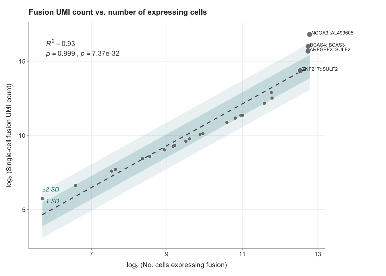
}Single-cell UMI count vs. number of expressing cells (Figure 2D)
A near-perfect correlation between total UMI count and number of expressing cells is expected if probes are working as intended — more expressing cells should yield proportionally more reads. The R² and Spearman ρ values reported here correspond to those in Figure 1D.
# Prepare cleaned labels and flag well-established MCF7 fusions for labelling
stats_clean <- stats %>%
  { if (!"fusion_id" %in% colnames(.)) rownames_to_column(., "fusion_id") else . } %>%
  mutate(
    clean_label = str_extract(fusion_id, "^[^-]+-[^-]+") %>%
      str_replace("-", "::"),
    established = clean_label %in% c(
      "BCAS4::BCAS3", "ARFGEF2::SULF2", "ZNF217::SULF2", "NCOA3::AL499605"
    )
  )

# Linear model and Spearman correlation
m_cells   <- lm(log2(fusion_reads_mcf7) ~ log2(fusions_cell_nums), stats_clean)
intercept <- coef(m_cells)[1]
slope     <- coef(m_cells)[2]
r_sq      <- summary(m_cells)$r.squared
resid_sd  <- sd(residuals(m_cells))

cor_cells <- cor.test(
  stats_clean$fusions_cell_nums,
  stats_clean$fusion_reads_mcf7,
  method = "spearman",
  exact  = FALSE
)

# Ribbon data (±1 and ±2 SD bands)
x_range_c <- range(log2(stats_clean$fusions_cell_nums))
ribbon_c  <- data.frame(x = seq(x_range_c[1], x_range_c[2], length.out = 200)) %>%
  mutate(
    fitted = intercept + slope * x,
    sd1_hi = fitted + 1 * resid_sd,
    sd1_lo = fitted - 1 * resid_sd,
    sd2_hi = fitted + 2 * resid_sd,
    sd2_lo = fitted - 2 * resid_sd
  )

stats_clean <- stats_clean %>%
  mutate(residual_cells = residuals(m_cells))

r_sq_label <- sprintf("italic(R)^2 == %.2f", r_sq)
rho_label  <- sprintf(
  "italic(ρ) == %.3f ~ ',' ~ italic(p) == %.2e",
  cor_cells$estimate,
  cor_cells$p.value
)
x_annot <- x_range_c[1] + 0.1
y_annot <- max(log2(stats_clean$fusion_reads_mcf7))

ggplot(stats_clean,
       aes(x = log2(fusions_cell_nums), y = log2(fusion_reads_mcf7))) +

  geom_ribbon(data = ribbon_c, aes(x = x, ymin = sd2_lo, ymax = sd2_hi),
              fill = "#1A7A8A", alpha = 0.10, inherit.aes = FALSE) +
  geom_ribbon(data = ribbon_c, aes(x = x, ymin = sd1_lo, ymax = sd1_hi),
              fill = "#1A7A8A", alpha = 0.18, inherit.aes = FALSE) +
  geom_line(data = ribbon_c, aes(x = x, y = fitted),
            color = "grey30", linetype = "dashed", linewidth = 0.6, inherit.aes = FALSE) +

  geom_point(aes(size = established),
             shape = 21, fill = "grey40", color = "white", stroke = 0.3, alpha = 0.85) +
  scale_size_manual(values = c("TRUE" = 3, "FALSE" = 2), guide = "none") +

  geom_text(data = stats_clean %>% filter(established), aes(label = clean_label),
            size = 2.25, color = "grey15", hjust = 0, nudge_x = 0.05, nudge_y = 0.12) +

  annotate("text", x = x_range_c[1],
           y = intercept + slope * x_range_c[1] + 1 * resid_sd + 0.15,
           label = "±1 SD", hjust = 0, size = 2.8, color = "#1A7A8A", fontface = "italic") +
  annotate("text", x = x_range_c[1],
           y = intercept + slope * x_range_c[1] + 2 * resid_sd + 0.15,
           label = "±2 SD", hjust = 0, size = 2.8, color = "#1A7A8A", fontface = "italic") +

  annotate("text", x = x_annot, y = y_annot - 0.3,
           label = r_sq_label, parse = TRUE, hjust = 0, vjust = 1, size = 3.2, color = "grey30") +
  annotate("text", x = x_annot, y = y_annot - 1.1,
           label = rho_label, parse = TRUE, hjust = 0, vjust = 1, size = 3.2, color = "grey30") +

  coord_cartesian(clip = "off") +
  labs(
    x     = expression(log[2] ~ "(No. cells expressing fusion)"),
    y     = expression(log[2] ~ "(Single-cell fusion UMI count)"),
    title = "Fusion UMI count vs. number of expressing cells"
  ) +
  theme_classic(base_size = 10) +
  theme(
    plot.title       = element_text(size = 10, face = "bold", color = "grey15", margin = margin(b = 8)),
    plot.margin      = margin(12, 80, 8, 8),
    axis.title       = element_text(size = 9, color = "grey20"),
    axis.title.x     = element_text(margin = margin(t = 6)),
    axis.title.y     = element_text(margin = margin(r = 6)),
    axis.text        = element_text(size = 8, color = "grey30"),
    axis.line        = element_line(color = "grey60", linewidth = 0.4),
    axis.ticks       = element_line(color = "grey60", linewidth = 0.3),
    panel.grid.major = element_line(color = "grey95", linewidth = 0.4),
    panel.grid.minor = element_blank()
  )
| Version | Author | Date |
|---|---|---|
| 1b5bb97 | Jovana Maksimovic | 2026-05-11 |
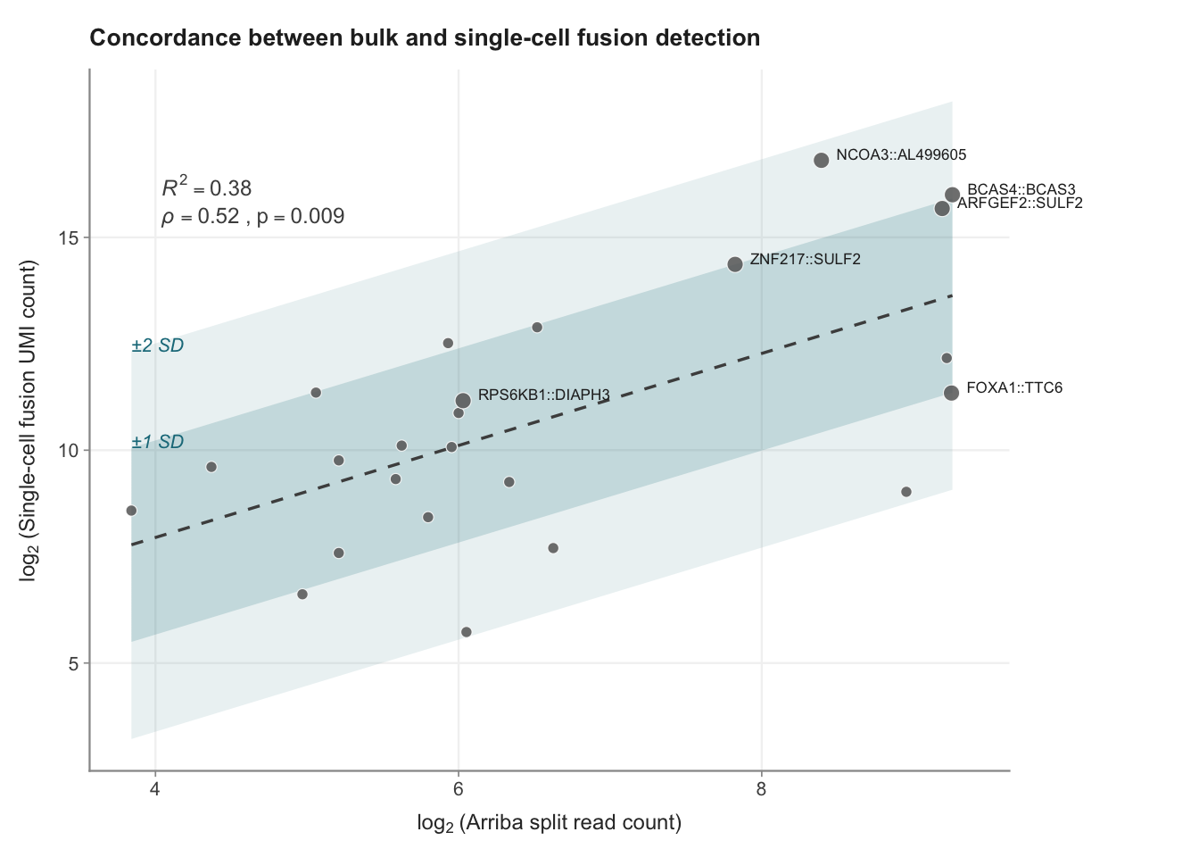
Concordance between bulk (Arriba) and single-cell fusion detection (Figure 2E)
Compares total single-cell UMI counts per fusion to the Arriba split read count from bulk RNA-seq. Higher Spearman ρ indicates better concordance between the two detection methods. The R² and ρ reported here correspond to Figure 1E.
# Prepare cleaned labels; this plot labels 6 established fusions (vs. 4 in Figure 2D above),
# adding RPS6KB1::DIAPH3 and FOXA1::TTC6 which have reliable Arriba support
stats_clean <- stats %>%
  { if (!"fusion_id" %in% colnames(.)) rownames_to_column(., "fusion_id") else . } %>%
  mutate(
    clean_label = str_extract(fusion_id, "^[^-]+-[^-]+") %>%
      str_replace("-", "::"),
    established = clean_label %in% c(
      "BCAS4::BCAS3", "ARFGEF2::SULF2", "ZNF217::SULF2",
      "RPS6KB1::DIAPH3", "FOXA1::TTC6", "NCOA3::AL499605"
    )
  )

# Linear model on log2 scale and Spearman correlation
m         <- lm(log2(fusion_reads_mcf7) ~ log2(average_sum_split_reads), stats_clean)
intercept <- coef(m)[1]
slope     <- coef(m)[2]
r_sq      <- summary(m)$r.squared
resid_sd  <- sd(residuals(m))

cor_result <- cor.test(
  stats_clean$average_sum_split_reads,
  stats_clean$fusion_reads_mcf7,
  method = "spearman",
  exact  = FALSE
)

# Ribbon data
x_range   <- range(log2(stats_clean$average_sum_split_reads))
ribbon_df <- data.frame(x = seq(x_range[1], x_range[2], length.out = 200)) %>%
  mutate(
    fitted = intercept + slope * x,
    sd1_hi = fitted + 1 * resid_sd,
    sd1_lo = fitted - 1 * resid_sd,
    sd2_hi = fitted + 2 * resid_sd,
    sd2_lo = fitted - 2 * resid_sd
  )

stats_clean <- stats_clean %>%
  mutate(residual = residuals(m))

r_sq_label <- sprintf("italic(R)^2 == %.2f", r_sq)
rho_label  <- sprintf(
  "italic(ρ) == %.2f ~ ',' ~ p == %.3f",
  cor_result$estimate,
  cor_result$p.value
)
x_annot <- x_range[1] + 0.2
y_annot <- max(log2(stats_clean$fusion_reads_mcf7))

ggplot(stats_clean,
       aes(x = log2(average_sum_split_reads), y = log2(fusion_reads_mcf7))) +

  geom_ribbon(data = ribbon_df, aes(x = x, ymin = sd2_lo, ymax = sd2_hi),
              fill = "#1A7A8A", alpha = 0.10, inherit.aes = FALSE) +
  geom_ribbon(data = ribbon_df, aes(x = x, ymin = sd1_lo, ymax = sd1_hi),
              fill = "#1A7A8A", alpha = 0.18, inherit.aes = FALSE) +
  geom_line(data = ribbon_df, aes(x = x, y = fitted),
            color = "grey30", linetype = "dashed", linewidth = 0.6, inherit.aes = FALSE) +

  geom_point(aes(size = established),
             shape = 21, fill = "grey40", color = "white", stroke = 0.3, alpha = 0.85) +
  scale_size_manual(values = c("TRUE" = 3, "FALSE" = 2), guide = "none") +

  geom_text(data = stats_clean %>% filter(established), aes(label = clean_label),
            size = 2.25, color = "grey15", hjust = 0, nudge_x = 0.1, nudge_y = 0.15) +

  annotate("text", x = x_range[1],
           y = intercept + slope * x_range[1] + 1 * resid_sd + 0.15,
           label = "±1 SD", hjust = 0, size = 2.8, color = "#1A7A8A", fontface = "italic") +
  annotate("text", x = x_range[1],
           y = intercept + slope * x_range[1] + 2 * resid_sd + 0.15,
           label = "±2 SD", hjust = 0, size = 2.8, color = "#1A7A8A", fontface = "italic") +

  annotate("text", x = x_annot, y = y_annot - 0.3,
           label = r_sq_label, parse = TRUE, hjust = 0, vjust = 1, size = 3.2, color = "grey30") +
  annotate("text", x = x_annot, y = y_annot - 1.1,
           label = rho_label, parse = TRUE, hjust = 0, vjust = 1, size = 3.2, color = "grey30") +

  labs(
    x     = expression(log[2] ~ "(Arriba split read count)"),
    y     = expression(log[2] ~ "(Single-cell fusion UMI count)"),
    title = "Concordance between bulk and single-cell fusion detection"
  ) +
  theme_classic(base_size = 10) +
  coord_cartesian(clip = "off") +
  theme(
    plot.title       = element_text(size = 10, face = "bold", color = "grey15", margin = margin(b = 8)),
    plot.margin      = margin(12, 80, 8, 8),
    axis.title       = element_text(size = 9, color = "grey20"),
    axis.title.x     = element_text(margin = margin(t = 6)),
    axis.title.y     = element_text(margin = margin(r = 6)),
    axis.text        = element_text(size = 8, color = "grey30"),
    axis.line        = element_line(color = "grey60", linewidth = 0.4),
    axis.ticks       = element_line(color = "grey60", linewidth = 0.3),
    panel.grid.major = element_line(color = "grey95", linewidth = 0.4),
    panel.grid.minor = element_blank()
  )
| Version | Author | Date |
|---|---|---|
| 1b5bb97 | Jovana Maksimovic | 2026-05-11 |
Compute the residual of each fusion from the regression line for use in the probe quality plots below.
stats$y_residual <- apply(stats, 1, y_residual, intercept, slope)Probe sequence characteristics
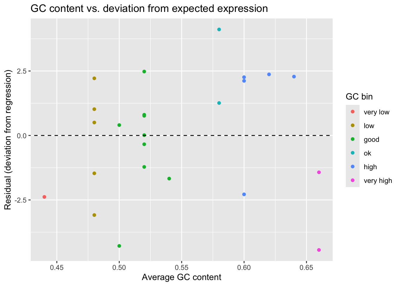
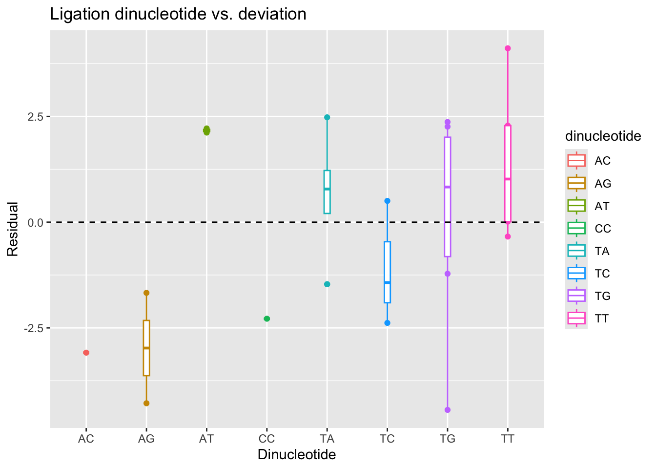
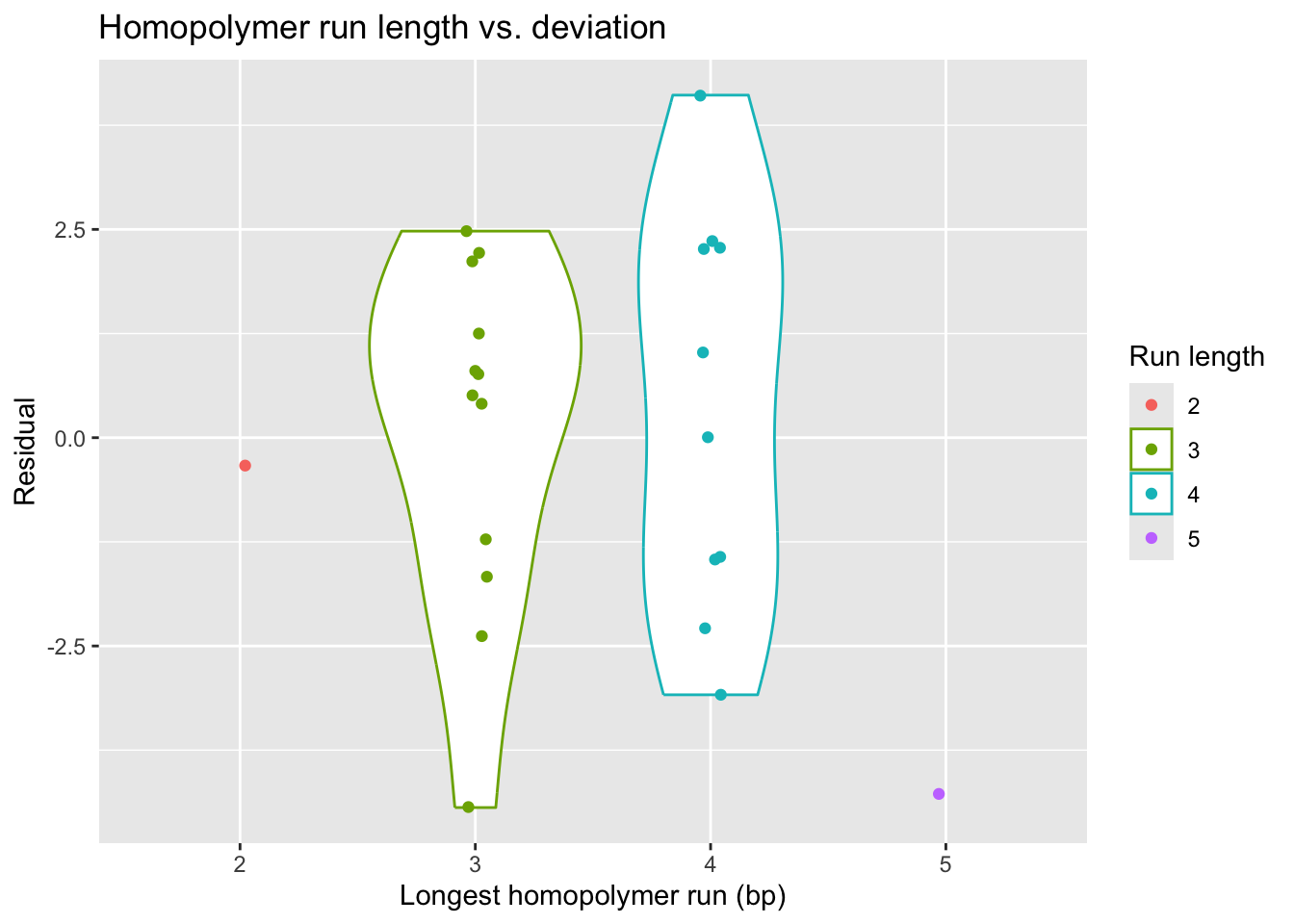
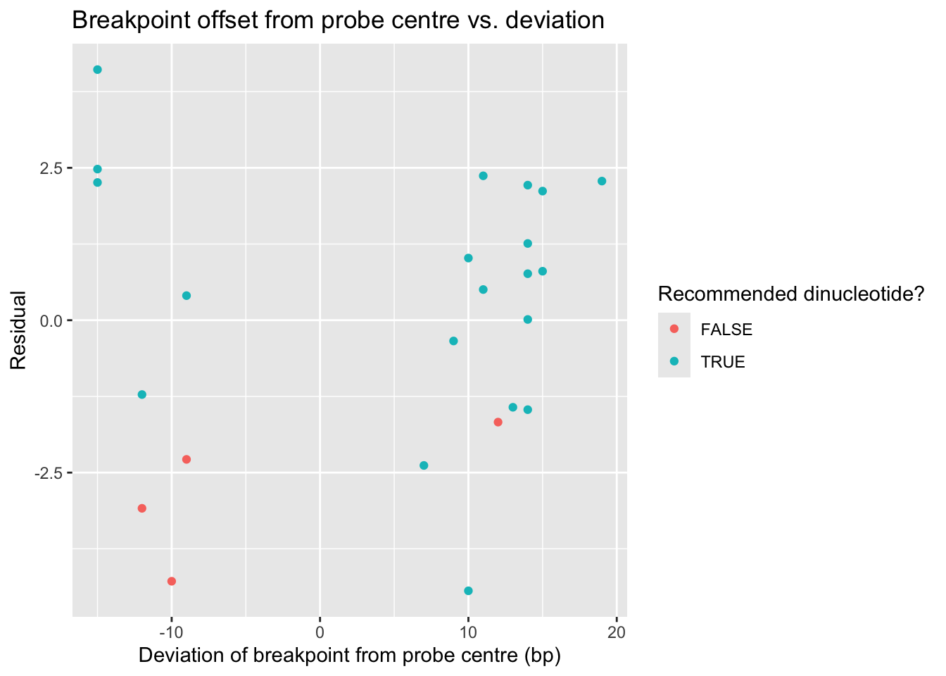
The following analyses examine whether probe sequence properties — GC content, ligation dinucleotide, homopolymer run length, and breakpoint position — are associated with deviation from the expected bulk–single-cell concordance. Greater deviation (positive or negative residual) may suggest the probe is under- or over-performing.
GC content
Average GC content of the two 25 bp probe halves. The 10x recommended range is 44–72%.
stats$average_gc <- (stats$GC_first_half + stats$GC_second_half) / 2
stats$binned_gc  <- unlist(lapply(stats$average_gc, check_gc))
stats$binned_gc  <- with(stats, reorder(binned_gc, average_gc))

ggplot(stats) +
  aes(x = average_gc, y = y_residual, color = binned_gc) +
  geom_point() +
  geom_abline(intercept = 0, slope = 0, color = "black", linetype = "dashed", linewidth = 0.5) +
  labs(
    title = "GC content vs. deviation from expected expression",
    x     = "Average GC content",
    y     = "Residual (deviation from regression)",
    color = "GC bin"
  )
| Version | Author | Date |
|---|---|---|
| 1b5bb97 | Jovana Maksimovic | 2026-05-11 |
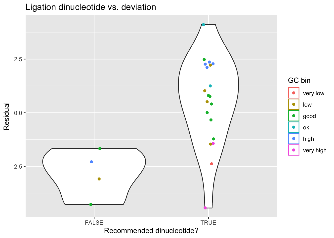
Ligation dinucleotide
Probes are split by whether their ligation junction dinucleotide is in the recommended set. Points are coloured by GC content bin.
ggplot(stats) +
  aes(x = dinucleotide_recommended, y = y_residual,
      group = dinucleotide_recommended, color = binned_gc) +
  geom_violin() +
  geom_point(position = position_jitter(seed = 1, width = 0.05)) +
  labs(
    title = "Ligation dinucleotide vs. deviation",
    x     = "Recommended dinucleotide?",
    y     = "Residual",
    color = "GC bin"
  )
| Version | Author | Date |
|---|---|---|
| 1b5bb97 | Jovana Maksimovic | 2026-05-11 |
ggplot(stats) +
  aes(x = dinucleotide, y = y_residual, color = dinucleotide) +
  geom_point() +
  geom_boxplot(width = 0.1) +
  geom_abline(intercept = 0, slope = 0, color = "black", linetype = "dashed", linewidth = 0.5) +
  labs(
    title = "Ligation dinucleotide vs. deviation",
    x     = "Dinucleotide",
    y     = "Residual"
  )
| Version | Author | Date |
|---|---|---|
| 1b5bb97 | Jovana Maksimovic | 2026-05-11 |
Homopolymer run length
Long homopolymer runs (≥ 4 bp) are penalised in the probe design. Here we check whether probes with longer runs show greater deviation from expected expression.
stats$longest_run_length <- unlist(lapply(stats$Probes, longest_run))

ggplot(stats) +
  aes(x = as.character(longest_run_length), y = y_residual,
      color = as.character(longest_run_length)) +
  geom_violin() +
  geom_point(position = position_jitter(seed = 1, width = 0.05)) +
  labs(
    title = "Homopolymer run length vs. deviation",
    x     = "Longest homopolymer run (bp)",
    y     = "Residual",
    color = "Run length"
  )
| Version | Author | Date |
|---|---|---|
| 1b5bb97 | Jovana Maksimovic | 2026-05-11 |
Breakpoint position within the probe
The ligation breakpoint is nominally at position 25 of the 50 bp probe. Here we examine whether deviation of the breakpoint from the probe centre is associated with performance.
ggplot(stats) +
  aes(x = Deviation_of_break_in_Probe, y = y_residual, color = dinucleotide_recommended) +
  geom_point() +
  labs(
    title = "Breakpoint offset from probe centre vs. deviation",
    x     = "Deviation of breakpoint from probe centre (bp)",
    y     = "Residual",
    color = "Recommended dinucleotide?"
  )
| Version | Author | Date |
|---|---|---|
| 1b5bb97 | Jovana Maksimovic | 2026-05-11 |
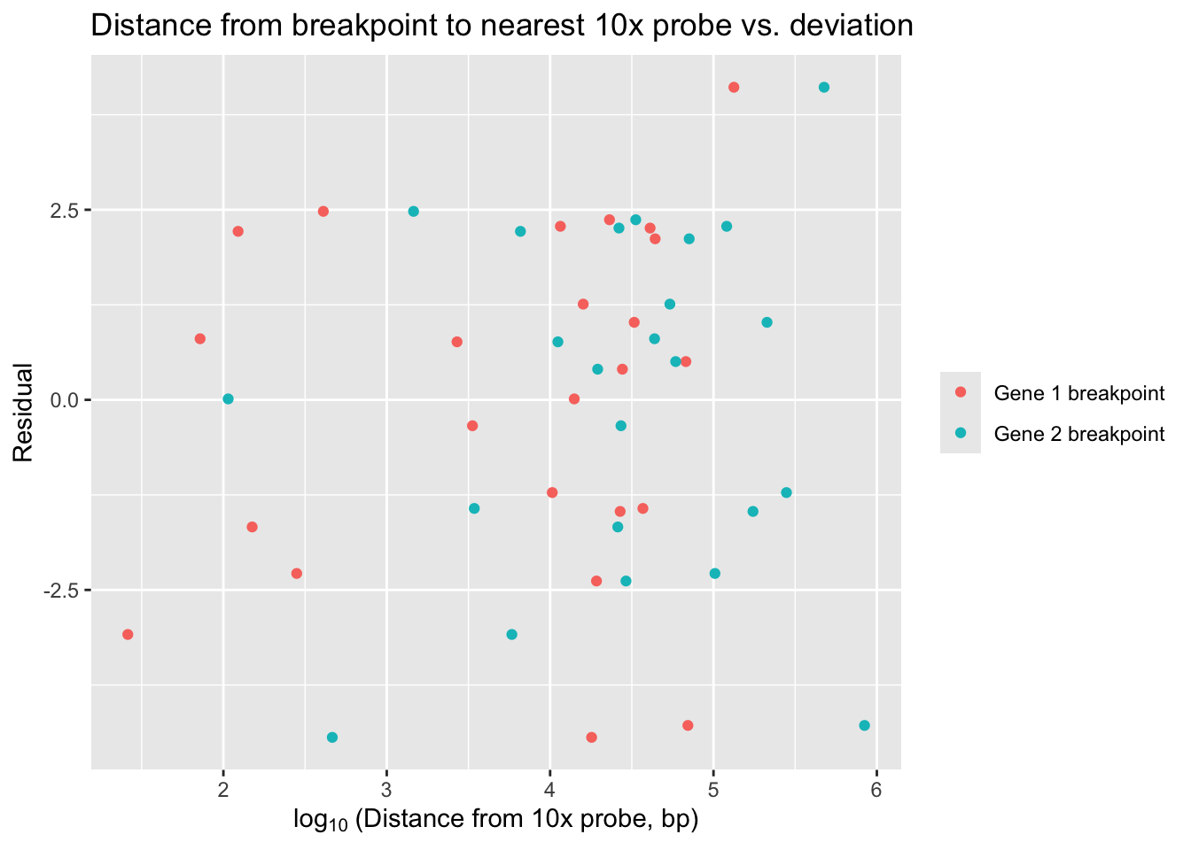
Distance from breakpoint to nearest 10x probe
For each fusion, the distance from each breakpoint to the nearest standard 10x probe in the Chromium Human Transcriptome set. Short distances may increase competition from endogenous probe binding.
ggplot(stats) +
  geom_point(aes(x = log10(fusion1_bp_distance), y = y_residual, color = "Gene 1 breakpoint")) +
  geom_point(aes(x = log10(fusion2_bp_distance), y = y_residual, color = "Gene 2 breakpoint")) +
  labs(
    title  = "Distance from breakpoint to nearest 10x probe vs. deviation",
    x      = expression(log[10] ~ "(Distance from 10x probe, bp)"),
    y      = "Residual",
    color  = NULL
  )
| Version | Author | Date |
|---|---|---|
| 1b5bb97 | Jovana Maksimovic | 2026-05-11 |
Session info
sessioninfo::session_info()─ Session info ───────────────────────────────────────────────────────────────
setting value
version R version 4.4.1 (2024-06-14)
os macOS 15.5
system aarch64, darwin20
ui X11
language (EN)
collate en_US.UTF-8
ctype en_US.UTF-8
tz Australia/Melbourne
date 2026-07-15
pandoc 3.8.3 @ /Applications/RStudio.app/Contents/Resources/app/quarto/bin/tools/aarch64/ (via rmarkdown)
quarto 1.9.38 @ /Applications/RStudio.app/Contents/Resources/app/quarto/bin/quarto
─ Packages ───────────────────────────────────────────────────────────────────
! package * version date (UTC) lib source
P BiocManager 1.30.27 2025-11-14 [?] CRAN (R 4.4.3)
P bslib 0.9.0 2025-01-30 [?] CRAN (R 4.4.1)
P cachem 1.1.0 2024-05-16 [?] CRAN (R 4.4.1)
P callr 3.7.6 2024-03-25 [?] CRAN (R 4.4.0)
P cli 3.6.5 2025-04-23 [?] CRAN (R 4.4.1)
P digest 0.6.37 2024-08-19 [?] CRAN (R 4.4.1)
P dplyr * 1.1.4 2023-11-17 [?] CRAN (R 4.4.0)
P evaluate 1.0.3 2025-01-10 [?] CRAN (R 4.4.1)
P farver 2.1.2 2024-05-13 [?] CRAN (R 4.4.1)
P fastmap 1.2.0 2024-05-15 [?] CRAN (R 4.4.1)
P fs 1.6.6 2025-04-12 [?] CRAN (R 4.4.1)
P generics 0.1.4 2025-05-09 [?] CRAN (R 4.4.1)
P getPass 0.2-4 2023-12-10 [?] CRAN (R 4.4.1)
P ggplot2 * 4.0.2 2026-02-03 [?] CRAN (R 4.4.3)
P git2r 0.36.2 2025-03-29 [?] CRAN (R 4.4.1)
P glue 1.8.0 2024-09-30 [?] CRAN (R 4.4.1)
P gtable 0.3.6 2024-10-25 [?] CRAN (R 4.4.1)
P here * 1.0.1 2020-12-13 [?] CRAN (R 4.4.1)
P htmltools 0.5.8.1 2024-04-04 [?] CRAN (R 4.4.1)
P httpuv 1.6.16 2025-04-16 [?] CRAN (R 4.4.1)
P httr 1.4.7 2023-08-15 [?] CRAN (R 4.4.0)
P jquerylib 0.1.4 2021-04-26 [?] CRAN (R 4.4.0)
P jsonlite 2.0.0 2025-03-27 [?] CRAN (R 4.4.1)
P knitr 1.50 2025-03-16 [?] CRAN (R 4.4.1)
P labeling 0.4.3 2023-08-29 [?] CRAN (R 4.4.1)
P later 1.4.2 2025-04-08 [?] CRAN (R 4.4.1)
P lifecycle 1.0.4 2023-11-07 [?] CRAN (R 4.4.1)
P magrittr 2.0.3 2022-03-30 [?] CRAN (R 4.4.1)
P pillar 1.10.2 2025-04-05 [?] CRAN (R 4.4.1)
P pkgconfig 2.0.3 2019-09-22 [?] CRAN (R 4.4.1)
P processx 3.8.6 2025-02-21 [?] CRAN (R 4.4.1)
P promises 1.3.3 2025-05-29 [?] CRAN (R 4.4.1)
P ps 1.9.1 2025-04-12 [?] CRAN (R 4.4.1)
P R6 2.6.1 2025-02-15 [?] CRAN (R 4.4.1)
P RColorBrewer 1.1-3 2022-04-03 [?] CRAN (R 4.4.1)
P Rcpp 1.1.1-1.1 2026-04-24 [?] CRAN (R 4.4.1)
renv 1.1.4 2025-03-20 [1] CRAN (R 4.4.1)
P rlang 1.1.6 2025-04-11 [?] CRAN (R 4.4.1)
P rmarkdown 2.29 2024-11-04 [?] CRAN (R 4.4.1)
P rprojroot 2.0.4 2023-11-05 [?] CRAN (R 4.4.1)
P rstudioapi 0.17.1 2024-10-22 [?] CRAN (R 4.4.1)
P S7 0.2.0 2024-11-07 [?] CRAN (R 4.4.1)
P sass 0.4.10 2025-04-11 [?] CRAN (R 4.4.1)
P scales 1.4.0 2025-04-24 [?] CRAN (R 4.4.1)
P sessioninfo 1.2.3 2025-02-05 [?] CRAN (R 4.4.1)
P stringi 1.8.7 2025-03-27 [?] CRAN (R 4.4.1)
P stringr * 1.6.0 2025-11-04 [?] CRAN (R 4.4.1)
P tibble * 3.2.1 2023-03-20 [?] CRAN (R 4.4.0)
P tidyselect 1.2.1 2024-03-11 [?] CRAN (R 4.4.0)
P vctrs 0.6.5 2023-12-01 [?] CRAN (R 4.4.0)
P whisker 0.4.1 2022-12-05 [?] CRAN (R 4.4.1)
P withr 3.0.2 2024-10-28 [?] CRAN (R 4.4.1)
P workflowr * 1.7.1 2023-08-23 [?] CRAN (R 4.4.0)
P xfun 0.56 2026-01-18 [?] CRAN (R 4.4.3)
P yaml 2.3.10 2024-07-26 [?] CRAN (R 4.4.1)
[1] /Users/maksimovicjovana/Library/CloudStorage/OneDrive-PeterMac/Desktop/projects/my_research/flex-fusion-probes/renv/library/macos/R-4.4/aarch64-apple-darwin20
[2] /Users/maksimovicjovana/Library/Caches/org.R-project.R/R/renv/sandbox/macos/R-4.4/aarch64-apple-darwin20/f7156815
* ── Packages attached to the search path.
P ── Loaded and on-disk path mismatch.
──────────────────────────────────────────────────────────────────────────────
sessionInfo()R version 4.4.1 (2024-06-14)
Platform: aarch64-apple-darwin20
Running under: macOS 15.5
Matrix products: default
BLAS: /Library/Frameworks/R.framework/Versions/4.4-arm64/Resources/lib/libRblas.0.dylib
LAPACK: /Library/Frameworks/R.framework/Versions/4.4-arm64/Resources/lib/libRlapack.dylib; LAPACK version 3.12.0
locale:
[1] en_US.UTF-8/en_US.UTF-8/en_US.UTF-8/C/en_US.UTF-8/en_US.UTF-8
time zone: Australia/Melbourne
tzcode source: internal
attached base packages:
[1] stats graphics grDevices datasets utils methods base
other attached packages:
[1] tibble_3.2.1 stringr_1.6.0 ggplot2_4.0.2 here_1.0.1
[5] dplyr_1.1.4 workflowr_1.7.1
loaded via a namespace (and not attached):
[1] gtable_0.3.6 jsonlite_2.0.0 compiler_4.4.1
[4] BiocManager_1.30.27 renv_1.1.4 promises_1.3.3
[7] tidyselect_1.2.1 Rcpp_1.1.1-1.1 git2r_0.36.2
[10] callr_3.7.6 later_1.4.2 jquerylib_0.1.4
[13] scales_1.4.0 yaml_2.3.10 fastmap_1.2.0
[16] R6_2.6.1 labeling_0.4.3 generics_0.1.4
[19] knitr_1.50 rprojroot_2.0.4 RColorBrewer_1.1-3
[22] bslib_0.9.0 pillar_1.10.2 rlang_1.1.6
[25] cachem_1.1.0 stringi_1.8.7 httpuv_1.6.16
[28] xfun_0.56 S7_0.2.0 getPass_0.2-4
[31] fs_1.6.6 sass_0.4.10 cli_3.6.5
[34] withr_3.0.2 magrittr_2.0.3 ps_1.9.1
[37] grid_4.4.1 digest_0.6.37 processx_3.8.6
[40] rstudioapi_0.17.1 lifecycle_1.0.4 vctrs_0.6.5
[43] evaluate_1.0.3 glue_1.8.0 farver_2.1.2
[46] whisker_0.4.1 sessioninfo_1.2.3 rmarkdown_2.29
[49] httr_1.4.7 tools_4.4.1 pkgconfig_2.0.3
[52] htmltools_0.5.8.1