Demultiplexing the C133_Neeland_batch2 data set
Peter Hickey and Jovana Maksimovic
2024-02-26
Last updated: 2024-02-26
Checks: 7 0
Knit directory: paed-inflammation-CITEseq/
This reproducible R Markdown analysis was created with workflowr (version 1.7.1). The Checks tab describes the reproducibility checks that were applied when the results were created. The Past versions tab lists the development history.
Great! Since the R Markdown file has been committed to the Git repository, you know the exact version of the code that produced these results.
Great job! The global environment was empty. Objects defined in the global environment can affect the analysis in your R Markdown file in unknown ways. For reproduciblity it’s best to always run the code in an empty environment.
The command set.seed(20240216) was run prior to running
the code in the R Markdown file. Setting a seed ensures that any results
that rely on randomness, e.g. subsampling or permutations, are
reproducible.
Great job! Recording the operating system, R version, and package versions is critical for reproducibility.
Nice! There were no cached chunks for this analysis, so you can be confident that you successfully produced the results during this run.
Great job! Using relative paths to the files within your workflowr project makes it easier to run your code on other machines.
Great! You are using Git for version control. Tracking code development and connecting the code version to the results is critical for reproducibility.
The results in this page were generated with repository version 025ceae. See the Past versions tab to see a history of the changes made to the R Markdown and HTML files.
Note that you need to be careful to ensure that all relevant files for
the analysis have been committed to Git prior to generating the results
(you can use wflow_publish or
wflow_git_commit). workflowr only checks the R Markdown
file, but you know if there are other scripts or data files that it
depends on. Below is the status of the Git repository when the results
were generated:
Ignored files:
    Ignored:    .Rhistory
    Ignored:    .Rproj.user/

Untracked files:
    Untracked:  .DS_Store
    Untracked:  analysis/02.0_quality_control.Rmd
    Untracked:  analysis/03.0_call_doublets.Rmd
    Untracked:  code/dropletutils.R
    Untracked:  code/utility.R
    Untracked:  data/.DS_Store
    Untracked:  data/C133_Neeland_batch0/
    Untracked:  data/C133_Neeland_batch1/
    Untracked:  data/C133_Neeland_batch2/
    Untracked:  data/C133_Neeland_batch3/
    Untracked:  data/C133_Neeland_batch4/
    Untracked:  data/C133_Neeland_batch5/
    Untracked:  data/C133_Neeland_batch6/
    Untracked:  renv.lock
    Untracked:  renv/

Unstaged changes:
    Modified:   .Rprofile
    Modified:   .gitignore
Note that any generated files, e.g. HTML, png, CSS, etc., are not included in this status report because it is ok for generated content to have uncommitted changes.
These are the previous versions of the repository in which changes were
made to the R Markdown
(analysis/01.2_preprocess_batch2.Rmd) and HTML
(docs/01.2_preprocess_batch2.html) files. If you’ve
configured a remote Git repository (see ?wflow_git_remote),
click on the hyperlinks in the table below to view the files as they
were in that past version.
| File | Version | Author | Date | Message |
|---|---|---|---|---|
| Rmd | 025ceae | Jovana Maksimovic | 2024-02-26 | wflow_publish(c("analysis/index.Rmd", "analysis/01*")) |
suppressPackageStartupMessages({
    library(here)
    library(readxl)
    library(BiocStyle)
    library(ggplot2)
    library(cowplot)
    library(patchwork)
    library(demuxmix)
    library(tidyverse)
    library(SingleCellExperiment)
    library(DropletUtils)
    library(scater)
})

source(here("code/utility.R"))
Overview
- There are 8 samples in this batch.
- Each sample comes from a different donor (i.e. each sample is genetically distinct).
- Each has a unique HTO label.
We used simple HTO labelling whereby each sample is labelled with 1 HTO, shown in the table below:
sample_metadata_df <- read_excel(
  here("data/C133_Neeland_batch2/data/sample_sheets/CITEseq_48 samples_design_2.xlsx"),
  col_types =
    c("text", "text", "text", "numeric", "text", "numeric", "text", "date"))
sample_metadata_df$`HASHTAG ID` <- paste0(
  "Human_HTO_",
  sample_metadata_df$`HASHTAG ID`)
knitr::kable(sample_metadata_df[sample_metadata_df$Batch == 2, ])| Donor | Sample name | Disease | Age | Sex | Batch | HASHTAG ID | DATE OF CAPTURE |
|---|---|---|---|---|---|---|---|
| 9 | 9 | Wheeze | 3.665753 | M | 2 | Human_HTO_6 | 2021-09-06 |
| 10 | 10 | True control | 8.397260 | F | 2 | Human_HTO_7 | 2021-09-06 |
| 11 | 11.1 | CF | 2.947945 | F | 2 | Human_HTO_9 | 2021-09-06 |
| 11 | 11.2 | CF | 4.572603 | F | 2 | Human_HTO_10 | 2021-09-06 |
| 11 | 11.3 | CF | 4.917808 | F | 2 | Human_HTO_12 | 2021-09-06 |
| 12 | 12.1 | CF | 2.969863 | M | 2 | Human_HTO_13 | 2021-09-06 |
| 12 | 12.2 | CF | 4.057534 | M | 2 | Human_HTO_14 | 2021-09-06 |
| 12 | 12.3 | CF | 5.093151 | M | 2 | Human_HTO_15 | 2021-09-06 |
Setting up the data
sce_raw <- readRDS(here("data", "C133_Neeland_batch2",
                    "data", "SCEs", "C133_Neeland_batch2.CellRanger.SCE.rds"))
sce_raw$Capture <- factor(sce_raw$Sample)
capture_names <- levels(sce_raw$Capture)
capture_names <- setNames(capture_names, capture_names)
sce_raw$Sample <- NULL
sce_raw
class: SingleCellExperiment
dim: 36601 6612251
metadata(1): Samples
assays(1): counts
rownames(36601): ENSG00000243485 ENSG00000237613 ... ENSG00000278817
ENSG00000277196
rowData names(3): ID Symbol Type
colnames(6612251): 1_AAACCCAAGAAACACT-1 1_AAACCCAAGAAACCAT-1 ...
2_TTTGTTGTCTTTGCAT-1 2_TTTGTTGTCTTTGGAG-1
colData names(2): Barcode Capture
reducedDimNames(0):
mainExpName: Gene Expression
altExpNames(1): Antibody CaptureCalling cells from empty droplets
par(mfrow = c(1, 2))
lapply(capture_names, function(cn) {
  sce_raw <- sce_raw[, sce_raw$Capture == cn]
  bcrank <- barcodeRanks(counts(sce_raw))
  # Only showing unique points for plotting speed.
  uniq <- !duplicated(bcrank$rank)
  plot(
    x = bcrank$rank[uniq],
    y = bcrank$total[uniq],
    log = "xy",
    xlab = "Rank",
    ylab = "Total UMI count",
    main = cn,
    cex.lab = 1.2,
    xlim = c(1, 500000),
    ylim = c(1, 200000))
  abline(h = metadata(bcrank)$inflection, col = "darkgreen", lty = 2)
  abline(h = metadata(bcrank)$knee, col = "dodgerblue", lty = 2)
})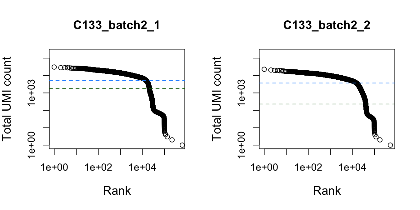
Total UMI count for each barcode in the dataset, plotted against its rank (in decreasing order of total counts). The inferred locations of the inflection (dark green dashed lines) and knee points (blue dashed lines) are also shown.
Remove empty droplets.
empties <- do.call(rbind, lapply(capture_names, function(cn) {
  message(cn)
  empties <- readRDS(
    here("data",
         "C133_Neeland_batch2",
         "data",
         "emptyDrops", paste0(cn, ".emptyDrops.rds")))
  empties$Capture <- cn
  empties
}))
tapply(
  empties$FDR,
  empties$Capture,
  function(x) sum(x <= 0.001, na.rm = TRUE)) |>
  knitr::kable(
caption = "Number of non-empty droplets identified using `emptyDrops()` from **DropletUtils**.")| x | |
|---|---|
| C133_batch2_1 | 23753 |
| C133_batch2_2 | 29407 |
sce <- sce_raw[, which(empties$FDR <= 0.001)]
sce
class: SingleCellExperiment
dim: 36601 53160
metadata(1): Samples
assays(1): counts
rownames(36601): ENSG00000243485 ENSG00000237613 ... ENSG00000278817
ENSG00000277196
rowData names(3): ID Symbol Type
colnames(53160): 1_AAACCCAAGACCTGGA-1 1_AAACCCAAGACTGTTC-1 ...
2_TTTGTTGTCTCATGGA-1 2_TTTGTTGTCTCCAAGA-1
colData names(2): Barcode Capture
reducedDimNames(0):
mainExpName: Gene Expression
altExpNames(1): Antibody CaptureAdding per cell quality control information
sce <- scuttle::addPerCellQC(sce)
head(colData(sce)) %>%
  data.frame %>%
knitr::kable()| Barcode | Capture | sum | detected | altexps_Antibody.Capture_sum | altexps_Antibody.Capture_detected | altexps_Antibody.Capture_percent | total | |
|---|---|---|---|---|---|---|---|---|
| 1_AAACCCAAGACCTGGA-1 | AAACCCAAGACCTGGA-1 | C133_batch2_1 | 7891 | 2571 | 2715 | 154 | 25.59872 | 10606 |
| 1_AAACCCAAGACTGTTC-1 | AAACCCAAGACTGTTC-1 | C133_batch2_1 | 6160 | 2035 | 9563 | 167 | 60.82173 | 15723 |
| 1_AAACCCAAGAGCCATG-1 | AAACCCAAGAGCCATG-1 | C133_batch2_1 | 5190 | 1919 | 2424 | 159 | 31.83609 | 7614 |
| 1_AAACCCAAGAGGACTC-1 | AAACCCAAGAGGACTC-1 | C133_batch2_1 | 8594 | 2746 | 10553 | 163 | 55.11568 | 19147 |
| 1_AAACCCAAGATGATTG-1 | AAACCCAAGATGATTG-1 | C133_batch2_1 | 6089 | 2217 | 3779 | 159 | 38.29550 | 9868 |
| 1_AAACCCAAGCGCACAA-1 | AAACCCAAGCGCACAA-1 | C133_batch2_1 | 3273 | 1406 | 1976 | 160 | 37.64527 | 5249 |
Demultiplexing with hashtag oligos (HTOs)
is_adt <- grepl("^A[0-9]+", rownames(altExp(sce, "Antibody Capture")))
is_hto <- grepl("^Human_HTO", rownames(altExp(sce, "Antibody Capture")))
altExp(sce, "HTO") <- altExp(sce, "Antibody Capture")[is_hto, ]
altExp(sce, "ADT") <- altExp(sce, "Antibody Capture")[is_adt, ]
altExp(sce, "Antibody Capture") <- NULL
hto_counts <- counts(altExp(sce, "HTO"))
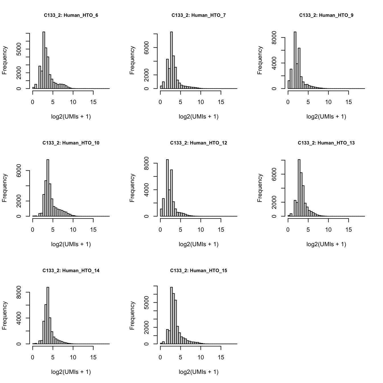
xmax <- ceiling(max(log2(hto_counts + 1)))C133_batch2_1
par(mfrow = c(3, 3))
lapply(rownames(hto_counts), function(i) {
  hist(
    log2(hto_counts[i, sce$Capture == "C133_batch2_1"] + 1),
    xlab = "log2(UMIs + 1)",
    main = paste0("C133_1: ", i),
    xlim = c(0, xmax),
    breaks = seq(0, xmax, 0.5),
    cex.main = 0.8)
})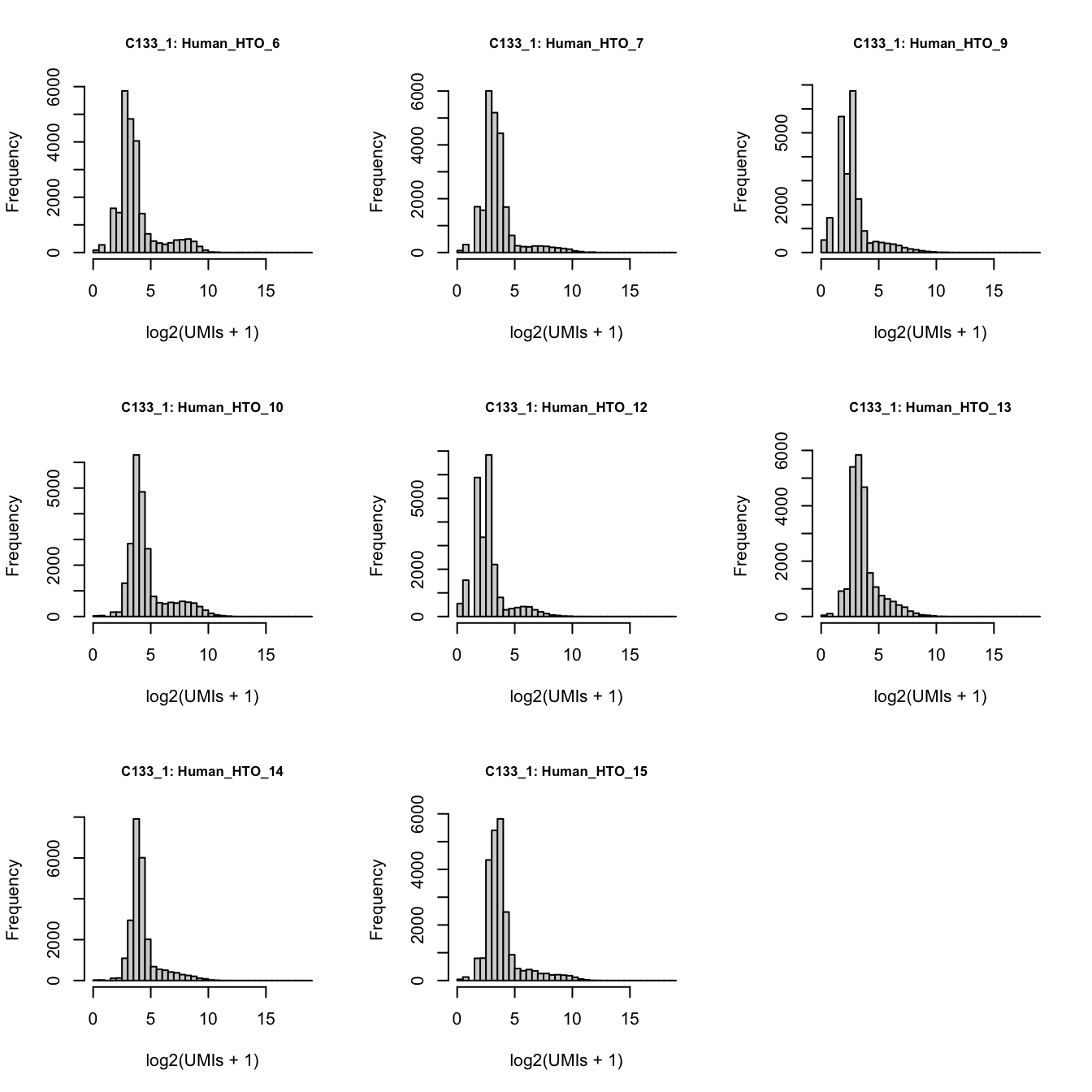
Number of UMIs for each HTO across all non-empty droplets.
Prepare the data.
hto <- as.matrix(counts(altExp(sce[, sce$Capture == "C133_batch2_1"], "HTO")))
detected <- sce$detected[sce$Capture == "C133_batch2_1"]

df <- data.frame(t(hto),
                 detected = detected,
                 hto = colSums(hto))

df %>%
  pivot_longer(cols = starts_with("Human_HTO")) %>%
  mutate(logged = log(value + 1)) %>%
  ggplot(aes(x = logged)) +
  geom_density(adjust = 5) +
  facet_wrap(~name, scales = "free")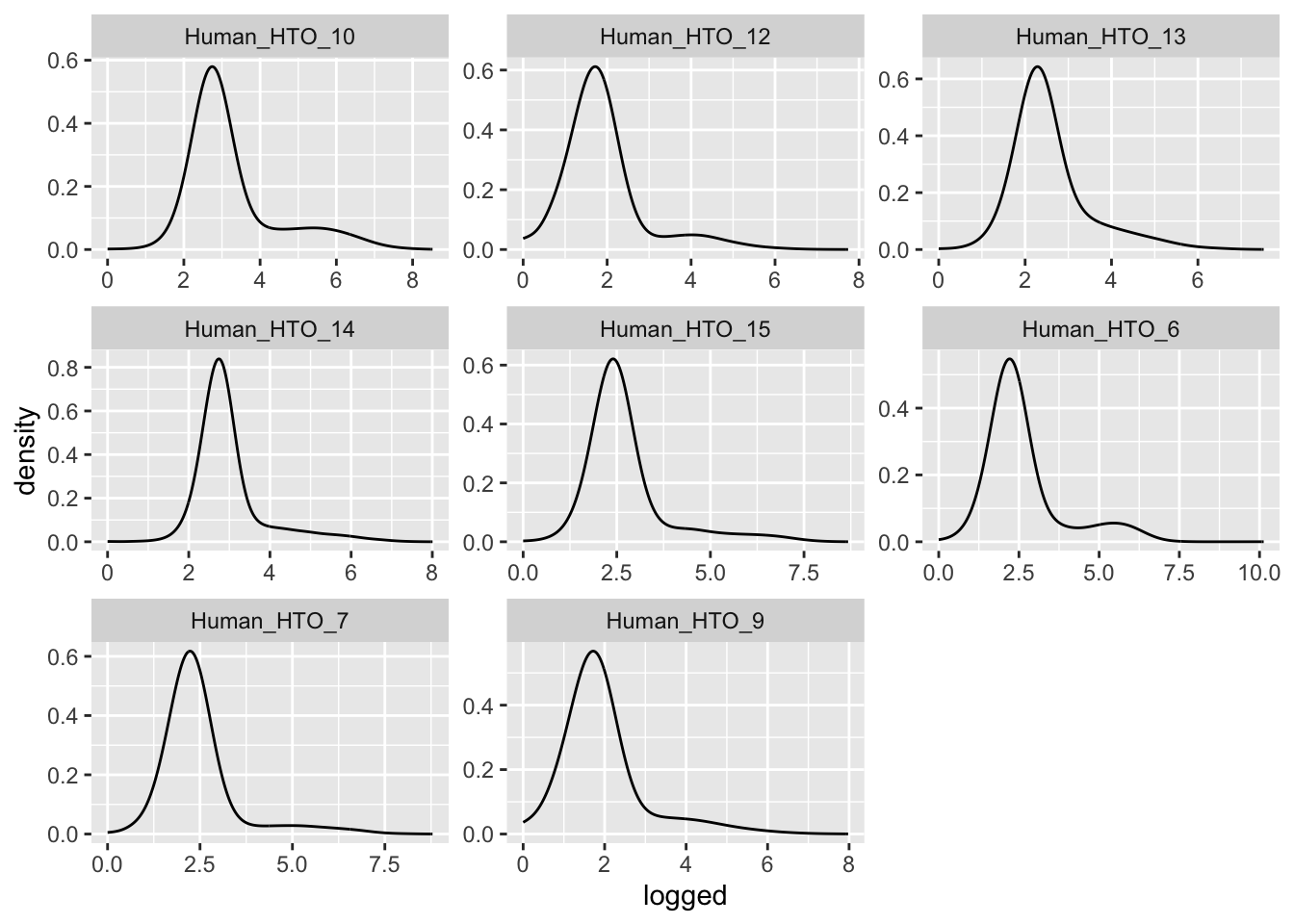
df %>%
  pivot_longer(cols = starts_with("Human_HTO")) %>%
  ggplot(aes(x = detected, y = hto)) +
  geom_density_2d() +
facet_wrap(~name) 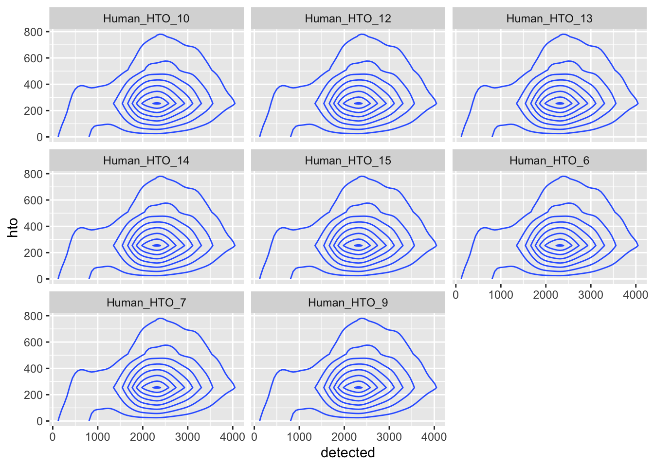
Run demultiplexing.
dmm <- demuxmix(hto = hto,
                rna = detected,
                model = "naive")
summary(dmm)
Class NumObs RelFreq MedProb ExpFPs FDR
1 Human_HTO_10 2866 0.12742308 0.7904544 705.2727 0.2460826
2 Human_HTO_12 1452 0.06455629 0.7769471 369.3228 0.2543545
3 Human_HTO_13 2378 0.10572648 0.8074798 564.1196 0.2372244
4 Human_HTO_14 1895 0.08425218 0.7970796 460.2876 0.2428958
5 Human_HTO_15 1527 0.06789081 0.7895507 375.2009 0.2457111
6 Human_HTO_6 1947 0.08656411 0.7746205 505.1135 0.2594317
7 Human_HTO_7 1071 0.04761693 0.7772905 275.3354 0.2570826
8 Human_HTO_9 1711 0.07607149 0.7996587 408.6939 0.2388626
9 singlet 14847 0.66010137 0.7890803 3663.3464 0.2467398
10 multiplet 4829 0.21469856 0.7580791 1355.1782 0.2806333
11 negative 2816 0.12520007 0.7051019 909.5577 0.3229963
12 uncertain 1261 NA NA NA NAExamine results.
p <- vector("list", nrow(hto))
for(i in 1:nrow(hto)){
  p[[i]] <- plotDmmHistogram(dmm, hto = i) +
    coord_cartesian(ylim = c(0, 0.001),
                    xlim = c(-50, 1000)) +
    theme(axis.title = element_text(size = 8),
          axis.text = element_text(size = 6))
}

wrap_plots(p , ncol = 3) 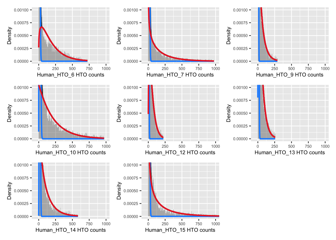
p <- vector("list", nrow(hto))
for(i in 1:nrow(hto)){
  p[[i]] <- plotDmmPosteriorP(dmm, hto = i) +
    theme(axis.title = element_text(size = 8),
          axis.text = element_text(size = 6))
}

wrap_plots(p , ncol = 3) 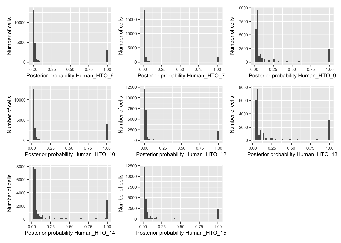
pAcpt(dmm) <- 0
classes1 <- dmmClassify(dmm)
classes1$dmmHTO <- ifelse(classes1$Type == "multiplet", "Doublet",
                           ifelse(classes1$Type %in% c("negative", "uncertain"),
                                  "Negative", classes1$HTO))
table(classes1$dmmHTO)
     Doublet Human_HTO_10 Human_HTO_12 Human_HTO_13 Human_HTO_14 Human_HTO_15
        5420         2917         1491         2434         1935         1564
 Human_HTO_6  Human_HTO_7  Human_HTO_9     Negative
        2019         1117         1769         3087
C133_batch2_2
par(mfrow = c(3, 3))
lapply(rownames(hto_counts), function(i) {
  hist(
    log2(hto_counts[i, sce$Capture == "C133_batch2_2"] + 1),
    xlab = "log2(UMIs + 1)",
    main = paste0("C133_2: ", i),
    xlim = c(0, xmax),
    breaks = seq(0, xmax, 0.5),
    cex.main = 0.8)
})
Number of UMIs for each HTO across all non-empty droplets.
Prepare the data.
hto <- as.matrix(counts(altExp(sce[, sce$Capture == "C133_batch2_2"], "HTO")))
detected <- sce$detected[sce$Capture == "C133_batch2_2"]

df <- data.frame(t(hto),
                 detected = detected,
                 hto = colSums(hto))

df %>%
  pivot_longer(cols = starts_with("Human_HTO")) %>%
  mutate(logged = log(value + 1)) %>%
  ggplot(aes(x = logged)) +
  geom_density(adjust = 5) +
  facet_wrap(~name, scales = "free")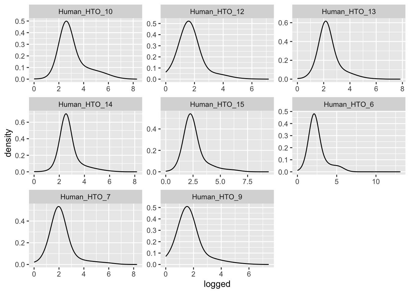
df %>%
  pivot_longer(cols = starts_with("Human_HTO")) %>%
  ggplot(aes(x = detected, y = hto)) +
  geom_density_2d() +
facet_wrap(~name) 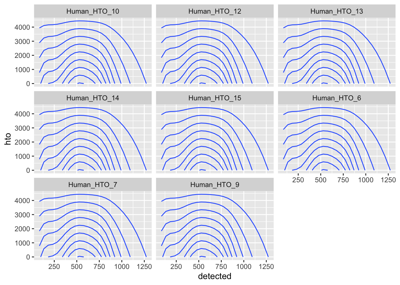
Run demultiplexing.
dmm <- demuxmix(hto = hto,
                rna = detected,
                model = "naive")
summary(dmm)
Class NumObs RelFreq MedProb ExpFPs FDR
1 Human_HTO_10 2904 0.12348514 0.6646074 1041.6423 0.3586922
2 Human_HTO_12 1376 0.05851086 0.6396228 522.7114 0.3798775
3 Human_HTO_13 1860 0.07909172 0.6550031 684.6002 0.3680646
4 Human_HTO_14 1653 0.07028958 0.6551081 603.1705 0.3648945
5 Human_HTO_15 1535 0.06527193 0.6626550 557.3451 0.3630913
6 Human_HTO_6 1837 0.07811370 0.6518793 679.4484 0.3698685
7 Human_HTO_7 1059 0.04503125 0.6447616 397.6371 0.3754835
8 Human_HTO_9 1487 0.06323085 0.6657127 533.7296 0.3589304
9 singlet 13711 0.58302505 0.6558067 5020.2847 0.3661501
10 multiplet 5104 0.21703449 0.6455794 1877.2924 0.3678081
11 negative 4702 0.19994047 0.5881868 1979.1232 0.4209109
12 uncertain 5890 NA NA NA NAExamine results.
p <- vector("list", nrow(hto))
for(i in 1:nrow(hto)){
  p[[i]] <- plotDmmHistogram(dmm, hto = i) +
    coord_cartesian(ylim = c(0, 0.001),
                    xlim = c(-50, 1000)) +
    theme(axis.title = element_text(size = 8),
          axis.text = element_text(size = 6))
}

wrap_plots(p , ncol = 3) 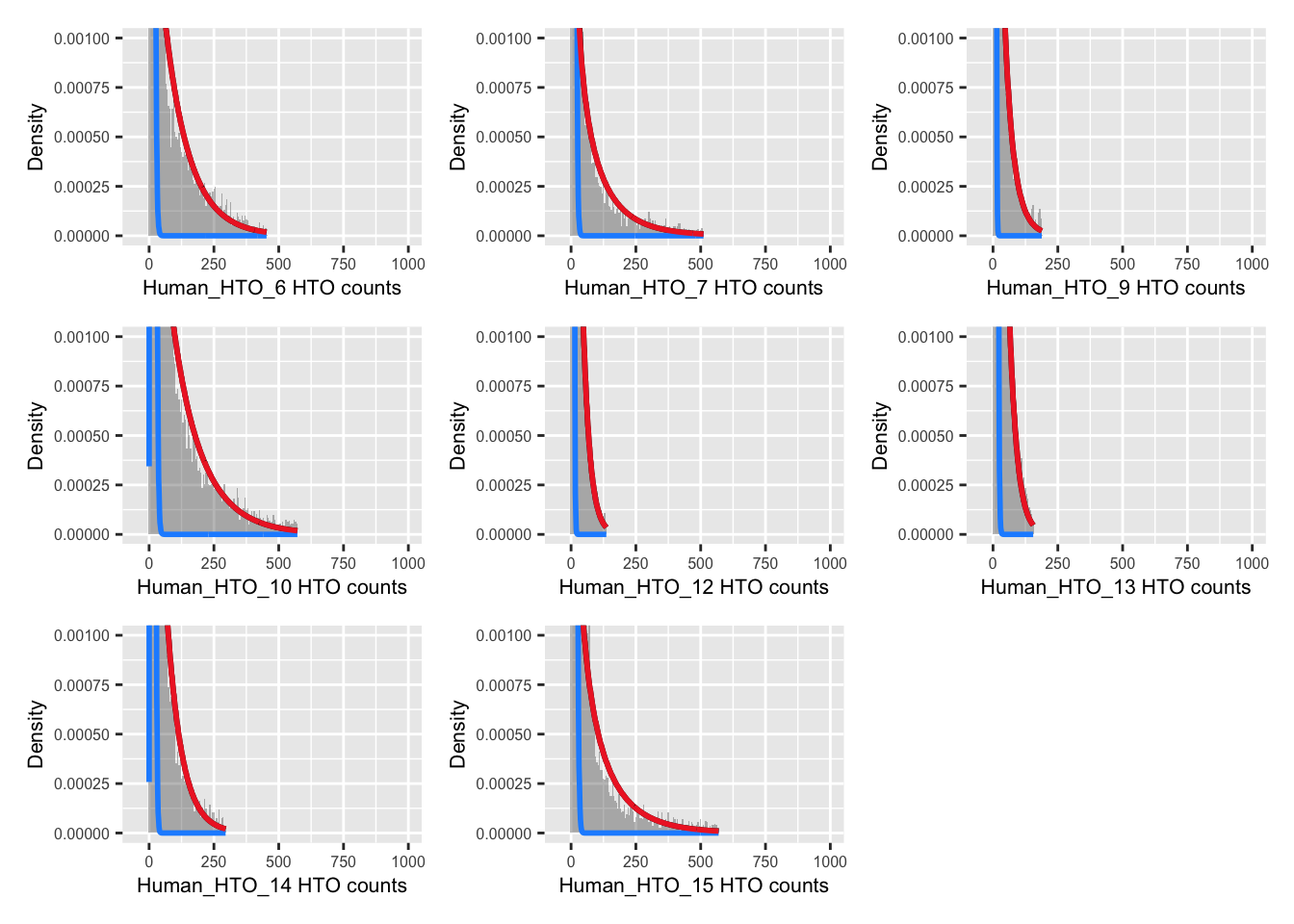
p <- vector("list", nrow(hto))
for(i in 1:nrow(hto)){
  p[[i]] <- plotDmmPosteriorP(dmm, hto = i) +
    theme(axis.title = element_text(size = 8),
          axis.text = element_text(size = 6))
}

wrap_plots(p , ncol = 3) 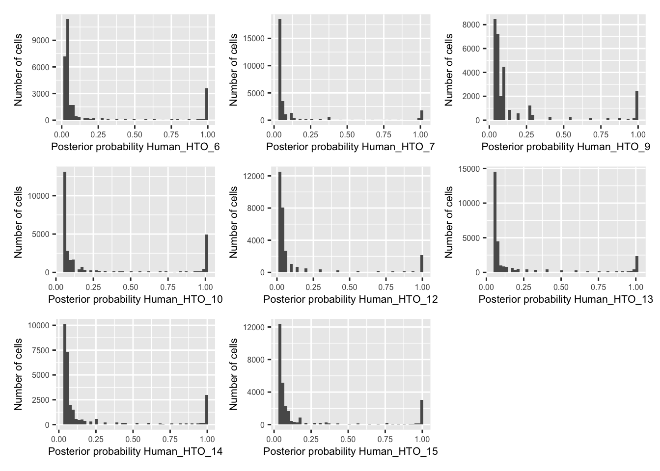
pAcpt(dmm) <- 0
classes2 <- dmmClassify(dmm)
classes2$dmmHTO <- ifelse(classes2$Type == "multiplet", "Doublet",
                           ifelse(classes2$Type %in% c("negative", "uncertain"),
                                  "Negative", classes2$HTO))
table(classes2$dmmHTO)
     Doublet Human_HTO_10 Human_HTO_12 Human_HTO_13 Human_HTO_14 Human_HTO_15
        7715         3269         1552         2179         1895         1777
 Human_HTO_6  Human_HTO_7  Human_HTO_9     Negative
        2123         1210         1665         6022
Save HTO assignments
classes <- rbind(classes1, classes2)
all(rownames(classes) == colnames(sce))
[1] TRUEsce$dmmHTO <- factor(classes$dmmHTO,
levels = c(sort(unique(grep("Human",
classes$dmmHTO,
value = TRUE))),
"Doublet",
"Negative"))Demultiplexing cells without genotype reference
Matching donors across captures
library(vcfR)
f <- sapply(capture_names, function(cn) {
  here("data",
       "C133_Neeland_batch2",
       "data",
       "vireo", cn, "GT_donors.vireo.vcf.gz")
})
x <- lapply(f, read.vcfR, verbose = FALSE)
# Create unique ID for each locus in each capture.
y <- lapply(x, function(xx) {
  paste(
  xx@fix[,"CHROM"],
  xx@fix[,"POS"],
  xx@fix[,"REF"],
  xx@fix[,"ALT"],
  sep = "_")
})
# Only keep the loci in common between the 2 captures.
i <- lapply(y, function(yy) {
  na.omit(match(Reduce(intersect, y), yy))
})
# Construct genotype matrix at common loci from the 2 captures.
donor_names <- paste0("donor", 0:3)
g <- mapply(
  function(xx, ii) {
    apply(
      xx@gt[ii, donor_names],
      2,
      function(x) sapply(strsplit(x, ":"), `[[`, 1))
  },
  xx = x,
  ii = i,
  SIMPLIFY = FALSE)
# Count number of genotype matches between pairs of donors (one from each
# capture) and convert to a proportion.
z <- lapply(2:length(capture_names), function(k) {
  zz <- matrix(
    NA_real_,
    nrow = length(donor_names),
    ncol = length(donor_names),
    dimnames = list(donor_names, donor_names))
  for (ii in rownames(zz)) {
    for (jj in colnames(zz)) {
      zz[ii, jj] <- sum(g[[1]][, ii] == g[[k]][, jj]) / nrow(g[[1]])
    }
  }
  zz
})
heatmaps <- lapply(seq_along(z), function(k) {
pheatmap::pheatmap(
z[[k]],
color = viridisLite::inferno(101),
cluster_rows = FALSE,
cluster_cols = FALSE,
main = "Proportion of matching genotypes",
display_numbers = TRUE,
number_color = "grey50",
labels_row = paste0("C133_batch2_1: ", rownames(z[[k]])),
labels_col = paste0("C133_batch2_", k + 1, ": ", colnames(z[[k]])),
silent = TRUE,
fontsize = 10)
})
gridExtra::grid.arrange(grobs = lapply(heatmaps, `[[`, "gtable"), ncol = 1)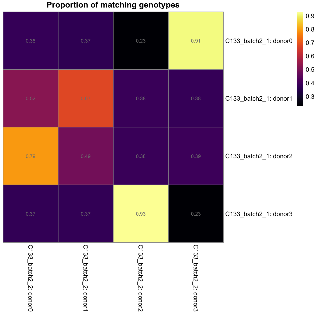
Proportion of matching genotypes between pairs of captures.
The table below gives the best matches between the captures.
best_match_df <- data.frame(
  c(
    list(rownames(z[[1]])),
    lapply(seq_along(z), function(k) {
      apply(
        z[[k]],
        1,
        function(x) colnames(z[[k]])[which.max(x)])
    })),
  row.names = NULL)
colnames(best_match_df) <- capture_names
best_match_df$GeneticDonor <- LETTERS[seq_along(donor_names)]
best_match_df <- dplyr::select(best_match_df, GeneticDonor, everything())

knitr::kable(
  best_match_df,
caption = "Best match of donors between the scRNA-seq captures.")| GeneticDonor | C133_batch2_1 | C133_batch2_2 |
|---|---|---|
| A | donor0 | donor3 |
| B | donor1 | donor1 |
| C | donor2 | donor0 |
| D | donor3 | donor2 |
Assigning barcodes to donors
vireo_df <- do.call(
  rbind,
  c(
    lapply(capture_names, function(cn) {
      # Read data
      vireo_df <- read.table(
        here("data",
             "C133_Neeland_batch2",
             "data",
             "vireo", cn, "donor_ids.tsv"),
        header = TRUE)

      # Replace `donor[0-9]+` with `donor_[A-Z]` using `best_match_df`.
      best_match <- setNames(
        c(best_match_df[["GeneticDonor"]], "Doublet", "Unknown"),
        c(best_match_df[[cn]], "doublet", "unassigned"))
      vireo_df$GeneticDonor <- factor(
        best_match[vireo_df$donor_id],
        levels = c(best_match_df[["GeneticDonor"]], "Doublet", "Unknown"))
      vireo_df$donor_id <- NULL
      vireo_df$best_singlet <- best_match[vireo_df$best_singlet]
      vireo_df$best_doublet <- sapply(
        strsplit(vireo_df$best_doublet, ","),
        function(x) {
          paste0(best_match[x[[1]]], ",", best_match[x[[2]]])
        })

      # Add additional useful metadata
      vireo_df$Confident <- factor(
        vireo_df$GeneticDonor == vireo_df$best_singlet,
        levels = c(TRUE, FALSE))
      vireo_df$Capture <- cn

      # Reorder so matches SCE.
      captureNumber <- sub("C133_batch2_", "", cn)
      vireo_df$colname <- paste0(captureNumber, "_", vireo_df$cell)
      j <- match(colnames(sce)[sce$Capture == cn], vireo_df$colname)
      stopifnot(!anyNA(j))
      vireo_df <- vireo_df[j, ]
      vireo_df
    }),
    list(make.row.names = FALSE)))
Vireo summary
We add the parsed outputs of vireo to the colData of the SingleCellExperiment object so that we can incorporate it into downstream analyses.
stopifnot(identical(colnames(sce), vireo_df$colname))
sce$GeneticDonor <- vireo_df$GeneticDonor
# NOTE: We exclude redundant columns.
sce$vireo <- DataFrame(
  vireo_df[, setdiff(
    colnames(vireo_df),
    c("cell", "colname", "Capture", "GeneticDonor"))])
tmp_df <- data.frame(
best_singlet = sce$vireo$best_singlet,
Confident = sce$vireo$Confident,
Capture = sce$Capture)
p1 <- ggplot(tmp_df) +
geom_bar(
aes(x = best_singlet, fill = Confident),
position = position_stack(reverse = TRUE)) +
coord_flip() +
ylab("Number of droplets") +
xlab("Best singlet") +
theme_cowplot(font_size = 7)
p2 <- ggplot(tmp_df) +
geom_bar(
aes(x = best_singlet, fill = Confident),
position = position_fill(reverse = TRUE)) +
coord_flip() +
ylab("Proportion of droplets") +
xlab("Best singlet") +
theme_cowplot(font_size = 7)
(p1 + p1 + facet_grid(~Capture) + plot_layout(widths = c(1, 2))) /
(p2 + p2 + facet_grid(~Capture) + plot_layout(widths = c(1, 2))) +
plot_layout(guides = "collect")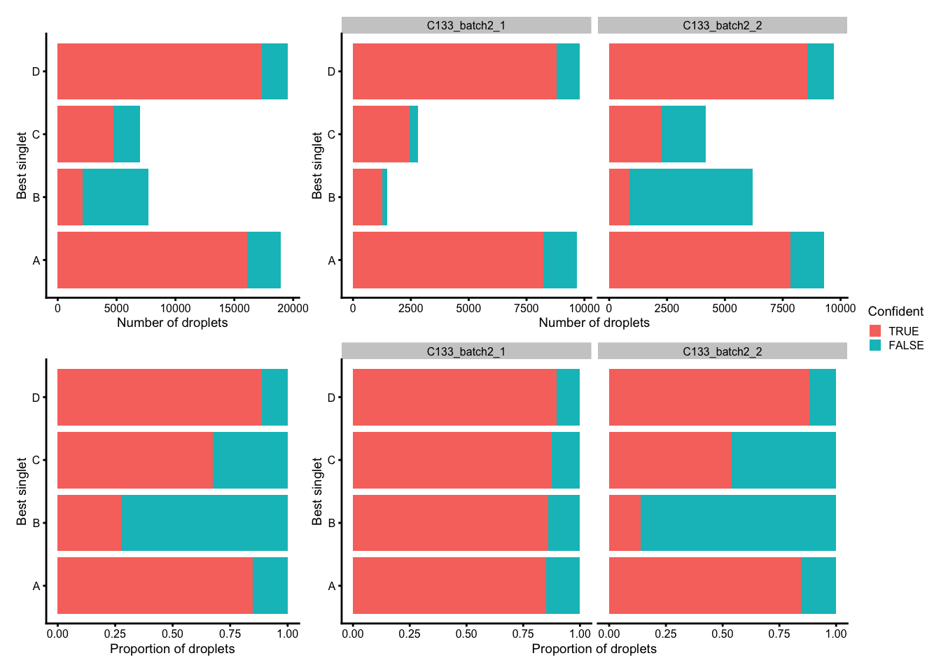
Number (top) and proportion (bottom) of droplets assigned to each donor based on genetics (best singlet), and if these were confidently or not confidently assigned, overall (left) and within each capture (right).
p3 <- ggplot(
  data.frame(
    GeneticDonor = sce$GeneticDonor,
    Confident = sce$vireo$Confident,
    Capture = sce$Capture)) +
  geom_bar(
    aes(x = GeneticDonor, fill = Confident),
    position = position_stack(reverse = TRUE)) +
  coord_flip() +
  ylab("Number of droplets") +
  xlab("Final donor assignment") +
  theme_cowplot(font_size = 7)

(p3 + p3 + facet_grid(~Capture) + plot_layout(widths = c(1, 2))) +
  plot_layout(guides = "collect")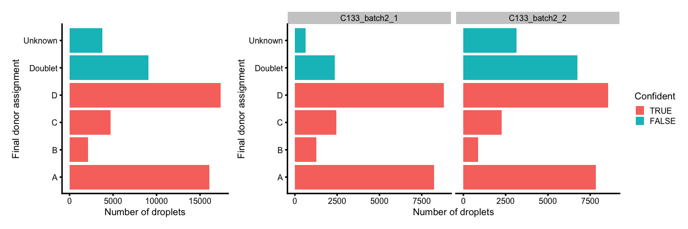
Number and proportion of droplets assigned to each donor based on genetics (final assignment), and if these were confidently or not confidently assigned, overall (left) and within each capture (right).
Overall summary
p <- scater::plotColData(
  sce,
  "dmmHTO",
  "GeneticDonor",
  colour_by = "GeneticDonor",
  other_fields = "Capture") +
  scale_x_discrete(guide = guide_axis(n.dodge = 2)) +
  guides(colour = "none")
p / (p + facet_grid(~Capture))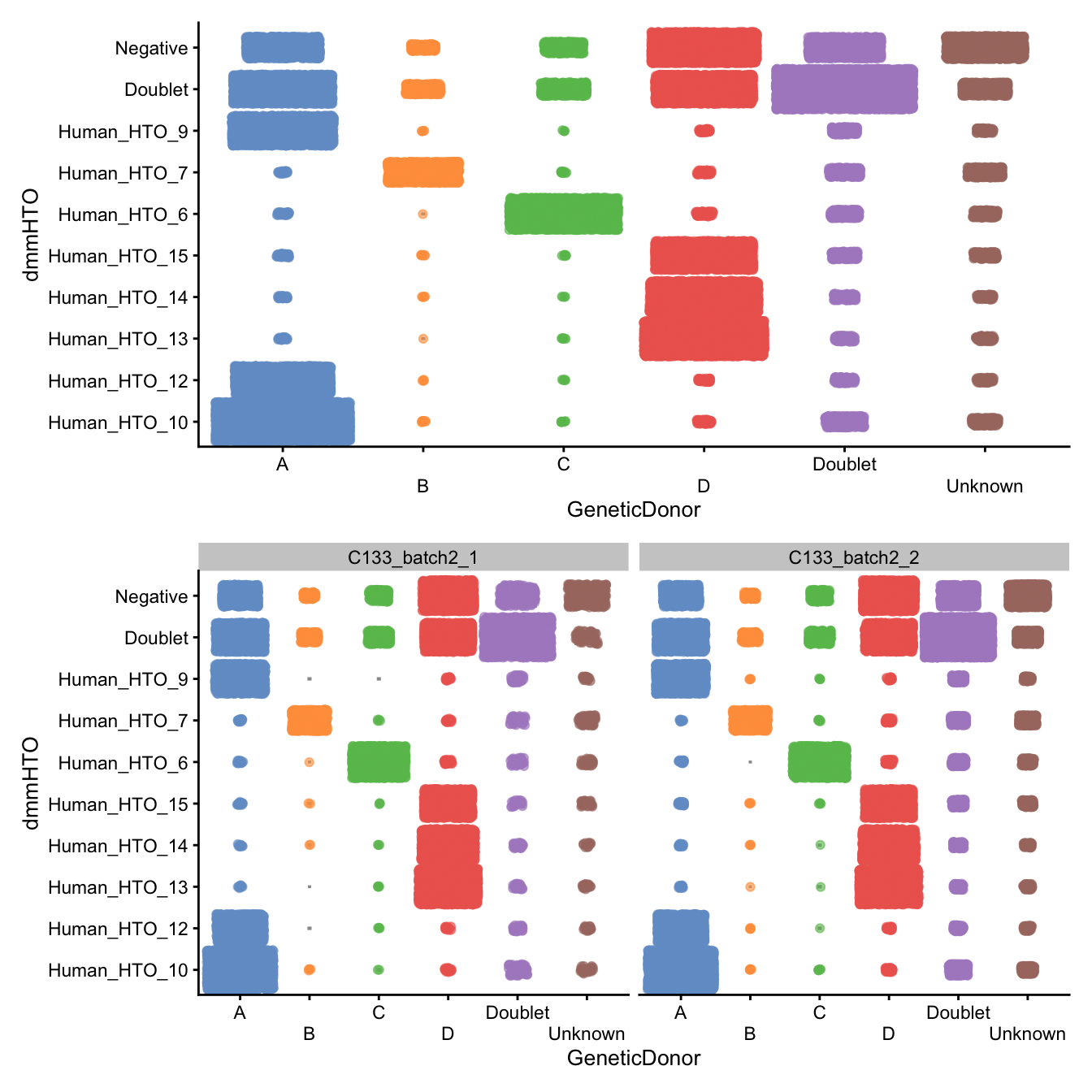
Number of droplets assigned to each
dmmHTO/GeneticDonor combination, overall (top)
and within each capture (bottom)
janitor::tabyl(
  as.data.frame(colData(sce)[, c("dmmHTO", "GeneticDonor")]),
  dmmHTO,
  GeneticDonor) |>
  janitor::adorn_title(placement = "combined") |>
  janitor::adorn_totals("both") |>
  knitr::kable(
caption = "Number of droplets assigned to each `dmmHTO`/`GeneticDonor` combination.")| dmmHTO/GeneticDonor | A | B | C | D | Doublet | Unknown | Total |
|---|---|---|---|---|---|---|---|
| Human_HTO_10 | 5424 | 9 | 8 | 67 | 463 | 215 | 6186 |
| Human_HTO_12 | 2766 | 4 | 5 | 47 | 130 | 91 | 3043 |
| Human_HTO_13 | 28 | 1 | 6 | 4350 | 125 | 103 | 4613 |
| Human_HTO_14 | 31 | 5 | 4 | 3557 | 148 | 85 | 3830 |
| Human_HTO_15 | 47 | 6 | 7 | 2901 | 210 | 170 | 3341 |
| Human_HTO_6 | 48 | 1 | 3556 | 90 | 253 | 194 | 4142 |
| Human_HTO_7 | 29 | 1544 | 11 | 66 | 303 | 374 | 2327 |
| Human_HTO_9 | 3105 | 4 | 4 | 39 | 196 | 86 | 3434 |
| Doublet | 2952 | 373 | 632 | 2896 | 5656 | 626 | 13135 |
| Negative | 1648 | 180 | 478 | 3350 | 1607 | 1846 | 9109 |
| Total | 16078 | 2127 | 4711 | 17363 | 9091 | 3790 | 53160 |
Save data
saveRDS(
   sce,
   here("data",
        "C133_Neeland_batch2",
        "data",
        "SCEs",
        "C133_Neeland_batch2.preprocessed.SCE.rds"))
Session info
sessionInfo()R version 4.3.2 (2023-10-31)
Platform: aarch64-apple-darwin20 (64-bit)
Running under: macOS Sonoma 14.3
Matrix products: default
BLAS: /Library/Frameworks/R.framework/Versions/4.3-arm64/Resources/lib/libRblas.0.dylib
LAPACK: /Library/Frameworks/R.framework/Versions/4.3-arm64/Resources/lib/libRlapack.dylib; LAPACK version 3.11.0
locale:
[1] en_US.UTF-8/en_US.UTF-8/en_US.UTF-8/C/en_US.UTF-8/en_US.UTF-8
time zone: Australia/Melbourne
tzcode source: internal
attached base packages:
[1] stats4 stats graphics grDevices datasets utils methods
[8] base
other attached packages:
[1] vcfR_1.15.0 scater_1.30.1
[3] scuttle_1.12.0 DropletUtils_1.22.0
[5] SingleCellExperiment_1.24.0 SummarizedExperiment_1.32.0
[7] Biobase_2.62.0 GenomicRanges_1.54.1
[9] GenomeInfoDb_1.38.6 IRanges_2.36.0
[11] S4Vectors_0.40.2 BiocGenerics_0.48.1
[13] MatrixGenerics_1.14.0 matrixStats_1.2.0
[15] lubridate_1.9.3 forcats_1.0.0
[17] stringr_1.5.1 dplyr_1.1.4
[19] purrr_1.0.2 readr_2.1.5
[21] tidyr_1.3.1 tibble_3.2.1
[23] tidyverse_2.0.0 demuxmix_1.4.0
[25] patchwork_1.2.0 cowplot_1.1.3
[27] ggplot2_3.4.4 BiocStyle_2.30.0
[29] readxl_1.4.3 here_1.0.1
[31] workflowr_1.7.1
loaded via a namespace (and not attached):
[1] RColorBrewer_1.1-3 rstudioapi_0.15.0
[3] jsonlite_1.8.8 magrittr_2.0.3
[5] ggbeeswarm_0.7.2 farver_2.1.1
[7] rmarkdown_2.25 fs_1.6.3
[9] zlibbioc_1.48.0 vctrs_0.6.5
[11] DelayedMatrixStats_1.24.0 RCurl_1.98-1.14
[13] janitor_2.2.0 htmltools_0.5.7
[15] S4Arrays_1.2.0 BiocNeighbors_1.20.2
[17] cellranger_1.1.0 Rhdf5lib_1.24.2
[19] SparseArray_1.2.4 rhdf5_2.46.1
[21] sass_0.4.8 bslib_0.6.1
[23] cachem_1.0.8 whisker_0.4.1
[25] lifecycle_1.0.4 pkgconfig_2.0.3
[27] rsvd_1.0.5 Matrix_1.6-5
[29] R6_2.5.1 fastmap_1.1.1
[31] snakecase_0.11.1 GenomeInfoDbData_1.2.11
[33] digest_0.6.34 colorspace_2.1-0
[35] ps_1.7.6 rprojroot_2.0.4
[37] dqrng_0.3.2 irlba_2.3.5.1
[39] vegan_2.6-4 beachmat_2.18.1
[41] labeling_0.4.3 fansi_1.0.6
[43] timechange_0.3.0 mgcv_1.9-1
[45] httr_1.4.7 abind_1.4-5
[47] compiler_4.3.2 withr_3.0.0
[49] BiocParallel_1.36.0 viridis_0.6.5
[51] highr_0.10 HDF5Array_1.30.0
[53] R.utils_2.12.3 MASS_7.3-60.0.1
[55] DelayedArray_0.28.0 permute_0.9-7
[57] tools_4.3.2 vipor_0.4.7
[59] ape_5.7-1 beeswarm_0.4.0
[61] httpuv_1.6.14 R.oo_1.26.0
[63] glue_1.7.0 callr_3.7.3
[65] nlme_3.1-164 rhdf5filters_1.14.1
[67] promises_1.2.1 grid_4.3.2
[69] getPass_0.2-4 cluster_2.1.6
[71] memuse_4.2-3 generics_0.1.3
[73] isoband_0.2.7 gtable_0.3.4
[75] tzdb_0.4.0 R.methodsS3_1.8.2
[77] pinfsc50_1.3.0 hms_1.1.3
[79] BiocSingular_1.18.0 ScaledMatrix_1.10.0
[81] utf8_1.2.4 XVector_0.42.0
[83] ggrepel_0.9.5 pillar_1.9.0
[85] limma_3.58.1 later_1.3.2
[87] splines_4.3.2 lattice_0.22-5
[89] renv_1.0.3 tidyselect_1.2.0
[91] locfit_1.5-9.8 knitr_1.45
[93] git2r_0.33.0 gridExtra_2.3
[95] edgeR_4.0.15 xfun_0.42
[97] statmod_1.5.0 pheatmap_1.0.12
[99] stringi_1.8.3 yaml_2.3.8
[101] evaluate_0.23 codetools_0.2-19
[103] BiocManager_1.30.22 cli_3.6.2
[105] munsell_0.5.0 processx_3.8.3
[107] jquerylib_0.1.4 Rcpp_1.0.12
[109] parallel_4.3.2 sparseMatrixStats_1.14.0
[111] bitops_1.0-7 viridisLite_0.4.2
[113] scales_1.3.0 crayon_1.5.2
[115] rlang_1.1.3