Demultiplexing the C133_Neeland_batch3 data set
Peter Hickey and Jovana Maksimovic
2024-02-26
Last updated: 2024-02-26
Checks: 7 0
Knit directory: paed-inflammation-CITEseq/
This reproducible R Markdown analysis was created with workflowr (version 1.7.1). The Checks tab describes the reproducibility checks that were applied when the results were created. The Past versions tab lists the development history.
Great! Since the R Markdown file has been committed to the Git repository, you know the exact version of the code that produced these results.
Great job! The global environment was empty. Objects defined in the global environment can affect the analysis in your R Markdown file in unknown ways. For reproduciblity it’s best to always run the code in an empty environment.
The command set.seed(20240216) was run prior to running
the code in the R Markdown file. Setting a seed ensures that any results
that rely on randomness, e.g. subsampling or permutations, are
reproducible.
Great job! Recording the operating system, R version, and package versions is critical for reproducibility.
Nice! There were no cached chunks for this analysis, so you can be confident that you successfully produced the results during this run.
Great job! Using relative paths to the files within your workflowr project makes it easier to run your code on other machines.
Great! You are using Git for version control. Tracking code development and connecting the code version to the results is critical for reproducibility.
The results in this page were generated with repository version 025ceae. See the Past versions tab to see a history of the changes made to the R Markdown and HTML files.
Note that you need to be careful to ensure that all relevant files for
the analysis have been committed to Git prior to generating the results
(you can use wflow_publish or
wflow_git_commit). workflowr only checks the R Markdown
file, but you know if there are other scripts or data files that it
depends on. Below is the status of the Git repository when the results
were generated:
Ignored files:
    Ignored:    .Rhistory
    Ignored:    .Rproj.user/

Untracked files:
    Untracked:  .DS_Store
    Untracked:  analysis/02.0_quality_control.Rmd
    Untracked:  analysis/03.0_call_doublets.Rmd
    Untracked:  code/dropletutils.R
    Untracked:  code/utility.R
    Untracked:  data/.DS_Store
    Untracked:  data/C133_Neeland_batch0/
    Untracked:  data/C133_Neeland_batch1/
    Untracked:  data/C133_Neeland_batch2/
    Untracked:  data/C133_Neeland_batch3/
    Untracked:  data/C133_Neeland_batch4/
    Untracked:  data/C133_Neeland_batch5/
    Untracked:  data/C133_Neeland_batch6/
    Untracked:  renv.lock
    Untracked:  renv/

Unstaged changes:
    Modified:   .Rprofile
    Modified:   .gitignore
Note that any generated files, e.g. HTML, png, CSS, etc., are not included in this status report because it is ok for generated content to have uncommitted changes.
These are the previous versions of the repository in which changes were
made to the R Markdown
(analysis/01.3_preprocess_batch3.Rmd) and HTML
(docs/01.3_preprocess_batch3.html) files. If you’ve
configured a remote Git repository (see ?wflow_git_remote),
click on the hyperlinks in the table below to view the files as they
were in that past version.
| File | Version | Author | Date | Message |
|---|---|---|---|---|
| Rmd | 025ceae | Jovana Maksimovic | 2024-02-26 | wflow_publish(c("analysis/index.Rmd", "analysis/01*")) |
suppressPackageStartupMessages({
    library(here)
    library(readxl)
    library(BiocStyle)
    library(ggplot2)
    library(cowplot)
    library(patchwork)
    library(demuxmix)
    library(tidyverse)
    library(SingleCellExperiment)
    library(DropletUtils)
    library(scater)
})
Overview
- There are 8 samples in this batch.
- Each sample comes from a different donor (i.e. each sample is genetically distinct).
- Each has a unique HTO label.
We used simple HTO labelling whereby each sample is labelled with 1 HTO, shown in the table below:
sample_metadata_df <- read_excel(
  here("data/C133_Neeland_batch3/data/sample_sheets/CITEseq_48 samples_design_2.xlsx"),
  col_types =
    c("text", "text", "text", "numeric", "text", "numeric", "text", "date"))
sample_metadata_df$`HASHTAG ID` <- paste0(
  "Human_HTO_",
  sample_metadata_df$`HASHTAG ID`)
knitr::kable(sample_metadata_df[sample_metadata_df$Batch == 3, ])| Donor | Sample name | Disease | Age | Sex | Batch | HASHTAG ID | DATE OF CAPTURE |
|---|---|---|---|---|---|---|---|
| 13 | 13 | True control | 0.8356164 | M | 3 | Human_HTO_6 | 2021-09-07 |
| 14 | 14 | True control | 1.1100000 | M | 3 | Human_HTO_7 | 2021-09-07 |
| 15 | 15 | CF | 2.9780822 | F | 3 | Human_HTO_9 | 2021-09-07 |
| 16 | 16 | CF | 3.0301370 | M | 3 | Human_HTO_10 | 2021-09-07 |
| 17 | 17 | CF | 0.9369863 | M | 3 | Human_HTO_12 | 2021-09-07 |
| 18 | 18 | CF | 0.9232877 | F | 3 | Human_HTO_13 | 2021-09-07 |
| 19 | 19 | True control | 5.3534247 | M | 3 | Human_HTO_14 | 2021-09-07 |
| 20 | 20 | True control | 4.7100000 | F | 3 | Human_HTO_15 | 2021-09-07 |
Setting up the data
sce <- readRDS(here("data", "C133_Neeland_batch3",
                    "data", "SCEs", "C133_Neeland_batch3.CellRanger.SCE.rds"))
sce$Capture <- factor(sce$Sample)
capture_names <- levels(sce$Capture)
capture_names <- setNames(capture_names, capture_names)
sce$Sample <- NULL
sce
class: SingleCellExperiment
dim: 36601 6515066
metadata(1): Samples
assays(1): counts
rownames(36601): ENSG00000243485 ENSG00000237613 ... ENSG00000278817
ENSG00000277196
rowData names(3): ID Symbol Type
colnames(6515066): 1_AAACCCAAGAAACACT-1 1_AAACCCAAGAAACCCA-1 ...
2_TTTGTTGTCTTTGCTA-1 2_TTTGTTGTCTTTGGAG-1
colData names(2): Barcode Capture
reducedDimNames(0):
mainExpName: Gene Expression
altExpNames(1): Antibody CaptureCalling cells from empty droplets
par(mfrow = c(1, 2))
lapply(capture_names, function(cn) {
  sce <- sce[, sce$Capture == cn]
  bcrank <- barcodeRanks(counts(sce))
  # Only showing unique points for plotting speed.
  uniq <- !duplicated(bcrank$rank)
  plot(
    x = bcrank$rank[uniq],
    y = bcrank$total[uniq],
    log = "xy",
    xlab = "Rank",
    ylab = "Total UMI count",
    main = cn,
    cex.lab = 1.2,
    xlim = c(1, 500000),
    ylim = c(1, 200000))
  abline(h = metadata(bcrank)$inflection, col = "darkgreen", lty = 2)
  abline(h = metadata(bcrank)$knee, col = "dodgerblue", lty = 2)
})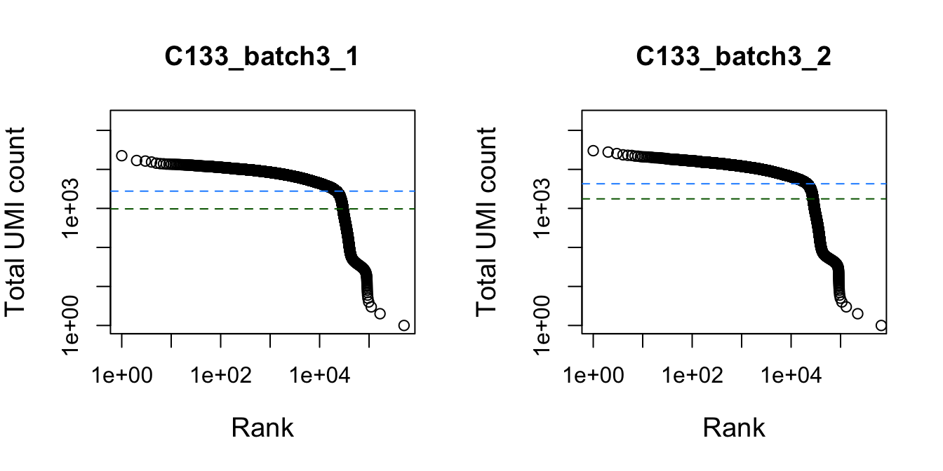
Total UMI count for each barcode in the dataset, plotted against its rank (in decreasing order of total counts). The inferred locations of the inflection (dark green dashed lines) and knee points (blue dashed lines) are also shown.
Remove empty droplets.
empties <- do.call(rbind, lapply(capture_names, function(cn) {
  message(cn)
  empties <- readRDS(
    here("data",
         "C133_Neeland_batch3",
         "data",
         "emptyDrops", paste0(cn, ".emptyDrops.rds")))
  empties$Capture <- cn
  empties
}))
tapply(
  empties$FDR,
  empties$Capture,
  function(x) sum(x <= 0.001, na.rm = TRUE)) |>
  knitr::kable(
caption = "Number of non-empty droplets identified using `emptyDrops()` from **DropletUtils**.")| x | |
|---|---|
| C133_batch3_1 | 32886 |
| C133_batch3_2 | 31956 |
sce <- sce[, which(empties$FDR <= 0.001)]
sce
class: SingleCellExperiment
dim: 36601 64842
metadata(1): Samples
assays(1): counts
rownames(36601): ENSG00000243485 ENSG00000237613 ... ENSG00000278817
ENSG00000277196
rowData names(3): ID Symbol Type
colnames(64842): 1_AAACCCAAGCAGCACA-1 1_AAACCCAAGCATCTTG-1 ...
2_TTTGTTGTCTAGGCCG-1 2_TTTGTTGTCTCGGCTT-1
colData names(2): Barcode Capture
reducedDimNames(0):
mainExpName: Gene Expression
altExpNames(1): Antibody CaptureAdding per cell quality control information
sce <- scuttle::addPerCellQC(sce)
head(colData(sce)) %>%
  data.frame %>%
knitr::kable()| Barcode | Capture | sum | detected | altexps_Antibody.Capture_sum | altexps_Antibody.Capture_detected | altexps_Antibody.Capture_percent | total | |
|---|---|---|---|---|---|---|---|---|
| 1_AAACCCAAGCAGCACA-1 | AAACCCAAGCAGCACA-1 | C133_batch3_1 | 5231 | 1787 | 3818 | 164 | 42.19251 | 9049 |
| 1_AAACCCAAGCATCTTG-1 | AAACCCAAGCATCTTG-1 | C133_batch3_1 | 3112 | 1302 | 2583 | 158 | 45.35558 | 5695 |
| 1_AAACCCAAGGTAGATT-1 | AAACCCAAGGTAGATT-1 | C133_batch3_1 | 2117 | 1147 | 1411 | 155 | 39.99433 | 3528 |
| 1_AAACCCAAGGTGGTTG-1 | AAACCCAAGGTGGTTG-1 | C133_batch3_1 | 5032 | 1987 | 3546 | 165 | 41.33831 | 8578 |
| 1_AAACCCAAGGTGTGAC-1 | AAACCCAAGGTGTGAC-1 | C133_batch3_1 | 3659 | 1415 | 3276 | 161 | 47.23864 | 6935 |
| 1_AAACCCAAGTAAAGCT-1 | AAACCCAAGTAAAGCT-1 | C133_batch3_1 | 5344 | 2142 | 2844 | 164 | 34.73376 | 8188 |
Demultiplexing with hashtag oligos (HTOs)
is_adt <- grepl("^A[0-9]+", rownames(altExp(sce, "Antibody Capture")))
is_hto <- grepl("^Human_HTO", rownames(altExp(sce, "Antibody Capture")))
altExp(sce, "HTO") <- altExp(sce, "Antibody Capture")[is_hto, ]
altExp(sce, "ADT") <- altExp(sce, "Antibody Capture")[is_adt, ]
altExp(sce, "Antibody Capture") <- NULL
hto_counts <- counts(altExp(sce, "HTO"))
xmax <- ceiling(max(log2(hto_counts + 1)))
C133_batch3_1
par(mfrow = c(3, 3))
lapply(rownames(hto_counts), function(i) {
  hist(
    log2(hto_counts[i, sce$Capture == "C133_batch3_1"] + 1),
    xlab = "log2(UMIs + 1)",
    main = paste0("C133_1: ", i),
    xlim = c(0, xmax),
    breaks = seq(0, xmax, 0.5),
    cex.main = 0.8)
})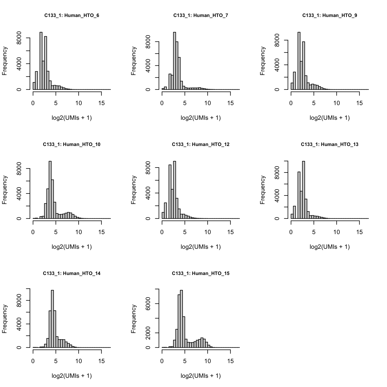
Number of UMIs for each HTO across all non-empty droplets.
Prepare the data.
hto <- as.matrix(counts(altExp(sce[, sce$Capture == "C133_batch3_1"], "HTO")))
detected <- sce$detected[sce$Capture == "C133_batch3_1"]

df <- data.frame(t(hto),
                 detected = detected,
                 hto = colSums(hto))

df %>%
  pivot_longer(cols = starts_with("Human_HTO")) %>%
  mutate(logged = log(value + 1)) %>%
  ggplot(aes(x = logged)) +
  geom_density(adjust = 5) +
  facet_wrap(~name, scales = "free")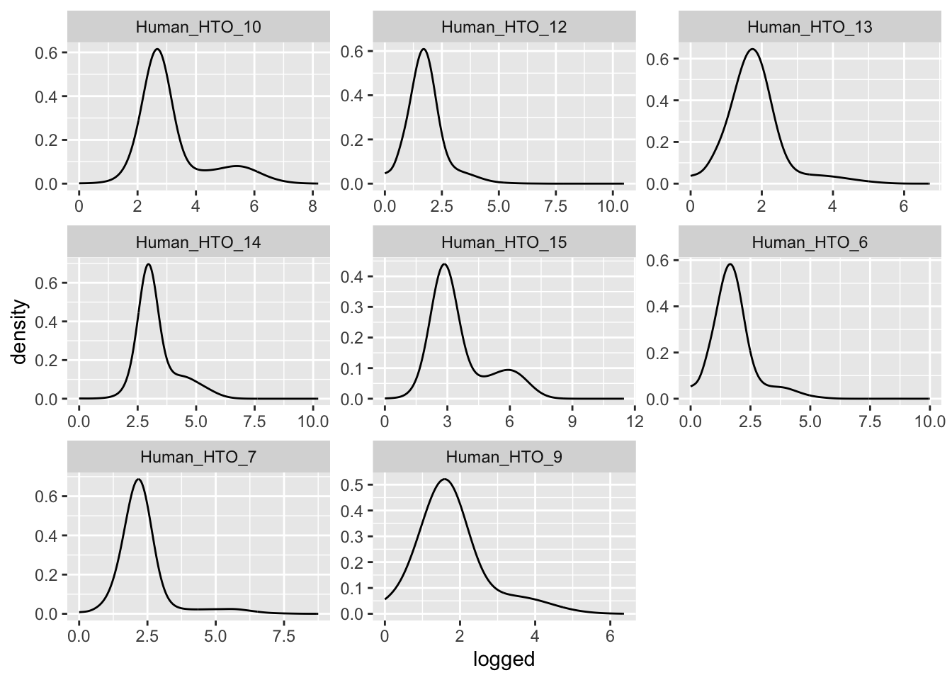
df %>%
  pivot_longer(cols = starts_with("Human_HTO")) %>%
  ggplot(aes(x = detected, y = hto)) +
  geom_density_2d() +
facet_wrap(~name) 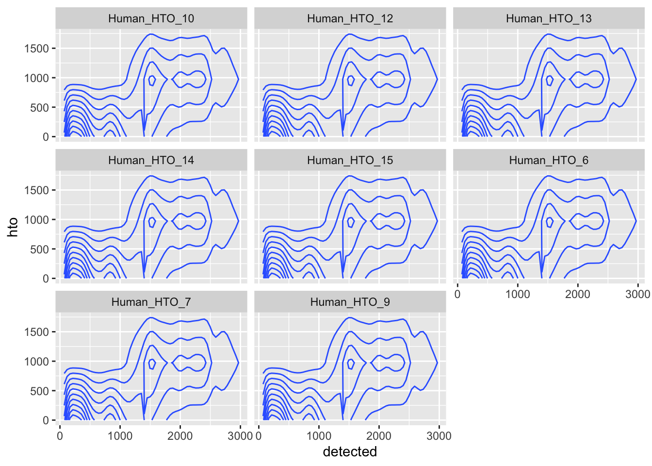
Run demultiplexing.
dmm <- demuxmix(hto = hto,
                rna = detected,
                model = "naive")
summary(dmm)
Class NumObs RelFreq MedProb ExpFPs FDR
1 Human_HTO_10 3174 0.10097989 0.8136211 704.4033 0.2219292
2 Human_HTO_12 1235 0.03929117 0.8170094 287.8670 0.2330907
3 Human_HTO_13 1152 0.03665055 0.8088967 264.3463 0.2294673
4 Human_HTO_14 3899 0.12404556 0.8619341 726.0888 0.1862244
5 Human_HTO_15 4485 0.14268898 0.8150755 993.9092 0.2216074
6 Human_HTO_6 1243 0.03954569 0.8169106 275.3550 0.2215245
7 Human_HTO_7 1141 0.03630059 0.8214862 247.2973 0.2167373
8 Human_HTO_9 2212 0.07037414 0.8182160 496.5877 0.2244971
9 singlet 18541 0.58987656 0.8233318 3995.8546 0.2155145
10 multiplet 7671 0.24405065 0.7782242 2007.0453 0.2616406
11 negative 5220 0.16607279 0.7744566 1372.8035 0.2629892
12 uncertain 1454 NA NA NA NAExamine results.
p <- vector("list", nrow(hto))
for(i in 1:nrow(hto)){
  p[[i]] <- plotDmmHistogram(dmm, hto = i) +
    coord_cartesian(ylim = c(0, 0.001),
                    xlim = c(-50, 1000)) +
    theme(axis.title = element_text(size = 8),
          axis.text = element_text(size = 6))
}

wrap_plots(p , ncol = 3) 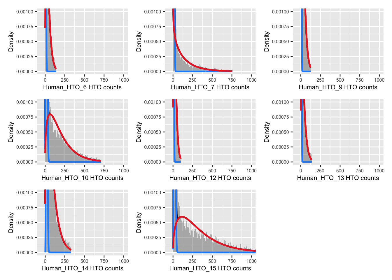
p <- vector("list", nrow(hto))
for(i in 1:nrow(hto)){
  p[[i]] <- plotDmmPosteriorP(dmm, hto = i) +
    theme(axis.title = element_text(size = 8),
          axis.text = element_text(size = 6))
}

wrap_plots(p , ncol = 3) 
pAcpt(dmm) <- 0
classes1 <- dmmClassify(dmm)
classes1$dmmHTO <- ifelse(classes1$Type == "multiplet", "Doublet",
                           ifelse(classes1$Type %in% c("negative", "uncertain"),
                                  "Negative", classes1$HTO))
table(classes1$dmmHTO)
     Doublet Human_HTO_10 Human_HTO_12 Human_HTO_13 Human_HTO_14 Human_HTO_15
        8524         3239         1271         1177         3967         4566
 Human_HTO_6  Human_HTO_7  Human_HTO_9     Negative
        1264         1163         2275         5440
C133_batch3_2
par(mfrow = c(3, 3))
lapply(rownames(hto_counts), function(i) {
  hist(
    log2(hto_counts[i, sce$Capture == "C133_batch3_2"] + 1),
    xlab = "log2(UMIs + 1)",
    main = paste0("C133_2: ", i),
    xlim = c(0, xmax),
    breaks = seq(0, xmax, 0.5),
    cex.main = 0.8)
})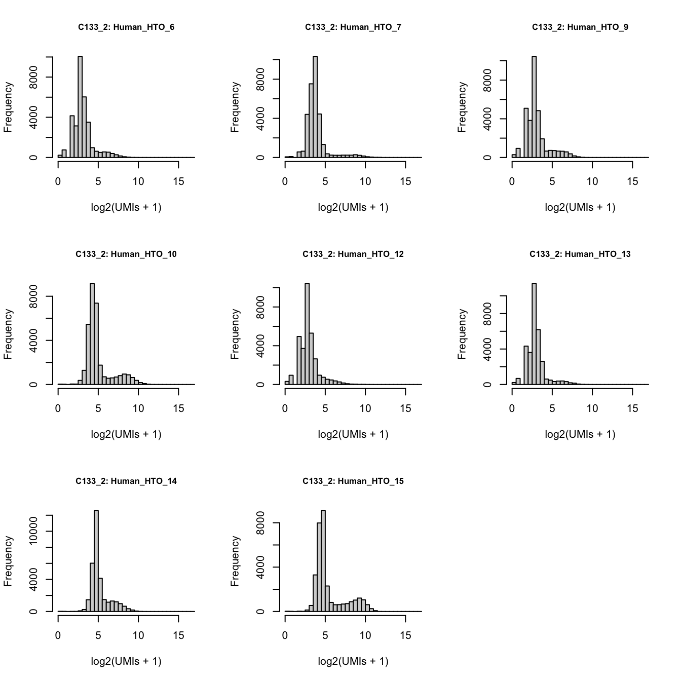
Number of UMIs for each HTO across all non-empty droplets.
Prepare the data.
hto <- as.matrix(counts(altExp(sce[, sce$Capture == "C133_batch3_2"], "HTO")))
detected <- sce$detected[sce$Capture == "C133_batch3_2"]

df <- data.frame(t(hto),
                 detected = detected,
                 hto = colSums(hto))

df %>%
  pivot_longer(cols = starts_with("Human_HTO")) %>%
  mutate(logged = log(value + 1)) %>%
  ggplot(aes(x = logged)) +
  geom_density(adjust = 5) +
  facet_wrap(~name, scales = "free")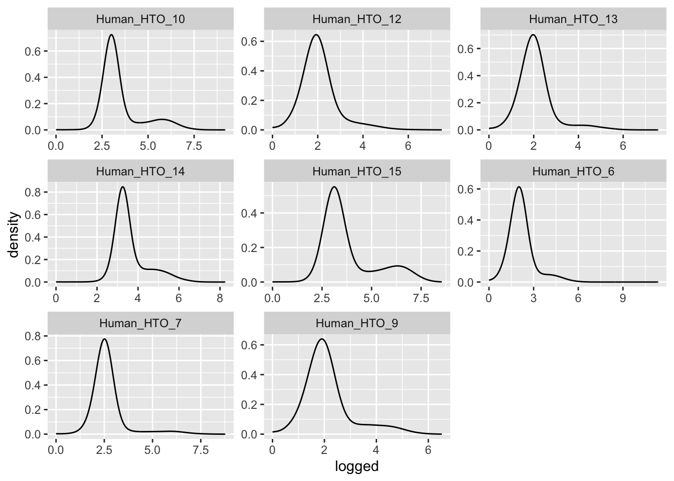
df %>%
  pivot_longer(cols = starts_with("Human_HTO")) %>%
  ggplot(aes(x = detected, y = hto)) +
  geom_density_2d() +
facet_wrap(~name) 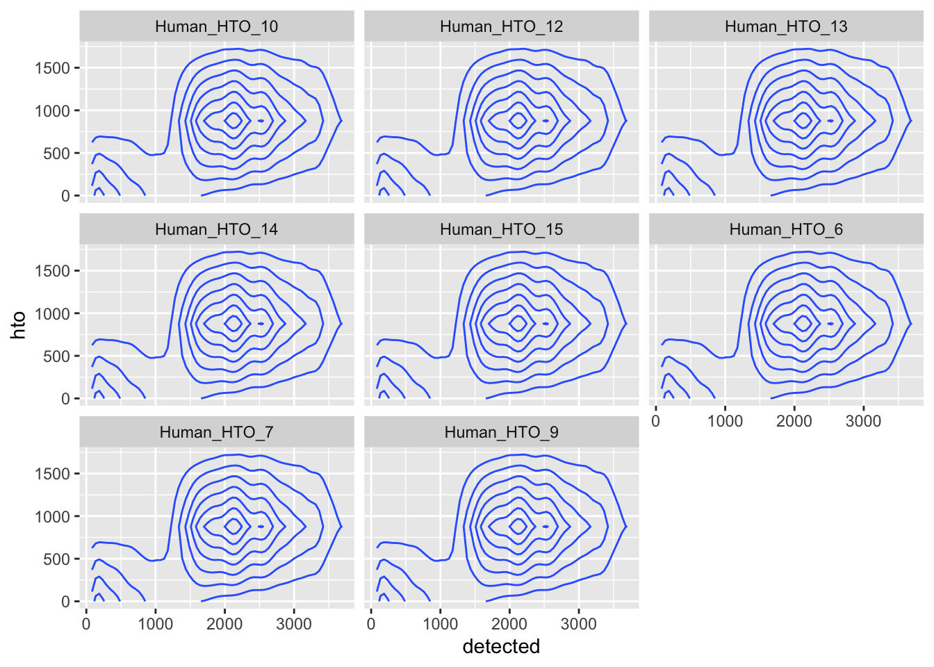
Run demultiplexing.
dmm <- demuxmix(hto = hto,
                rna = detected,
                model = "naive")
summary(dmm)
Class NumObs RelFreq MedProb ExpFPs FDR
1 Human_HTO_10 3222 0.10464437 0.8187529 698.8275 0.2168925
2 Human_HTO_12 1469 0.04771030 0.8445190 301.2351 0.2050613
3 Human_HTO_13 1258 0.04085742 0.8162974 281.9072 0.2240916
4 Human_HTO_14 3960 0.12861319 0.8518039 756.8450 0.1911225
5 Human_HTO_15 4509 0.14644365 0.8202735 960.6401 0.2130495
6 Human_HTO_6 1257 0.04082494 0.8222346 270.3173 0.2150496
7 Human_HTO_7 1138 0.03696005 0.8231691 246.5363 0.2166400
8 Human_HTO_9 2318 0.07528418 0.8228768 503.0567 0.2170219
9 singlet 19131 0.62133810 0.8274974 4019.3652 0.2100970
10 multiplet 7677 0.24933420 0.8032838 1884.7926 0.2455116
11 negative 3982 0.12932770 0.7674019 1078.4061 0.2708202
12 uncertain 1166 NA NA NA NAExamine results.
p <- vector("list", nrow(hto))
for(i in 1:nrow(hto)){
  p[[i]] <- plotDmmHistogram(dmm, hto = i) +
    coord_cartesian(ylim = c(0, 0.001),
                    xlim = c(-50, 1000)) +
    theme(axis.title = element_text(size = 8),
          axis.text = element_text(size = 6))
}

wrap_plots(p , ncol = 3) 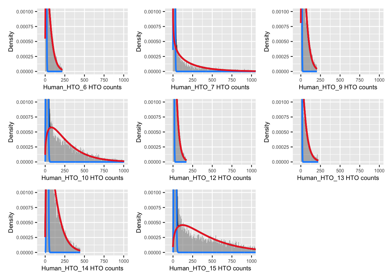
p <- vector("list", nrow(hto))
for(i in 1:nrow(hto)){
  p[[i]] <- plotDmmPosteriorP(dmm, hto = i) +
    theme(axis.title = element_text(size = 8),
          axis.text = element_text(size = 6))
}

wrap_plots(p , ncol = 3) 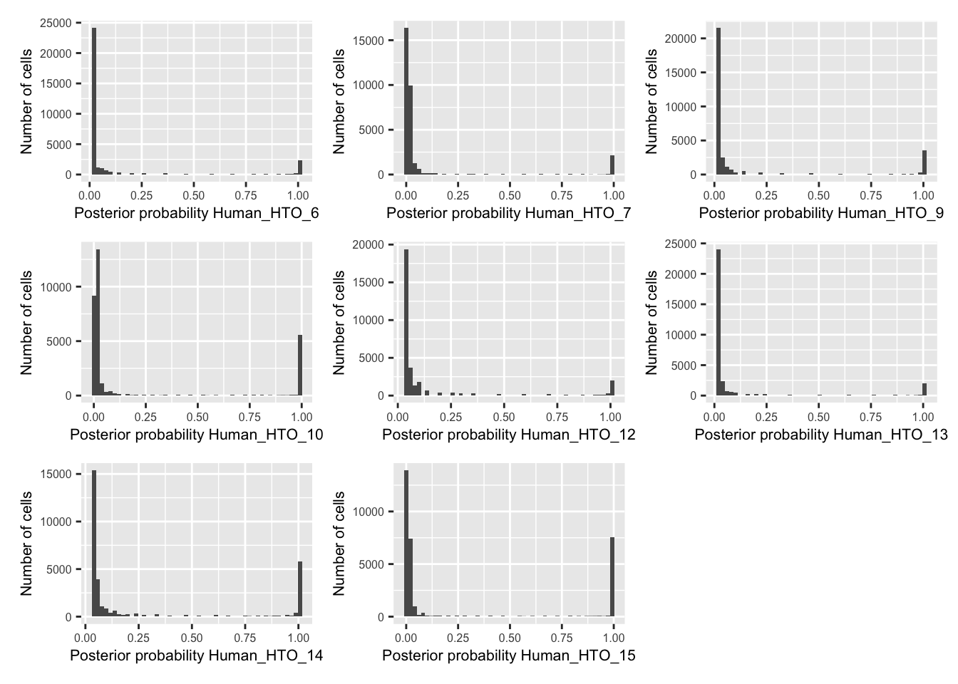
pAcpt(dmm) <- 0
classes2 <- dmmClassify(dmm)
classes2$dmmHTO <- ifelse(classes2$Type == "multiplet", "Doublet",
                           ifelse(classes2$Type %in% c("negative", "uncertain"),
                                  "Negative", classes2$HTO))
table(classes2$dmmHTO)
     Doublet Human_HTO_10 Human_HTO_12 Human_HTO_13 Human_HTO_14 Human_HTO_15
        8318         3272         1493         1292         4027         4583
 Human_HTO_6  Human_HTO_7  Human_HTO_9     Negative
        1280         1153         2362         4176
Save HTO assignments
classes <- rbind(classes1, classes2)
all(rownames(classes) == colnames(sce))
[1] TRUEsce$dmmHTO <- factor(classes$dmmHTO,
levels = c(sort(unique(grep("Human",
classes$dmmHTO,
value = TRUE))),
"Doublet",
"Negative"))Demultiplexing cells without genotype reference
Matching donors across captures
library(vcfR)
f <- sapply(capture_names, function(cn) {
  here("data",
       "C133_Neeland_batch3",
       "data",
       "vireo", cn, "GT_donors.vireo.vcf.gz")
})
x <- lapply(f, read.vcfR, verbose = FALSE)
# Create unique ID for each locus in each capture.
y <- lapply(x, function(xx) {
  paste(
  xx@fix[,"CHROM"],
  xx@fix[,"POS"],
  xx@fix[,"REF"],
  xx@fix[,"ALT"],
  sep = "_")
})
# Only keep the loci in common between the 2 captures.
i <- lapply(y, function(yy) {
  na.omit(match(Reduce(intersect, y), yy))
})
# Construct genotype matrix at common loci from the 2 captures.
donor_names <- paste0("donor", 0:7)
g <- mapply(
  function(xx, ii) {
    apply(
      xx@gt[ii, donor_names],
      2,
      function(x) sapply(strsplit(x, ":"), `[[`, 1))
  },
  xx = x,
  ii = i,
  SIMPLIFY = FALSE)
# Count number of genotype matches between pairs of donors (one from each
# capture) and convert to a proportion.
z <- lapply(2:length(capture_names), function(k) {
  zz <- matrix(
    NA_real_,
    nrow = length(donor_names),
    ncol = length(donor_names),
    dimnames = list(donor_names, donor_names))
  for (ii in rownames(zz)) {
    for (jj in colnames(zz)) {
      zz[ii, jj] <- sum(g[[1]][, ii] == g[[k]][, jj]) / nrow(g[[1]])
    }
  }
  zz
})
heatmaps <- lapply(seq_along(z), function(k) {
pheatmap::pheatmap(
z[[k]],
color = viridisLite::inferno(101),
cluster_rows = FALSE,
cluster_cols = FALSE,
main = "Proportion of matching genotypes",
display_numbers = TRUE,
number_color = "grey50",
labels_row = paste0("C133_batch3_1: ", rownames(z[[k]])),
labels_col = paste0("C133_batch3_", k + 1, ": ", colnames(z[[k]])),
silent = TRUE,
fontsize = 10)
})
gridExtra::grid.arrange(grobs = lapply(heatmaps, `[[`, "gtable"), ncol = 1)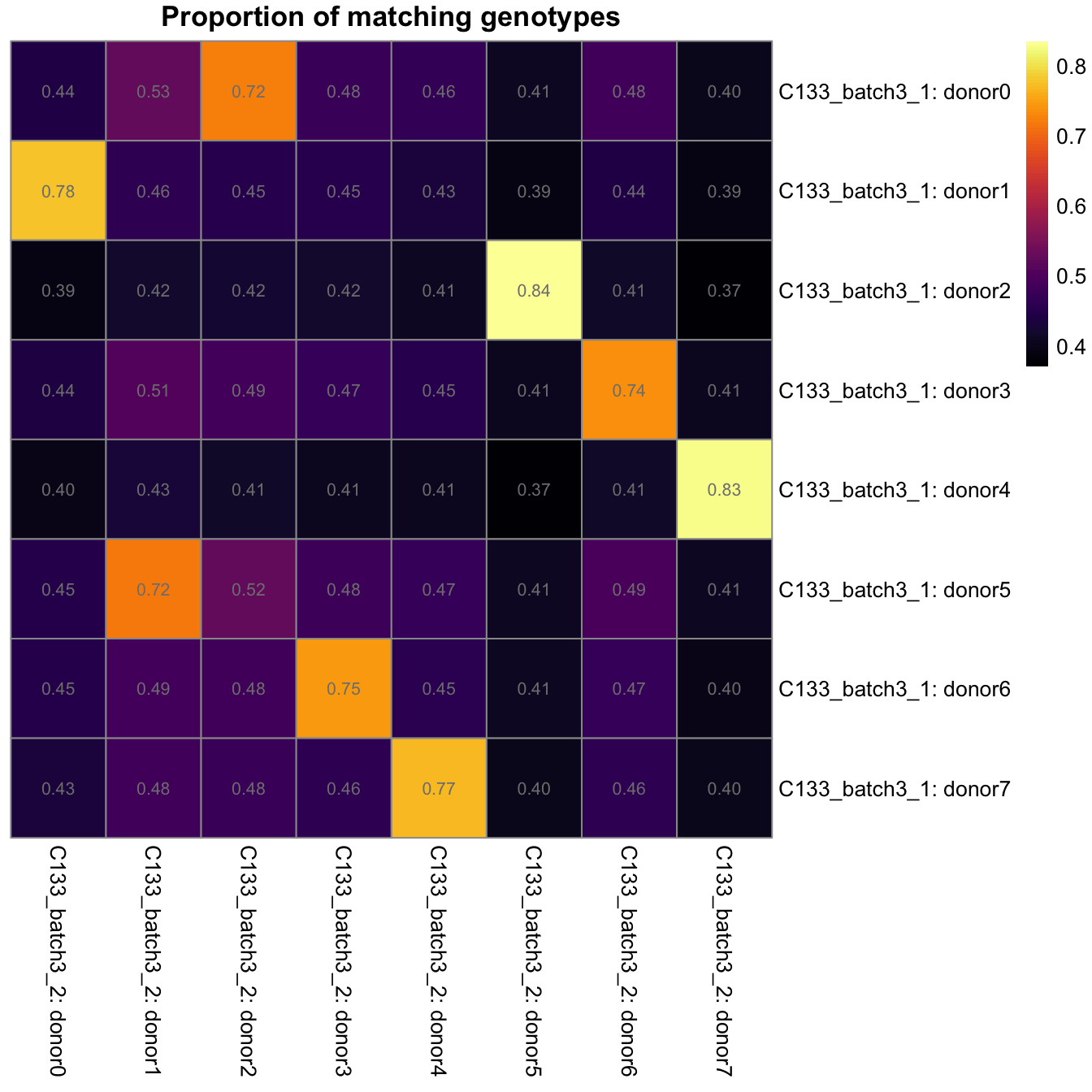
Proportion of matching genotypes between pairs of captures.
The table below gives the best matches between the captures.
best_match_df <- data.frame(
  c(
    list(rownames(z[[1]])),
    lapply(seq_along(z), function(k) {
      apply(
        z[[k]],
        1,
        function(x) colnames(z[[k]])[which.max(x)])
    })),
  row.names = NULL)
colnames(best_match_df) <- capture_names
best_match_df$GeneticDonor <- LETTERS[seq_along(donor_names)]
best_match_df <- dplyr::select(best_match_df, GeneticDonor, everything())

knitr::kable(
  best_match_df,
caption = "Best match of donors between the scRNA-seq captures.")| GeneticDonor | C133_batch3_1 | C133_batch3_2 |
|---|---|---|
| A | donor0 | donor2 |
| B | donor1 | donor0 |
| C | donor2 | donor5 |
| D | donor3 | donor6 |
| E | donor4 | donor7 |
| F | donor5 | donor1 |
| G | donor6 | donor3 |
| H | donor7 | donor4 |
Assigning barcodes to donors
vireo_df <- do.call(
  rbind,
  c(
    lapply(capture_names, function(cn) {
      # Read data
      vireo_df <- read.table(
        here("data",
             "C133_Neeland_batch3",
             "data",
             "vireo", cn, "donor_ids.tsv"),
        header = TRUE)

      # Replace `donor[0-9]+` with `donor_[A-Z]` using `best_match_df`.
      best_match <- setNames(
        c(best_match_df[["GeneticDonor"]], "Doublet", "Unknown"),
        c(best_match_df[[cn]], "doublet", "unassigned"))
      vireo_df$GeneticDonor <- factor(
        best_match[vireo_df$donor_id],
        levels = c(best_match_df[["GeneticDonor"]], "Doublet", "Unknown"))
      vireo_df$donor_id <- NULL
      vireo_df$best_singlet <- best_match[vireo_df$best_singlet]
      vireo_df$best_doublet <- sapply(
        strsplit(vireo_df$best_doublet, ","),
        function(x) {
          paste0(best_match[x[[1]]], ",", best_match[x[[2]]])
        })

      # Add additional useful metadata
      vireo_df$Confident <- factor(
        vireo_df$GeneticDonor == vireo_df$best_singlet,
        levels = c(TRUE, FALSE))
      vireo_df$Capture <- cn

      # Reorder so matches SCE.
      captureNumber <- sub("C133_batch3_", "", cn)
      vireo_df$colname <- paste0(captureNumber, "_", vireo_df$cell)
      j <- match(colnames(sce)[sce$Capture == cn], vireo_df$colname)
      stopifnot(!anyNA(j))
      vireo_df <- vireo_df[j, ]
      vireo_df
    }),
    list(make.row.names = FALSE)))
Vireo summary
We add the parsed outputs of vireo to the colData of the SingleCellExperiment object so that we can incorporate it into downstream analyses.
stopifnot(identical(colnames(sce), vireo_df$colname))
sce$GeneticDonor <- vireo_df$GeneticDonor
# NOTE: We exclude redundant columns.
sce$vireo <- DataFrame(
  vireo_df[, setdiff(
    colnames(vireo_df),
    c("cell", "colname", "Capture", "GeneticDonor"))])
tmp_df <- data.frame(
best_singlet = sce$vireo$best_singlet,
Confident = sce$vireo$Confident,
Capture = sce$Capture)
p1 <- ggplot(tmp_df) +
geom_bar(
aes(x = best_singlet, fill = Confident),
position = position_stack(reverse = TRUE)) +
coord_flip() +
ylab("Number of droplets") +
xlab("Best singlet") +
theme_cowplot(font_size = 7)
p2 <- ggplot(tmp_df) +
geom_bar(
aes(x = best_singlet, fill = Confident),
position = position_fill(reverse = TRUE)) +
coord_flip() +
ylab("Proportion of droplets") +
xlab("Best singlet") +
theme_cowplot(font_size = 7)
(p1 + p1 + facet_grid(~Capture) + plot_layout(widths = c(1, 2))) /
(p2 + p2 + facet_grid(~Capture) + plot_layout(widths = c(1, 2))) +
plot_layout(guides = "collect")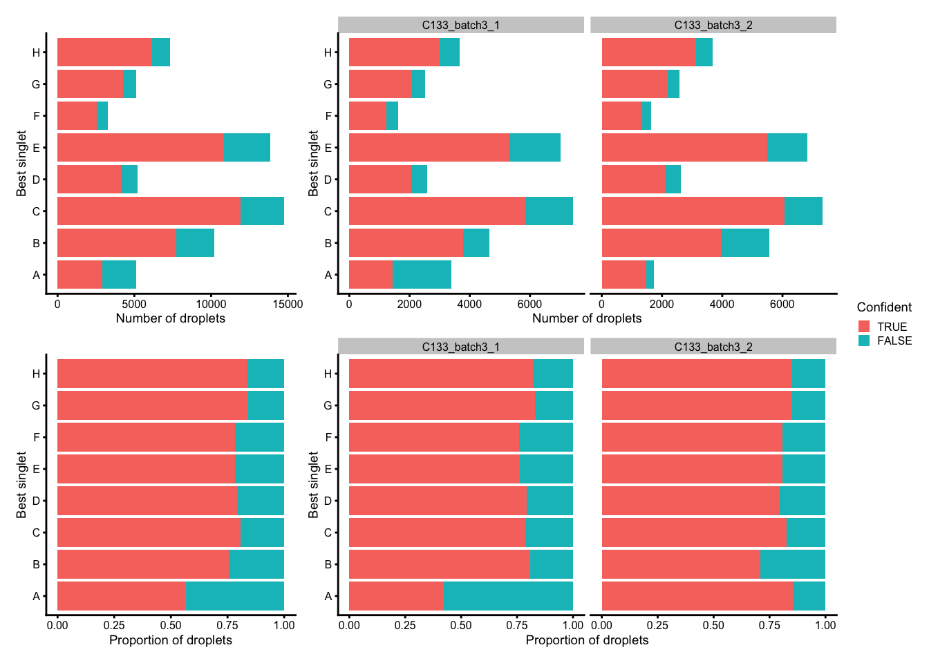
Number (top) and proportion (bottom) of droplets assigned to each donor based on genetics (best singlet), and if these were confidently or not confidently assigned, overall (left) and within each capture (right).
p3 <- ggplot(
  data.frame(
    GeneticDonor = sce$GeneticDonor,
    Confident = sce$vireo$Confident,
    Capture = sce$Capture)) +
  geom_bar(
    aes(x = GeneticDonor, fill = Confident),
    position = position_stack(reverse = TRUE)) +
  coord_flip() +
  ylab("Number of droplets") +
  xlab("Final donor assignment") +
  theme_cowplot(font_size = 7)

(p3 + p3 + facet_grid(~Capture) + plot_layout(widths = c(1, 2))) +
  plot_layout(guides = "collect")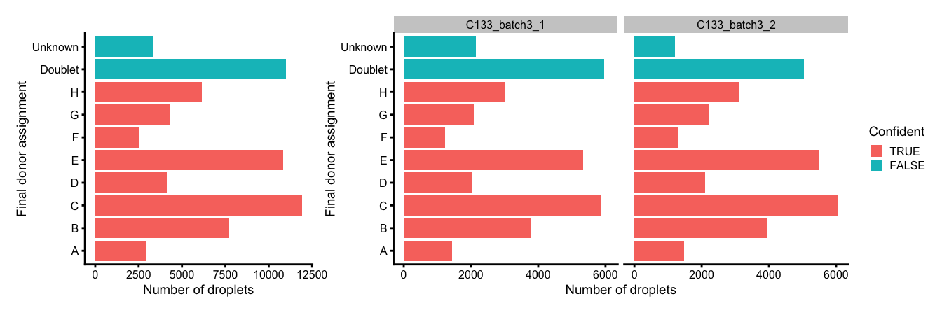
Number and proportion of droplets assigned to each donor based on genetics (final assignment), and if these were confidently or not confidently assigned, overall (left) and within each capture (right).
Overall summary
p <- scater::plotColData(
  sce,
  "dmmHTO",
  "GeneticDonor",
  colour_by = "GeneticDonor",
  other_fields = "Capture") +
  scale_x_discrete(guide = guide_axis(n.dodge = 2)) +
  guides(colour = "none")
p / (p + facet_grid(~Capture))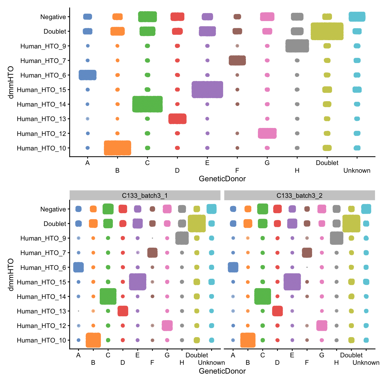
Number of droplets assigned to each
dmmHTO/GeneticDonor combination, overall (top)
and within each capture (bottom)
janitor::tabyl(
  as.data.frame(colData(sce)[, c("dmmHTO", "GeneticDonor")]),
  dmmHTO,
  GeneticDonor) |>
  janitor::adorn_title(placement = "combined") |>
  janitor::adorn_totals("both") |>
  knitr::kable(
caption = "Number of droplets assigned to each `dmmHTO`/`GeneticDonor` combination.")| dmmHTO/GeneticDonor | A | B | C | D | E | F | G | H | Doublet | Unknown | Total |
|---|---|---|---|---|---|---|---|---|---|---|---|
| Human_HTO_10 | 6 | 5923 | 39 | 26 | 13 | 4 | 27 | 17 | 328 | 128 | 6511 |
| Human_HTO_12 | 5 | 10 | 46 | 29 | 7 | 2 | 2425 | 15 | 110 | 115 | 2764 |
| Human_HTO_13 | 1 | 3 | 26 | 2262 | 5 | 0 | 14 | 12 | 92 | 54 | 2469 |
| Human_HTO_14 | 3 | 10 | 7548 | 15 | 7 | 6 | 24 | 17 | 280 | 84 | 7994 |
| Human_HTO_15 | 9 | 15 | 59 | 22 | 8201 | 5 | 36 | 22 | 428 | 352 | 9149 |
| Human_HTO_6 | 2148 | 11 | 47 | 26 | 14 | 2 | 32 | 11 | 120 | 133 | 2544 |
| Human_HTO_7 | 5 | 6 | 37 | 20 | 6 | 1948 | 20 | 19 | 112 | 143 | 2316 |
| Human_HTO_9 | 3 | 5 | 35 | 27 | 11 | 1 | 15 | 4240 | 173 | 127 | 4637 |
| Doublet | 404 | 1244 | 1630 | 577 | 1923 | 400 | 447 | 920 | 8957 | 340 | 16842 |
| Negative | 315 | 494 | 2452 | 1140 | 655 | 184 | 1245 | 861 | 404 | 1866 | 9616 |
| Total | 2899 | 7721 | 11919 | 4144 | 10842 | 2552 | 4285 | 6134 | 11004 | 3342 | 64842 |
Save data
saveRDS(
   sce,
   here("data",
        "C133_Neeland_batch3",
        "data",
        "SCEs",
        "C133_Neeland_batch3.preprocessed.SCE.rds"))
Session info
sessionInfo()R version 4.3.2 (2023-10-31)
Platform: aarch64-apple-darwin20 (64-bit)
Running under: macOS Sonoma 14.3
Matrix products: default
BLAS: /Library/Frameworks/R.framework/Versions/4.3-arm64/Resources/lib/libRblas.0.dylib
LAPACK: /Library/Frameworks/R.framework/Versions/4.3-arm64/Resources/lib/libRlapack.dylib; LAPACK version 3.11.0
locale:
[1] en_US.UTF-8/en_US.UTF-8/en_US.UTF-8/C/en_US.UTF-8/en_US.UTF-8
time zone: Australia/Melbourne
tzcode source: internal
attached base packages:
[1] stats4 stats graphics grDevices datasets utils methods
[8] base
other attached packages:
[1] vcfR_1.15.0 scater_1.30.1
[3] scuttle_1.12.0 DropletUtils_1.22.0
[5] SingleCellExperiment_1.24.0 SummarizedExperiment_1.32.0
[7] Biobase_2.62.0 GenomicRanges_1.54.1
[9] GenomeInfoDb_1.38.6 IRanges_2.36.0
[11] S4Vectors_0.40.2 BiocGenerics_0.48.1
[13] MatrixGenerics_1.14.0 matrixStats_1.2.0
[15] lubridate_1.9.3 forcats_1.0.0
[17] stringr_1.5.1 dplyr_1.1.4
[19] purrr_1.0.2 readr_2.1.5
[21] tidyr_1.3.1 tibble_3.2.1
[23] tidyverse_2.0.0 demuxmix_1.4.0
[25] patchwork_1.2.0 cowplot_1.1.3
[27] ggplot2_3.4.4 BiocStyle_2.30.0
[29] readxl_1.4.3 here_1.0.1
[31] workflowr_1.7.1
loaded via a namespace (and not attached):
[1] RColorBrewer_1.1-3 rstudioapi_0.15.0
[3] jsonlite_1.8.8 magrittr_2.0.3
[5] ggbeeswarm_0.7.2 farver_2.1.1
[7] rmarkdown_2.25 fs_1.6.3
[9] zlibbioc_1.48.0 vctrs_0.6.5
[11] DelayedMatrixStats_1.24.0 RCurl_1.98-1.14
[13] janitor_2.2.0 htmltools_0.5.7
[15] S4Arrays_1.2.0 BiocNeighbors_1.20.2
[17] cellranger_1.1.0 Rhdf5lib_1.24.2
[19] SparseArray_1.2.4 rhdf5_2.46.1
[21] sass_0.4.8 bslib_0.6.1
[23] cachem_1.0.8 whisker_0.4.1
[25] lifecycle_1.0.4 pkgconfig_2.0.3
[27] rsvd_1.0.5 Matrix_1.6-5
[29] R6_2.5.1 fastmap_1.1.1
[31] snakecase_0.11.1 GenomeInfoDbData_1.2.11
[33] digest_0.6.34 colorspace_2.1-0
[35] ps_1.7.6 rprojroot_2.0.4
[37] dqrng_0.3.2 irlba_2.3.5.1
[39] vegan_2.6-4 beachmat_2.18.1
[41] labeling_0.4.3 fansi_1.0.6
[43] timechange_0.3.0 mgcv_1.9-1
[45] httr_1.4.7 abind_1.4-5
[47] compiler_4.3.2 withr_3.0.0
[49] BiocParallel_1.36.0 viridis_0.6.5
[51] highr_0.10 HDF5Array_1.30.0
[53] R.utils_2.12.3 MASS_7.3-60.0.1
[55] DelayedArray_0.28.0 permute_0.9-7
[57] tools_4.3.2 vipor_0.4.7
[59] ape_5.7-1 beeswarm_0.4.0
[61] httpuv_1.6.14 R.oo_1.26.0
[63] glue_1.7.0 callr_3.7.3
[65] nlme_3.1-164 rhdf5filters_1.14.1
[67] promises_1.2.1 grid_4.3.2
[69] getPass_0.2-4 cluster_2.1.6
[71] memuse_4.2-3 generics_0.1.3
[73] isoband_0.2.7 gtable_0.3.4
[75] tzdb_0.4.0 R.methodsS3_1.8.2
[77] pinfsc50_1.3.0 hms_1.1.3
[79] BiocSingular_1.18.0 ScaledMatrix_1.10.0
[81] utf8_1.2.4 XVector_0.42.0
[83] ggrepel_0.9.5 pillar_1.9.0
[85] limma_3.58.1 later_1.3.2
[87] splines_4.3.2 lattice_0.22-5
[89] renv_1.0.3 tidyselect_1.2.0
[91] locfit_1.5-9.8 knitr_1.45
[93] git2r_0.33.0 gridExtra_2.3
[95] edgeR_4.0.15 xfun_0.42
[97] statmod_1.5.0 pheatmap_1.0.12
[99] stringi_1.8.3 yaml_2.3.8
[101] evaluate_0.23 codetools_0.2-19
[103] BiocManager_1.30.22 cli_3.6.2
[105] munsell_0.5.0 processx_3.8.3
[107] jquerylib_0.1.4 Rcpp_1.0.12
[109] parallel_4.3.2 sparseMatrixStats_1.14.0
[111] bitops_1.0-7 viridisLite_0.4.2
[113] scales_1.3.0 crayon_1.5.2
[115] rlang_1.1.3