Integrate and cluster other cells
Jovana Maksimovic and George Howitt
March 20, 2024
Last updated: 2024-03-20
Checks: 7 0
Knit directory: paed-inflammation-CITEseq/
This reproducible R Markdown analysis was created with workflowr (version 1.7.1). The Checks tab describes the reproducibility checks that were applied when the results were created. The Past versions tab lists the development history.
Great! Since the R Markdown file has been committed to the Git repository, you know the exact version of the code that produced these results.
Great job! The global environment was empty. Objects defined in the global environment can affect the analysis in your R Markdown file in unknown ways. For reproduciblity it’s best to always run the code in an empty environment.
The command set.seed(20240216) was run prior to running
the code in the R Markdown file. Setting a seed ensures that any results
that rely on randomness, e.g. subsampling or permutations, are
reproducible.
Great job! Recording the operating system, R version, and package versions is critical for reproducibility.
Nice! There were no cached chunks for this analysis, so you can be confident that you successfully produced the results during this run.
Great job! Using relative paths to the files within your workflowr project makes it easier to run your code on other machines.
Great! You are using Git for version control. Tracking code development and connecting the code version to the results is critical for reproducibility.
The results in this page were generated with repository version 6f4600b. See the Past versions tab to see a history of the changes made to the R Markdown and HTML files.
Note that you need to be careful to ensure that all relevant files for
the analysis have been committed to Git prior to generating the results
(you can use wflow_publish or
wflow_git_commit). workflowr only checks the R Markdown
file, but you know if there are other scripts or data files that it
depends on. Below is the status of the Git repository when the results
were generated:
Ignored files:
    Ignored:    .Rhistory
    Ignored:    .Rproj.user/
    Ignored:    data/C133_Neeland_batch0/
    Ignored:    data/C133_Neeland_batch1/
    Ignored:    data/C133_Neeland_batch2/
    Ignored:    data/C133_Neeland_batch3/
    Ignored:    data/C133_Neeland_batch4/
    Ignored:    data/C133_Neeland_batch5/
    Ignored:    data/C133_Neeland_batch6/
    Ignored:    data/C133_Neeland_merged/
    Ignored:    renv/library/
    Ignored:    renv/staging/

Untracked files:
    Untracked:  analysis/scar.Rmd
    Untracked:  analysis/scar.nb.html
    Untracked:  output/cluster_markers/ADT/
    Untracked:  output/cluster_markers/ADT_decontx/
    Untracked:  output/cluster_markers/RNA/
    Untracked:  output/cluster_markers/RNA_decontx/

Unstaged changes:
    Deleted:    output/cluster_markers/t_cells/REACTOME-cluster-limma-c0.csv
    Deleted:    output/cluster_markers/t_cells/REACTOME-cluster-limma-c1.csv
    Deleted:    output/cluster_markers/t_cells/REACTOME-cluster-limma-c10.csv
    Deleted:    output/cluster_markers/t_cells/REACTOME-cluster-limma-c11.csv
    Deleted:    output/cluster_markers/t_cells/REACTOME-cluster-limma-c12.csv
    Deleted:    output/cluster_markers/t_cells/REACTOME-cluster-limma-c13.csv
    Deleted:    output/cluster_markers/t_cells/REACTOME-cluster-limma-c14.csv
    Deleted:    output/cluster_markers/t_cells/REACTOME-cluster-limma-c15.csv
    Deleted:    output/cluster_markers/t_cells/REACTOME-cluster-limma-c16.csv
    Deleted:    output/cluster_markers/t_cells/REACTOME-cluster-limma-c17.csv
    Deleted:    output/cluster_markers/t_cells/REACTOME-cluster-limma-c18.csv
    Deleted:    output/cluster_markers/t_cells/REACTOME-cluster-limma-c19.csv
    Deleted:    output/cluster_markers/t_cells/REACTOME-cluster-limma-c2.csv
    Deleted:    output/cluster_markers/t_cells/REACTOME-cluster-limma-c20.csv
    Deleted:    output/cluster_markers/t_cells/REACTOME-cluster-limma-c21.csv
    Deleted:    output/cluster_markers/t_cells/REACTOME-cluster-limma-c3.csv
    Deleted:    output/cluster_markers/t_cells/REACTOME-cluster-limma-c4.csv
    Deleted:    output/cluster_markers/t_cells/REACTOME-cluster-limma-c5.csv
    Deleted:    output/cluster_markers/t_cells/REACTOME-cluster-limma-c6.csv
    Deleted:    output/cluster_markers/t_cells/REACTOME-cluster-limma-c7.csv
    Deleted:    output/cluster_markers/t_cells/REACTOME-cluster-limma-c8.csv
    Deleted:    output/cluster_markers/t_cells/REACTOME-cluster-limma-c9.csv
    Deleted:    output/cluster_markers/t_cells/up-cluster-limma-c0.csv
    Deleted:    output/cluster_markers/t_cells/up-cluster-limma-c1.csv
    Deleted:    output/cluster_markers/t_cells/up-cluster-limma-c10.csv
    Deleted:    output/cluster_markers/t_cells/up-cluster-limma-c11.csv
    Deleted:    output/cluster_markers/t_cells/up-cluster-limma-c12.csv
    Deleted:    output/cluster_markers/t_cells/up-cluster-limma-c13.csv
    Deleted:    output/cluster_markers/t_cells/up-cluster-limma-c14.csv
    Deleted:    output/cluster_markers/t_cells/up-cluster-limma-c15.csv
    Deleted:    output/cluster_markers/t_cells/up-cluster-limma-c16.csv
    Deleted:    output/cluster_markers/t_cells/up-cluster-limma-c17.csv
    Deleted:    output/cluster_markers/t_cells/up-cluster-limma-c18.csv
    Deleted:    output/cluster_markers/t_cells/up-cluster-limma-c19.csv
    Deleted:    output/cluster_markers/t_cells/up-cluster-limma-c2.csv
    Deleted:    output/cluster_markers/t_cells/up-cluster-limma-c20.csv
    Deleted:    output/cluster_markers/t_cells/up-cluster-limma-c21.csv
    Deleted:    output/cluster_markers/t_cells/up-cluster-limma-c3.csv
    Deleted:    output/cluster_markers/t_cells/up-cluster-limma-c4.csv
    Deleted:    output/cluster_markers/t_cells/up-cluster-limma-c5.csv
    Deleted:    output/cluster_markers/t_cells/up-cluster-limma-c6.csv
    Deleted:    output/cluster_markers/t_cells/up-cluster-limma-c7.csv
    Deleted:    output/cluster_markers/t_cells/up-cluster-limma-c8.csv
    Deleted:    output/cluster_markers/t_cells/up-cluster-limma-c9.csv
Note that any generated files, e.g. HTML, png, CSS, etc., are not included in this status report because it is ok for generated content to have uncommitted changes.
These are the previous versions of the repository in which changes were
made to the R Markdown
(analysis/08.1_integrate_cluster_other_cells_decontx.Rmd)
and HTML
(docs/08.1_integrate_cluster_other_cells_decontx.html)
files. If you’ve configured a remote Git repository (see
?wflow_git_remote), click on the hyperlinks in the table
below to view the files as they were in that past version.
| File | Version | Author | Date | Message |
|---|---|---|---|---|
| Rmd | 6f4600b | Jovana Maksimovic | 2024-03-20 | wflow_publish(c("analysis/index.Rmd", "analysis/integrate_cluster")) |
Load libraries.
suppressPackageStartupMessages({
 library(SingleCellExperiment)
 library(edgeR)
 library(tidyverse)
 library(ggplot2)
 library(Seurat)
 library(glmGamPoi)
 library(dittoSeq)
 library(here)
 library(clustree)
 library(patchwork)
 library(AnnotationDbi)
 library(org.Hs.eg.db)
 library(glue)
 library(speckle)
 library(tidyHeatmap)
 library(dsb)
})
Load data
Load T-cell subset Seurat object.
ambient <- "_decontx"
seu <- readRDS(here("data",
                    "C133_Neeland_merged",
                    glue("C133_Neeland_full_clean{ambient}_other_cells.SEU.rds")))
seu
An object of class Seurat
20299 features across 29827 samples within 3 assays
Active assay: RNA (19973 features, 0 variable features)
2 other assays present: ADT, ADT.dsbData integration
Visualise batch effects. UMAP looks strange.
seu <- ScaleData(seu) %>%
FindVariableFeatures() %>%
RunPCA(dims = 1:30, verbose = FALSE) %>%
RunUMAP(dims = 1:30, verbose = FALSE)
DimPlot(seu, group.by = "Batch", reduction = "umap")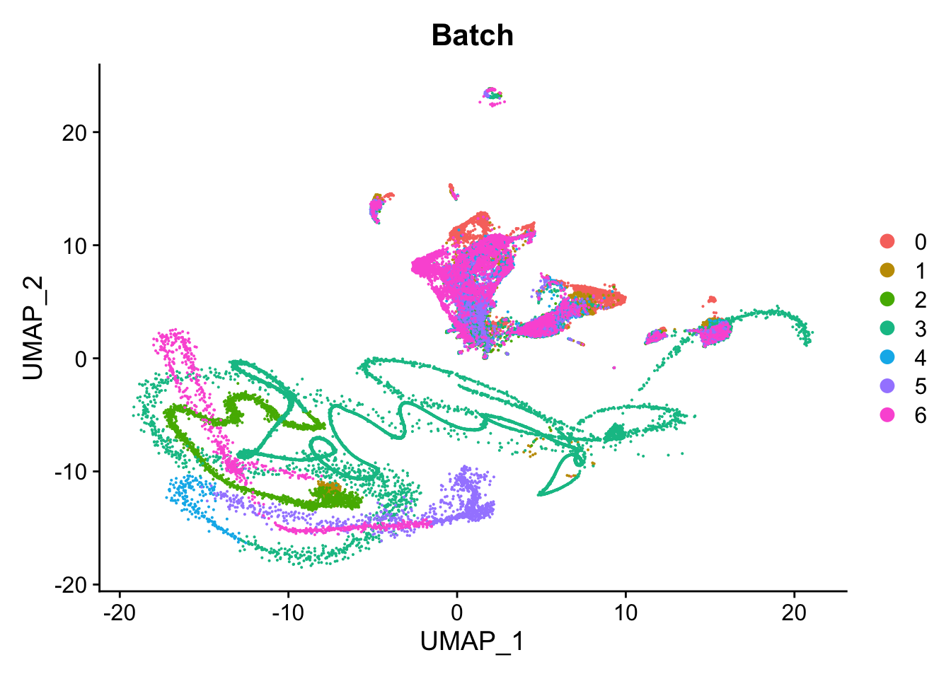 Strange cells primarily belong to the AT1 and Secretory lineages based
on
Strange cells primarily belong to the AT1 and Secretory lineages based
on Azimuth annotation.
DimPlot(seu, group.by = "predicted.ann_level_3", reduction = "umap")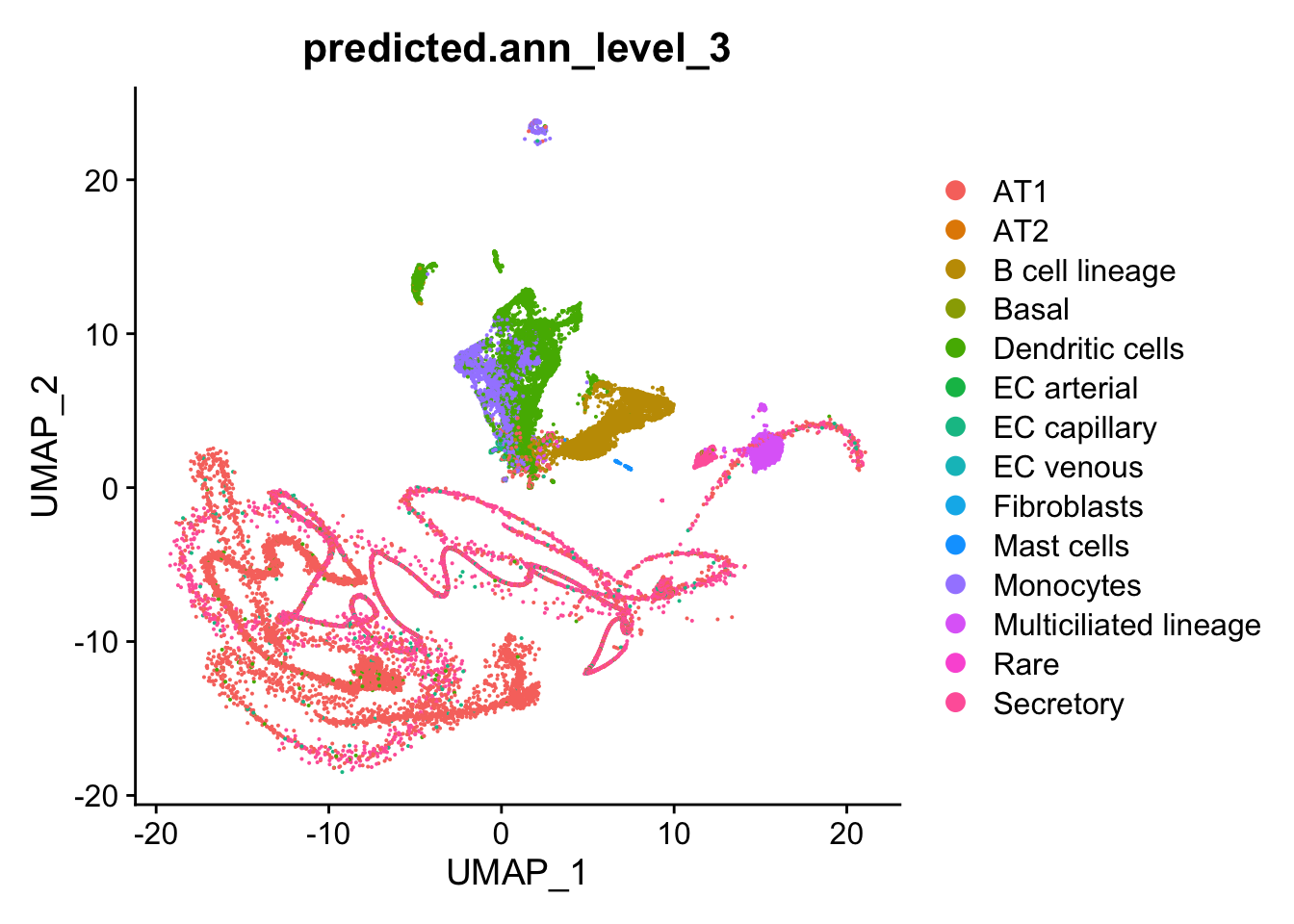
Examine cell library sizes after ambient removal per sample and per cell type. Some cells have very low library sizes after ambient removal.
VlnPlot(seu, features = "nCount_RNA", group.by = "sample.id", log = TRUE) +
  NoLegend() +
  geom_hline(yintercept = 250) +
  theme(axis.text = element_text(size = 10))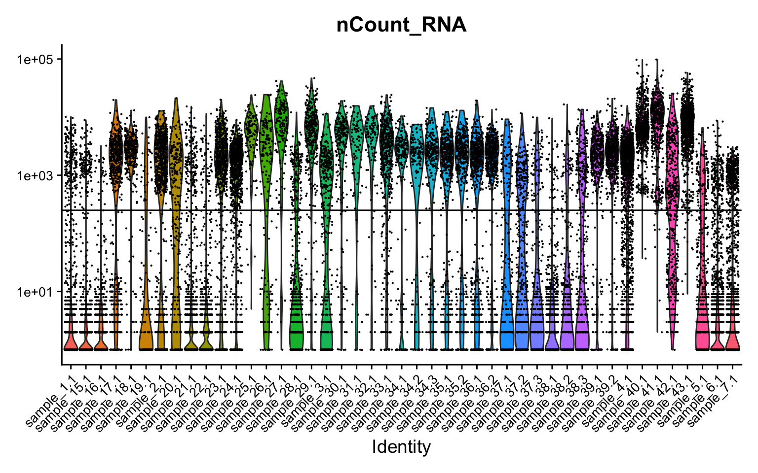
VlnPlot(seu, features = "nCount_RNA", group.by = "predicted.ann_level_3", log = TRUE) +
NoLegend() +
geom_hline(yintercept = 250) +
theme(axis.text = element_text(size = 10))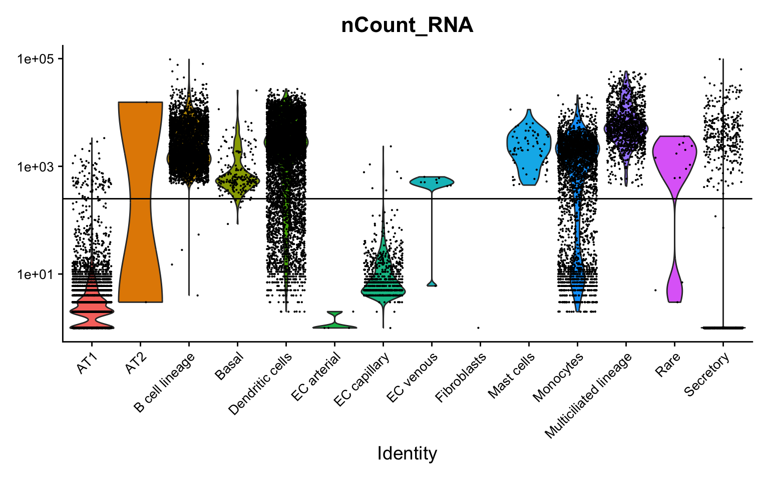 Filter our low library size cells and redo UMAP.
# remove low library size cells
seu <- subset(seu, cells = which(seu$nCount_RNA > 250))

seu <- ScaleData(seu) %>%
  FindVariableFeatures() %>%
  RunPCA(dims = 1:30, verbose = FALSE) %>%
  RunUMAP(dims = 1:30, verbose = FALSE)

DimPlot(seu, group.by = "Batch", reduction = "umap")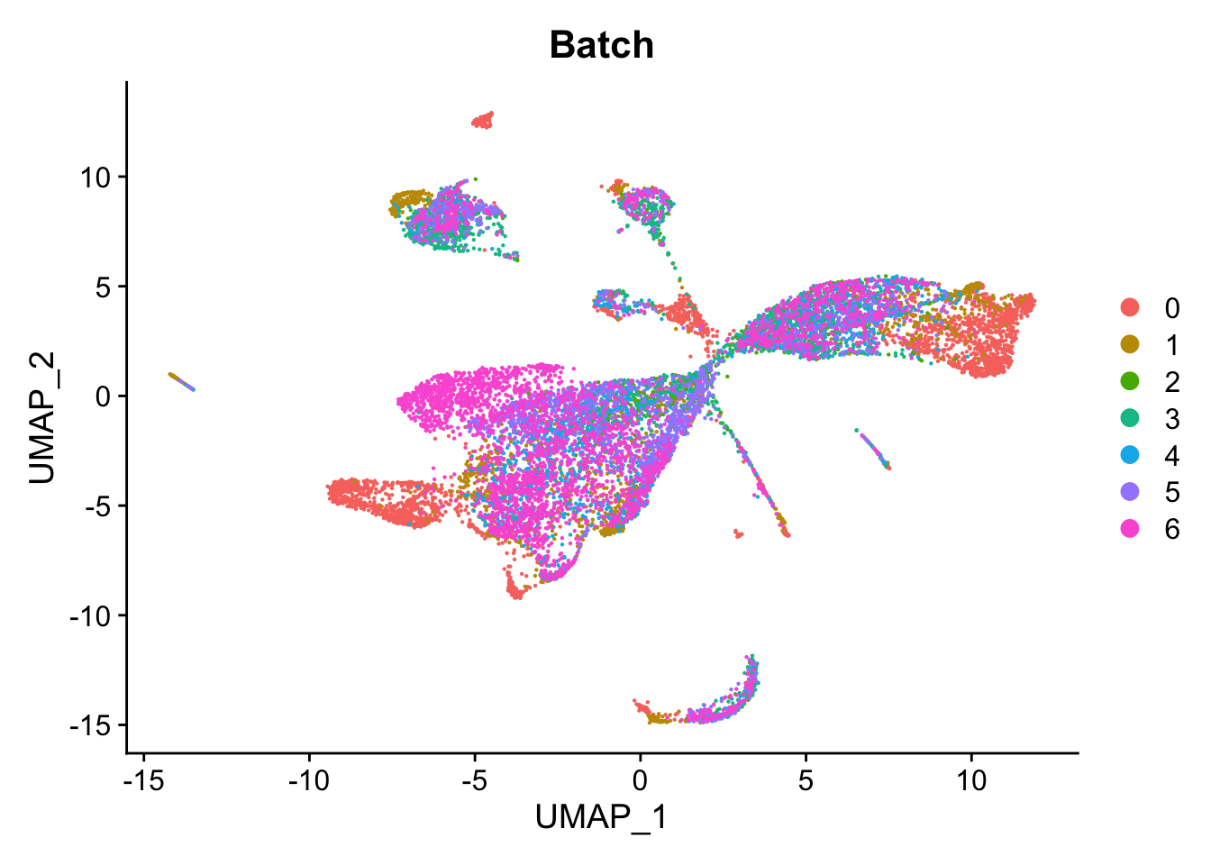
Cell cycle effect
Assign each cell a score, based on its expression of G2/M and S phase markers as described in the Seurat workflow here.
s.genes <- cc.genes.updated.2019$s.genes
g2m.genes <- cc.genes.updated.2019$g2m.genes

seu <- CellCycleScoring(seu, s.features = s.genes, g2m.features = g2m.genes,
                        set.ident = TRUE)
PCA of cell cycle genes.
DimPlot(seu, group.by = "Phase") -> p1

seu %>%
  RunPCA(features = c(s.genes, g2m.genes),
                      dims = 1:30, verbose = FALSE) %>%
  DimPlot(reduction = "pca") -> p2

(p2 / p1) + plot_layout(guides = "collect")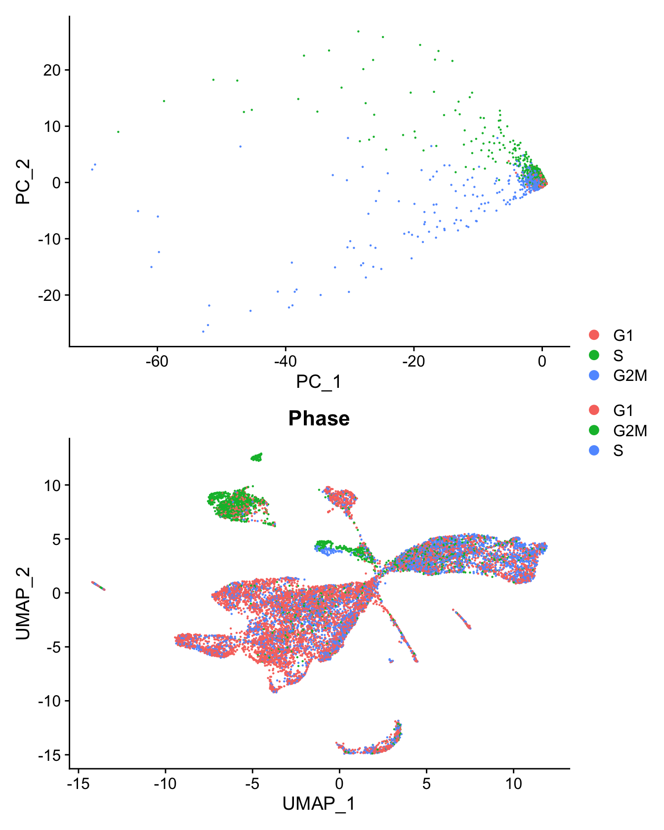
Distribution of cell cycle markers.
# Visualize the distribution of cell cycle markers across
RidgePlot(seu, features = c("PCNA", "TOP2A", "MCM6", "MKI67"), ncol = 2,
          log = TRUE)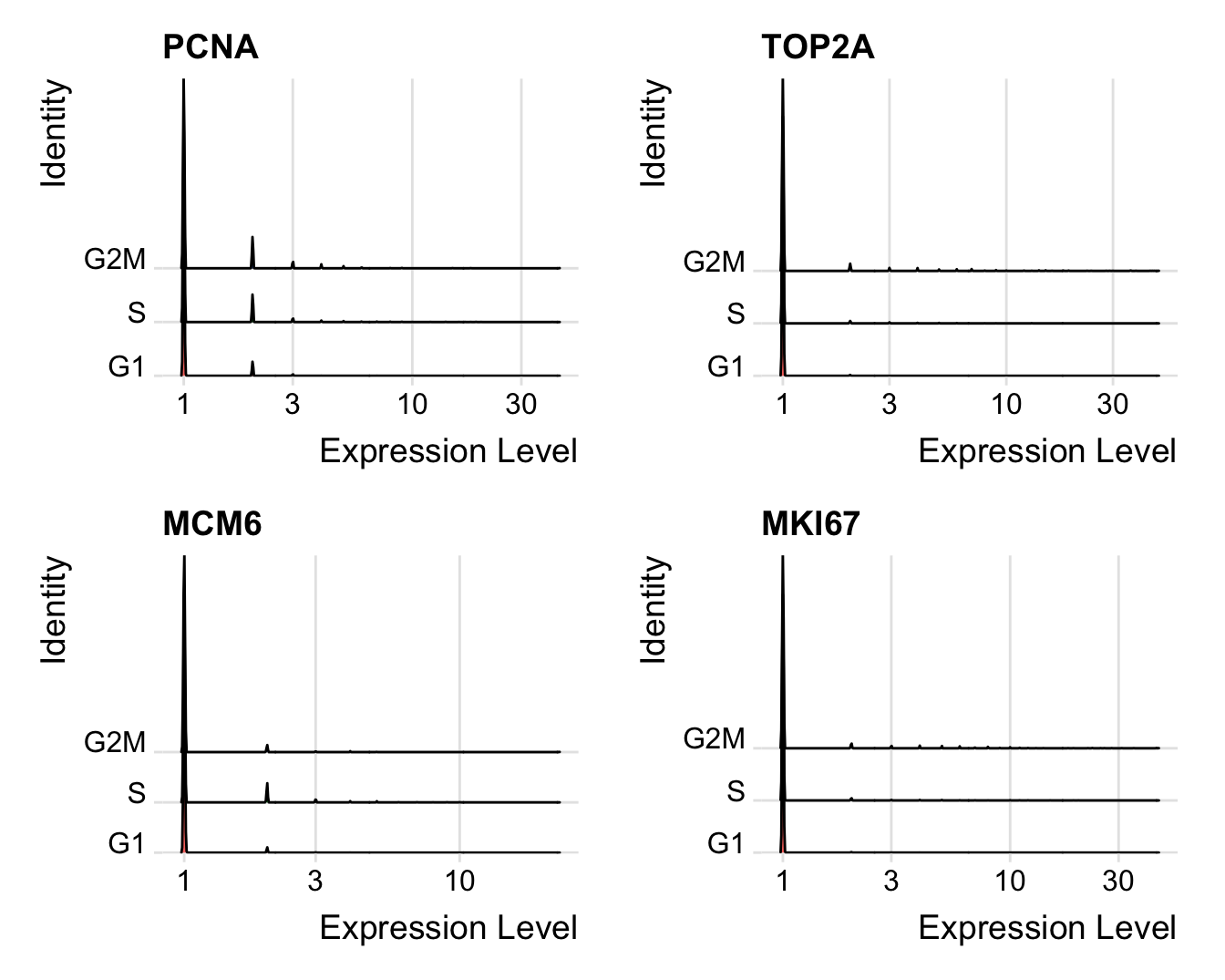
Using the Seurat Alternate Workflow from here,
calculate the difference between the G2M and S phase scores so that
signals separating non-cycling cells and cycling cells will be
maintained, but differences in cell cycle phase among proliferating
cells (which are often uninteresting), can be regressed out of the
data.
seu$CC.Difference <- seu$S.Score - seu$G2M.ScoreIntegrate RNA data
Split by batch for integration. Normalise with
SCTransform. Increase the strength of alignment by
increasing k.anchor parameter to 20 as recommended in
Seurat Fast integration with RPCA vignette.
First, integrate the RNA data.
out <- here("data",
            "C133_Neeland_merged",
            glue("C133_Neeland_full_clean{ambient}_integrated_other_cells.SEU.rds"))

if(!file.exists(out)){
  DefaultAssay(seu) <- "RNA"
  VariableFeatures(seu) <- NULL
  seu[["pca"]] <- NULL
  seu[["umap"]] <- NULL

  seuLst <- SplitObject(seu, split.by = "Batch")
  rm(seu)
  gc()

  # normalise with SCTransform and regress out cell cycle score difference
  seuLst <- lapply(X = seuLst, FUN = SCTransform, method = "glmGamPoi",
                   vars.to.regress = "CC.Difference")
  # integrate RNA data
  features <- SelectIntegrationFeatures(object.list = seuLst,
                                        nfeatures = 3000)
  seuLst <- PrepSCTIntegration(object.list = seuLst, anchor.features = features)
  seuLst <- lapply(X = seuLst, FUN = RunPCA, features = features)
  anchors <- FindIntegrationAnchors(object.list = seuLst,
                                    normalization.method = "SCT",
                                    anchor.features = features,
                                    k.anchor = 20,
                                    dims = 1:30, reduction = "rpca")
  seu <- IntegrateData(anchorset = anchors,
                       k.weight = min(100, min(sapply(seuLst, ncol)) - 5),
                       normalization.method = "SCT",
                       dims = 1:30)

  DefaultAssay(seu) <- "integrated"
  seu <- RunPCA(seu, dims = 1:30, verbose = FALSE) %>%
    RunUMAP(dims = 1:30, verbose = FALSE)

  saveRDS(seu, file = out)
  fs::file_chmod(out, "664")
  if(any(str_detect(fs::group_ids()$group_name,
                    "oshlack_lab"))) fs::file_chown(out,
                                                    group_id = "oshlack_lab")

} else {
  seu <- readRDS(file = out)

}
Integrate ADT data
out <- here("data",
            "C133_Neeland_merged",
            glue("C133_Neeland_full_clean{ambient}_integrated_other_cells.ADT.SEU.rds"))

# get ADT meta data
read.csv(file = here("data",
                     "C133_Neeland_batch1",
                     "data",
                     "sample_sheets",
                     "ADT_features.csv")) -> adt_data
# cleanup ADT meta data
pattern <- "anti-human/mouse |anti-human/mouse/rat |anti-mouse/human "
adt_data$name <- gsub(pattern, "", adt_data$name)
# change ADT rownames to antibody names
DefaultAssay(seu) <- "ADT"
if(all(rownames(seu[["ADT"]]@counts) == adt_data$id)){
  adt_counts <- seu[["ADT"]]@counts
  rownames(adt_counts) <- adt_data$name
  seu[["ADT"]] <- CreateAssayObject(counts = adt_counts)
}

if(!file.exists(out)){
  tmp <- DietSeurat(subset(seu, cells = which(seu$Batch != 0)),
                    assays = "ADT")
  DefaultAssay(tmp) <- "ADT"

  seuLst <- SplitObject(tmp, split.by = "Batch")
  seuLst <- lapply(X = seuLst, FUN = function(x) {
    # set all ADT as variable features
    VariableFeatures(x) <- rownames(x)
    x <- NormalizeData(x, normalization.method = "CLR", margin = 2)
    x
  })
  features <- SelectIntegrationFeatures(object.list = seuLst)
  seuLst <- lapply(X = seuLst, FUN = function(x) {
    x <- ScaleData(x, features = features, verbose = FALSE) %>%
      RunPCA(features = features, verbose = FALSE)
    x
  })
  anchors <- FindIntegrationAnchors(object.list = seuLst, reduction = "rpca",
                                    dims = 1:30)
  tmp <- IntegrateData(anchorset = anchors, dims = 1:30)

  DefaultAssay(tmp) <- "integrated"
  tmp <- ScaleData(tmp) %>%
    RunPCA(dims = 1:30, verbose = FALSE) %>%
    RunUMAP(dims = 1:30, verbose = FALSE)

  # create combined object that only contains cells with RNA+ADT data
  seuADT <- subset(seu, cells = which(seu$Batch !=0))
  seuADT[["integrated.adt"]] <- tmp[["integrated"]]
  seuADT[["pca.adt"]] <- tmp[["pca"]]
  seuADT[["umap.adt"]] <- tmp[["umap"]]

  saveRDS(seuADT, file = out)
  fs::file_chmod(out, "664")
  if(any(str_detect(fs::group_ids()$group_name,
                    "oshlack_lab"))) fs::file_chown(out,
                                                    group_id = "oshlack_lab")

} else {
  seuADT <- readRDS(file = out)

}
View integrated data
DefaultAssay(seuADT) <- "integrated"

DimPlot(seu, group.by = "Batch", reduction = "umap") -> p1
DimPlot(seuADT, group.by = "Batch", reduction = "umap") -> p2
DimPlot(seuADT, group.by = "Batch", reduction = "umap.adt") -> p3

(p1 / ((p2 | p3) +
  plot_layout(guides = "collect"))) &
  theme(axis.title = element_text(size = 8),
axis.text = element_text(size = 8)) 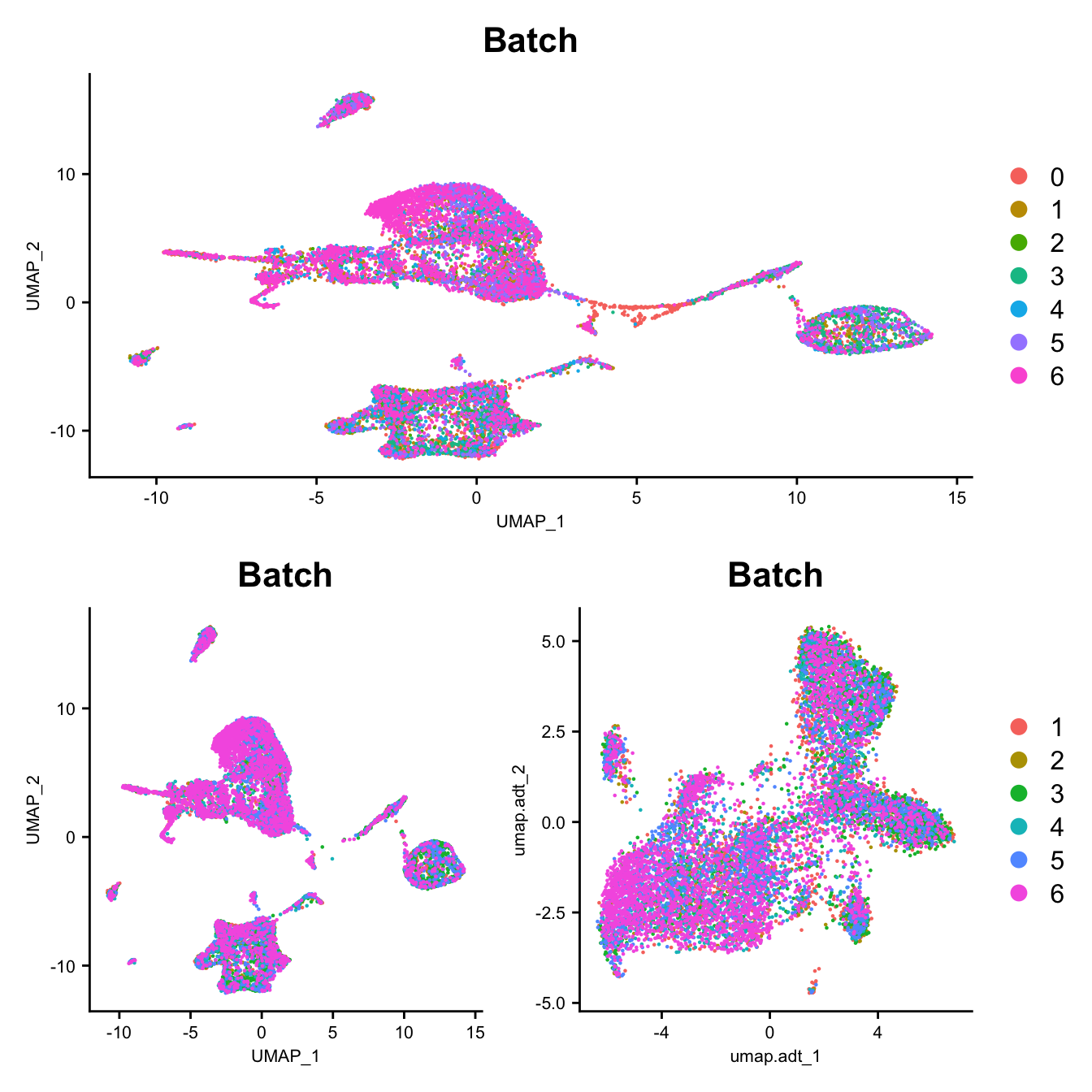
DimPlot(seu, group.by = "Phase", reduction = "umap") -> p1
DimPlot(seuADT, group.by = "Phase", reduction = "umap") -> p2
DimPlot(seuADT, group.by = "Phase", reduction = "umap.adt") -> p3

(p1 / ((p2 | p3) +
  plot_layout(guides = "collect"))) &
  theme(axis.title = element_text(size = 8),
axis.text = element_text(size = 8)) 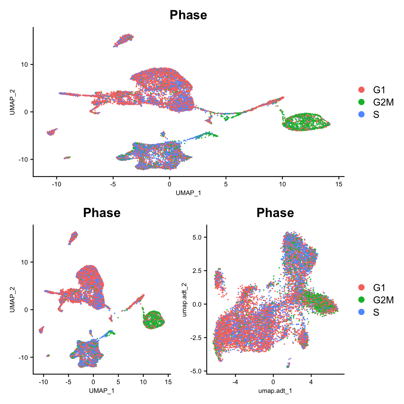
Cluster data
Perform clustering only on data that has ADT i.e. exclude batch 0.
Dimensionality reduction (RNA)
Exclude any mitochondrial, ribosomal, immunoglobulin and HLA genes from variable genes list, to encourage clustering by cell type.
# remove HLA, immunoglobulin, RNA, MT, and RP genes from variable genes list
var_regex = '^HLA-|^IG[HJKL]|^RNA|^MT-|^RP'
hvg <- grep(var_regex, VariableFeatures(seuADT), invert = TRUE, value = TRUE)
# assign edited variable gene list back to object
VariableFeatures(seuADT) <- hvg

# redo PCA and UMAP
seuADT <- RunPCA(seuADT, dims = 1:30, verbose = FALSE) %>%
    RunUMAP(dims = 1:30, verbose = FALSE)

DimHeatmap(seuADT, dims = 1:30, cells = 500, balanced = TRUE,
           reduction = "pca", assays = "integrated")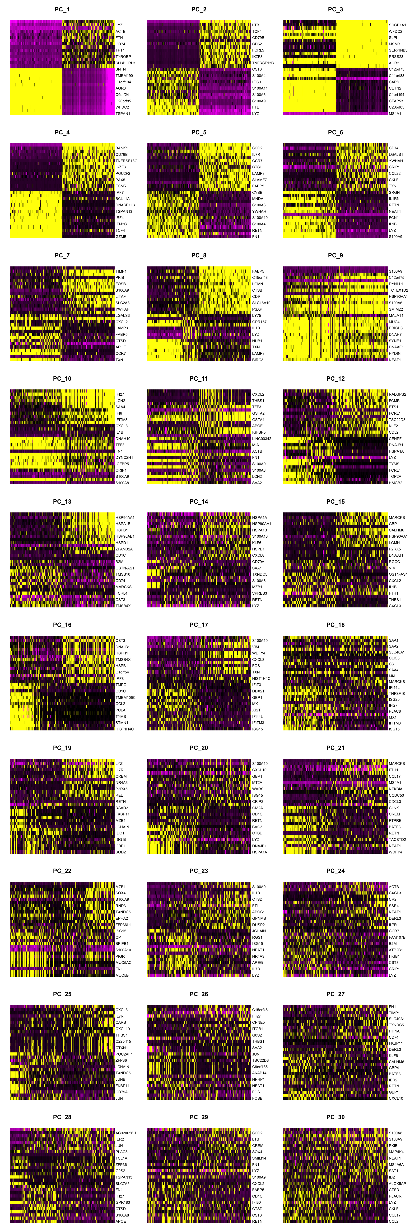
ElbowPlot(seuADT, ndims = 30, reduction = "pca")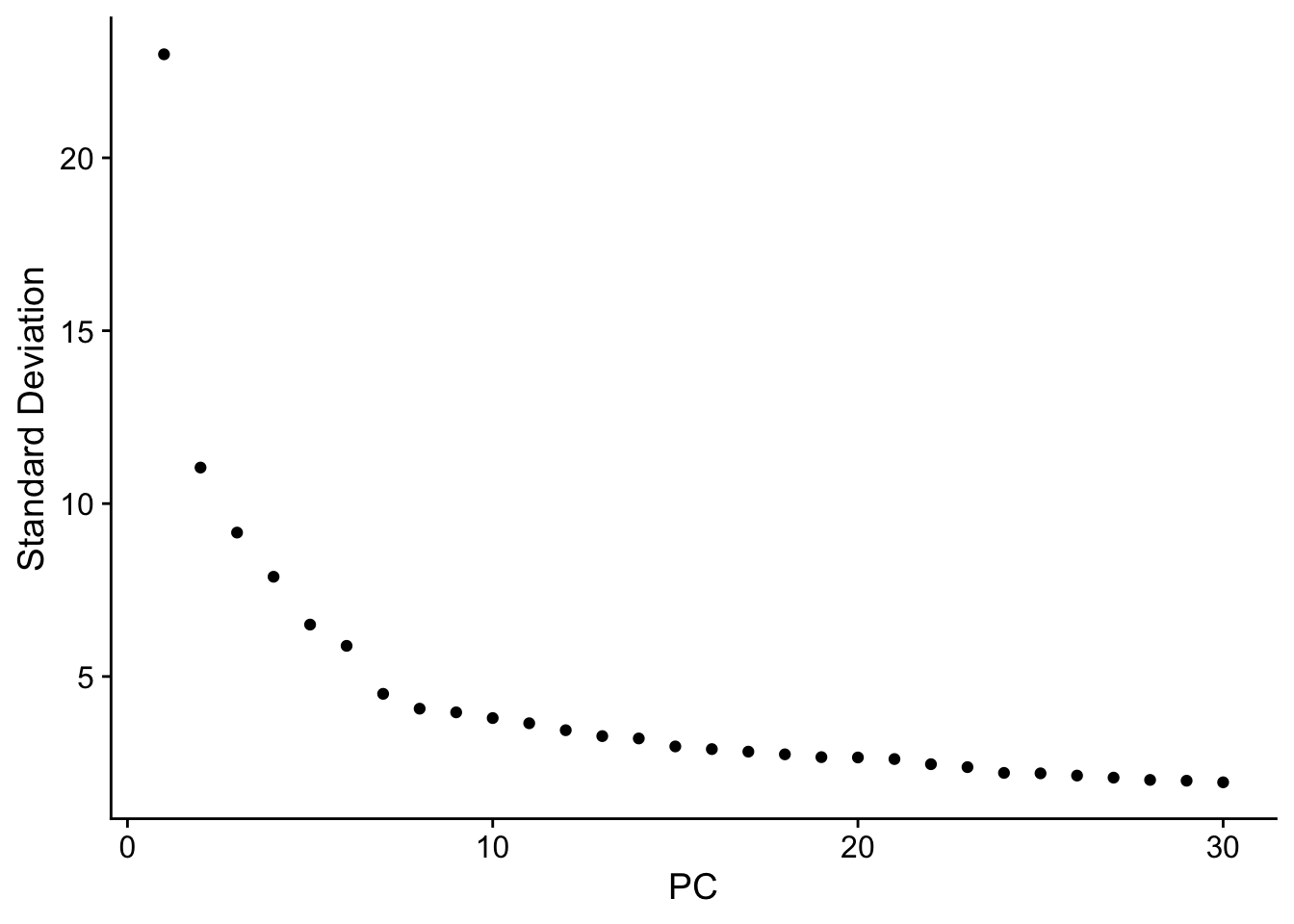
Dimensionality reduction (ADT)
DimHeatmap(seuADT, dims = 1:30, cells = 500, balanced = TRUE,
           reduction = "pca.adt", assays = "integrated.adt")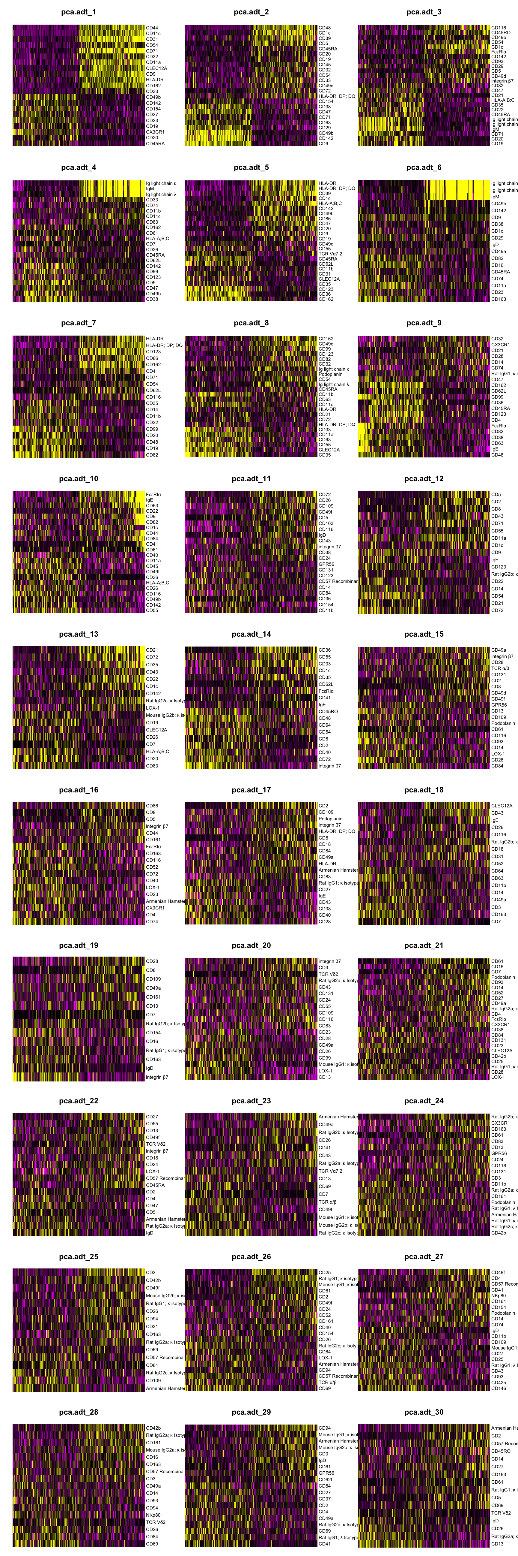
ElbowPlot(seuADT, ndims = 30, reduction = "pca.adt")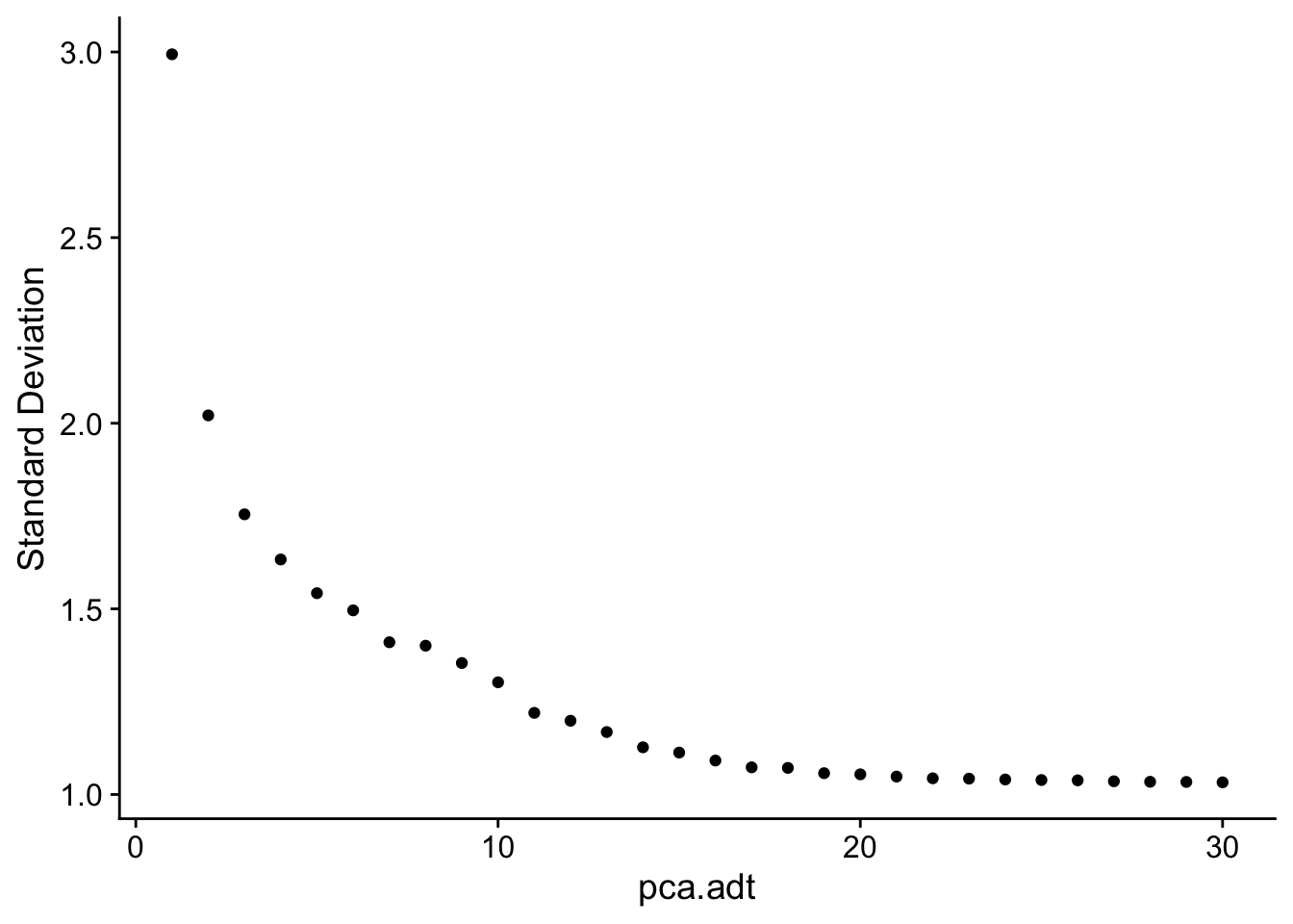
Run WNN clustering
Perform clustering at a range of resolutions and visualise to see which is appropriate to proceed with.
out <- here("data",
            "C133_Neeland_merged",
            glue("C133_Neeland_full_clean{ambient}_integrated_clustered_other_cells.ADT.SEU.rds"))

if(!file.exists(out)){
  DefaultAssay(seuADT) <- "integrated"
  seuADT <- FindMultiModalNeighbors(seuADT, reduction.list = list("pca", "pca.adt"),
                                 dims.list = list(1:30, 1:10),
                                 modality.weight.name = "RNA.weight")
  seuADT <- FindClusters(seuADT, algorithm = 3,
                      resolution = seq(0.1, 1, by = 0.1),
                      graph.name = "wsnn")
  seuADT <- RunUMAP(seuADT, dims = 1:30, nn.name = "weighted.nn",
                 reduction.name = "wnn.umap", reduction.key = "wnnUMAP_",
                 return.model = TRUE)
  saveRDS(seuADT, file = out)
  fs::file_chmod(out, "664")
  if(any(str_detect(fs::group_ids()$group_name,
                    "oshlack_lab"))) fs::file_chown(out,
                                                    group_id = "oshlack_lab")

} else {
  seuADT <- readRDS(file = out)

}

clustree::clustree(seuADT, prefix = "wsnn_res.")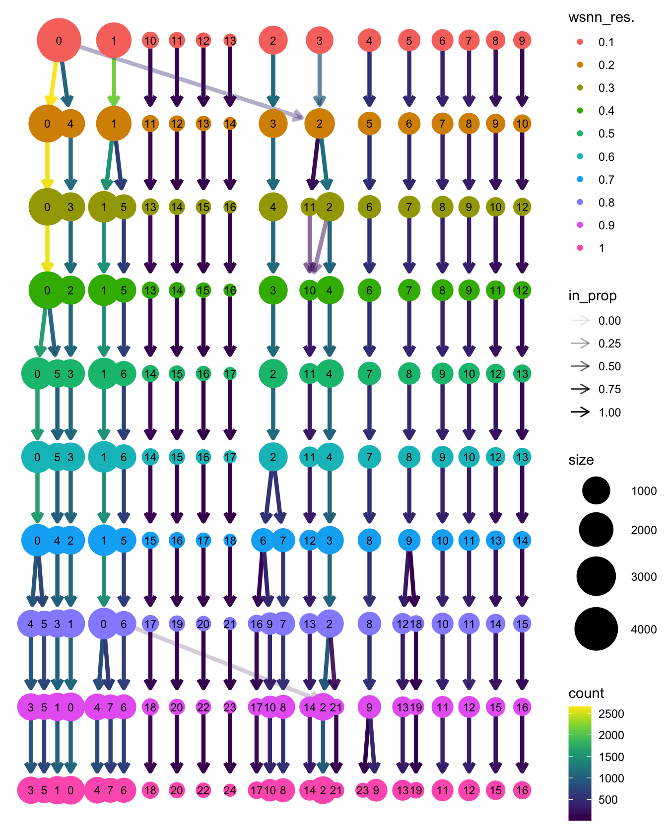
View clusters
Choose most appropriate resolution based on clustree
plot above.
grp <- "wsnn_res.0.6"
# change factor ordering
seuADT@meta.data[,grp] <- fct_inseq(seuADT@meta.data[,grp])

DimPlot(seuADT, group.by = grp, label = T) +
  theme(legend.position = "bottom")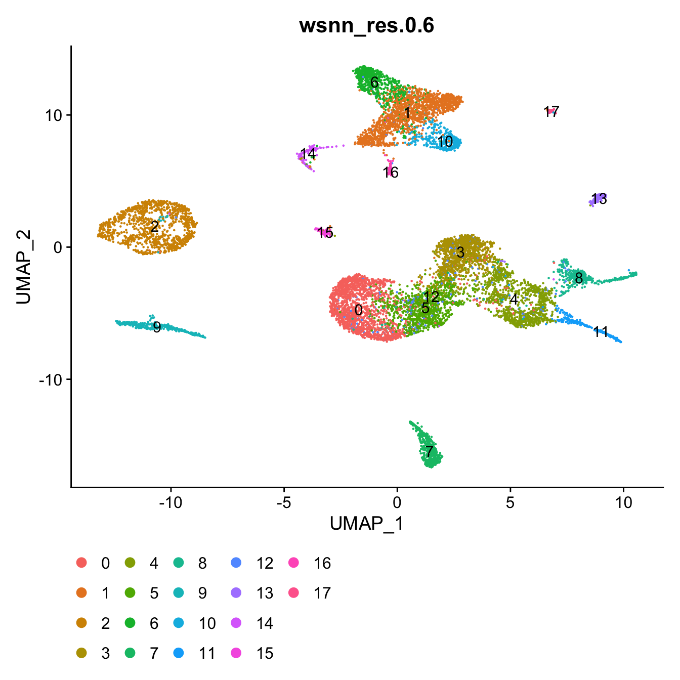
Weighting of RNA and ADT data per cluster.
 VlnPlot(seuADT, features = "integrated.weight", group.by = grp, sort = TRUE,
         pt.size = 0.1) +
  NoLegend()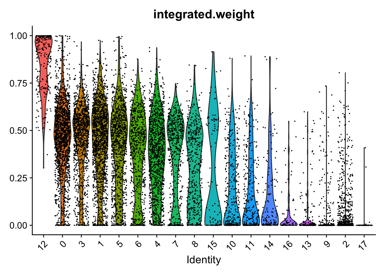
Reference mapping
Batch 0 only has RNA data and was not included in the WNN clustering of batched 1-6. To add this data we will map it to the WNN clustered reference.
Map data
Find transfer anchors.
# use WNN clustered batches 1-6 as reference
reference <- seuADT
DefaultAssay(seu) <- "RNA"
# batch 0 RNA data is the query
query <- DietSeurat(subset(seu, cells = which(seu$Batch == 0)),
                    assays = "RNA")

DefaultAssay(reference) <- "integrated"

anchors <- FindTransferAnchors(
  reference = reference,
  query = query,
  normalization.method = "SCT",
  reference.reduction = "pca",
  dims = 1:50
)
Map batch 0 samples onto reference.
query <- MapQuery(
  anchorset = anchors,
  query = query,
  reference = reference,
  refdata = list(
    wsnn = grp,
    ADT = "ADT"
  ),
  reference.reduction = "pca",
  reduction.model = "wnn.umap"
)

query
An object of class Seurat
20154 features across 2886 samples within 3 assays
Active assay: RNA (19973 features, 0 variable features)
2 other assays present: prediction.score.wsnn, ADT
2 dimensional reductions calculated: ref.pca, ref.umapVisualise batch 0 samples on reference UMAP.
query$predicted.wsnn <- fct_inseq(query$predicted.wsnn)

DimPlot(query, reduction = "ref.umap", group.by = "predicted.wsnn",
        label = TRUE, label.size = 3 ,repel = TRUE) +
  theme(legend.position = "bottom")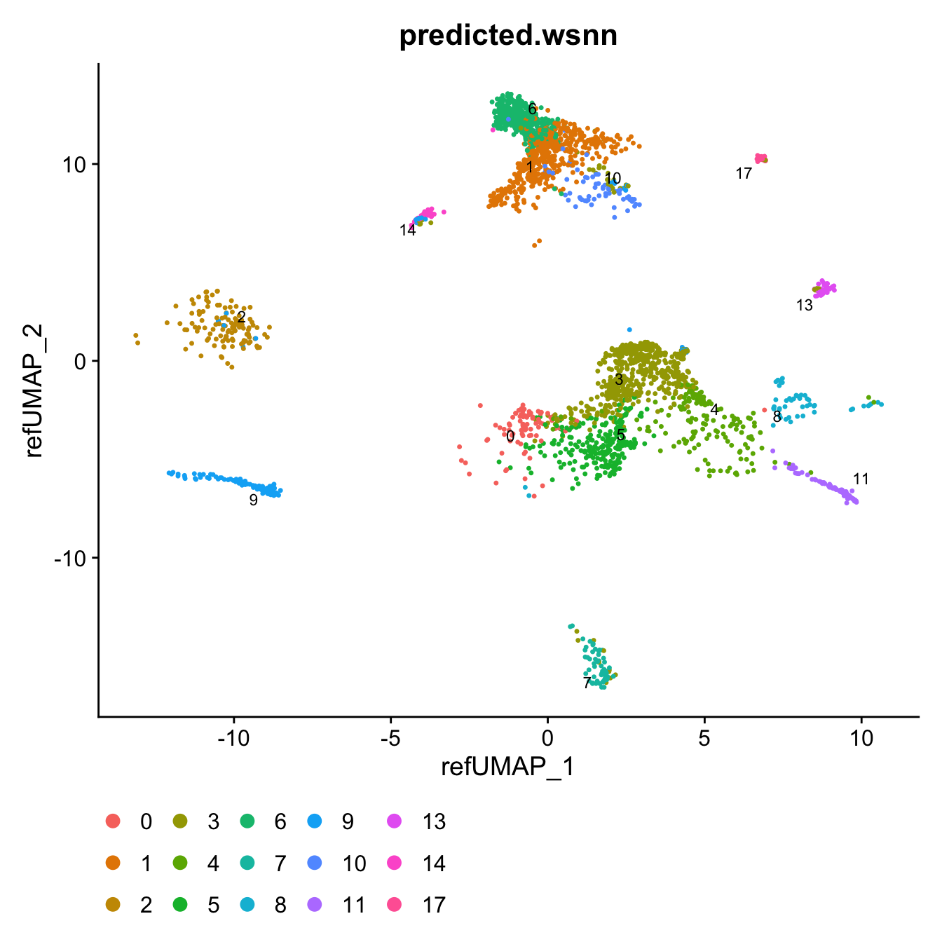
Distribution of Azimuth prediction scores per WNN
cluster.
ggplot(query@meta.data, aes(x = predicted.wsnn,
                            y = predicted.wsnn.score,
                            fill = predicted.wsnn)) +
  geom_boxplot() + NoLegend()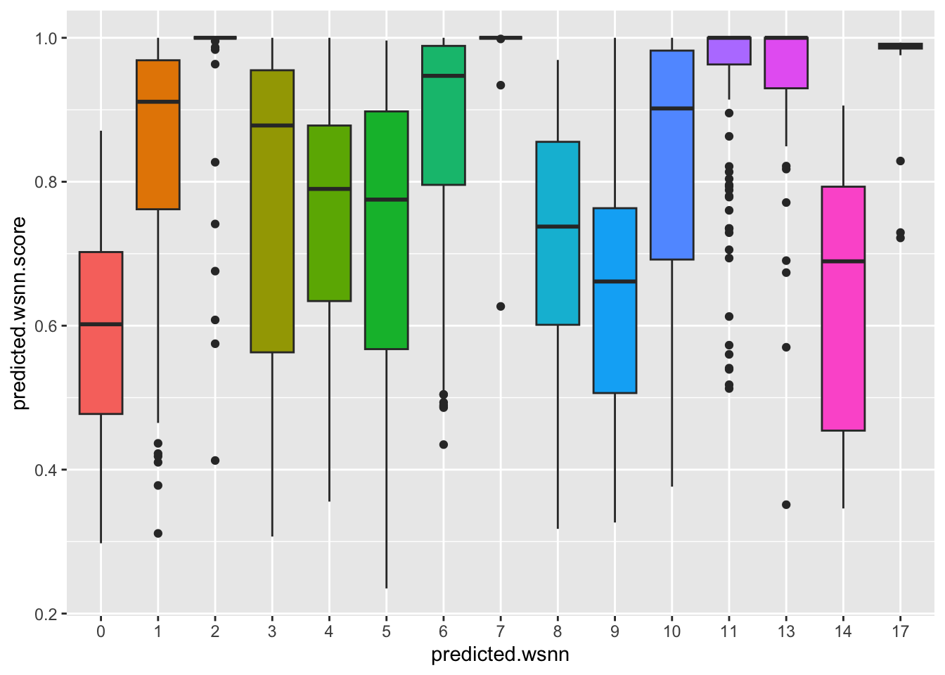
Compute combined UMAP
Computing a new UMAP can help to identify any cell states present in the query but not reference.
# merge reference (integrated + WNN clustered) and query (RNA only samples)
reference$id <- 'reference'
query$id <- 'query'
DefaultAssay(reference) <- "integrated"
refquery <- merge(DietSeurat(reference,
                             assays = c("RNA","ADT","integrated","SCT"),
                             dimreducs = c("pca")),
                  DietSeurat(query,
                             assays = c("RNA"),
                             dimreducs = "ref.pca"))
refquery[["pca"]] <- merge(reference[["pca"]], query[["ref.pca"]])
refquery <- RunUMAP(refquery, reduction = 'pca', dims = 1:50, assay = "integrated")
View combined UMAP.
# combine cluster annotations from reference and query
refquery@meta.data[, grp] <- ifelse(is.na(refquery@meta.data[,grp]),
                          refquery$predicted.wsnn,
                          refquery@meta.data[,grp])
# change factor ordering
refquery@meta.data[,grp] <- fct_inseq(refquery@meta.data[,grp])

DimPlot(refquery, reduction = "umap", group.by = grp,
label = TRUE, label.size = 3) + NoLegend() 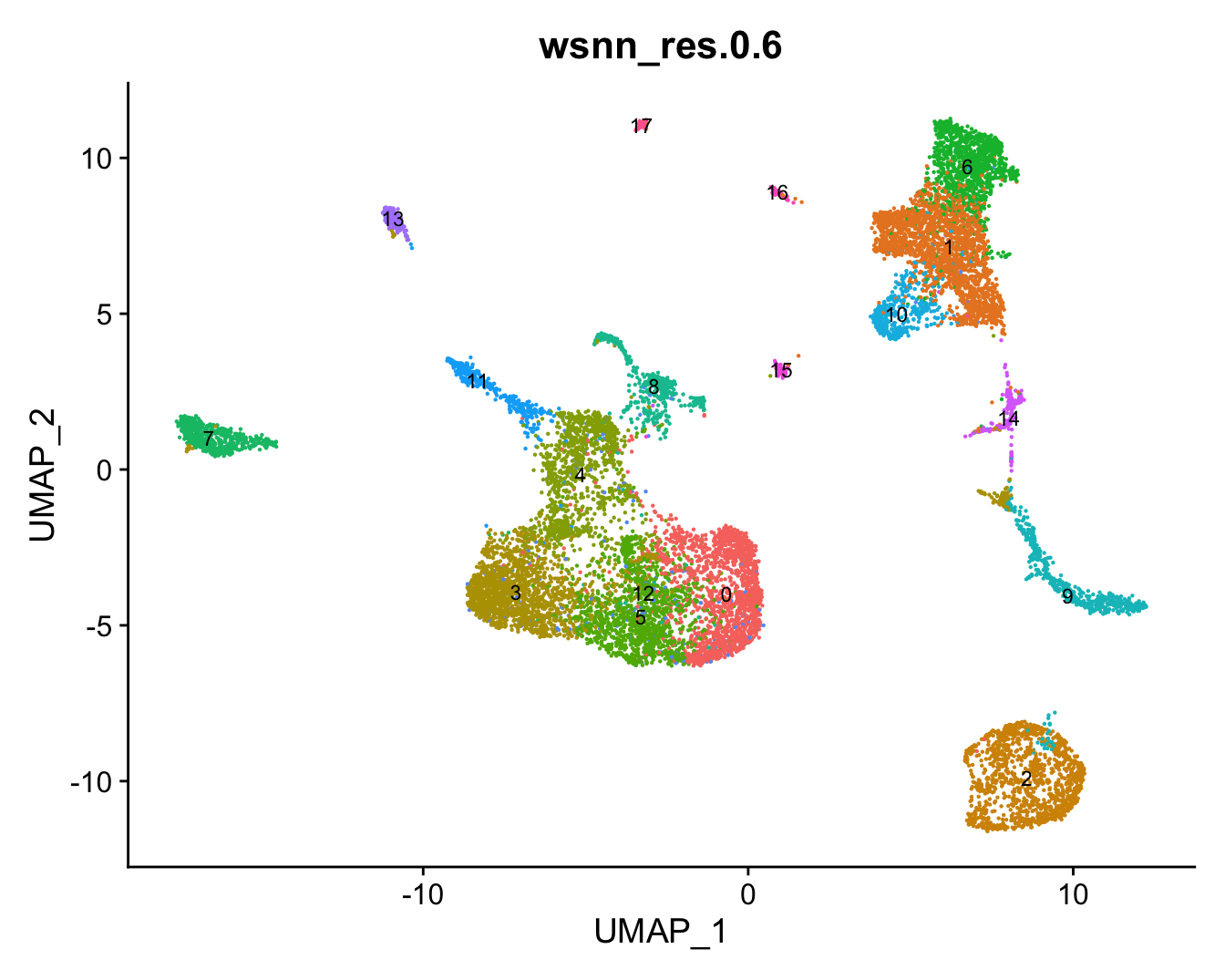
DimPlot(refquery, reduction = "umap", group.by = "Phase",
             label = FALSE, label.size = 3)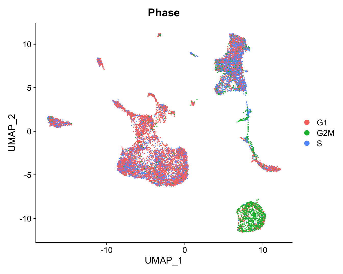
DimPlot(refquery, reduction = "umap", group.by = "Disease",
             label = FALSE, label.size = 3)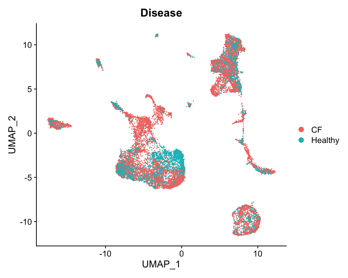
Save results.
out <- here("data",
            "C133_Neeland_merged",
            glue("C133_Neeland_full_clean{ambient}_integrated_clustered_mapped_other_cells.ADT.SEU.rds"))
if(!file.exists(out)){
  saveRDS(refquery, file = out)
  fs::file_chmod(out, "664")
  if(any(str_detect(fs::group_ids()$group_name,
                    "oshlack_lab"))) fs::file_chown(out,
                                                    group_id = "oshlack_lab")
}
Examine combined clusters
Number of cells per cluster.
refquery@meta.data %>%
  ggplot(aes(x = !!sym(grp), fill = !!sym(grp))) +
  geom_bar() +
  geom_text(aes(label = ..count..), stat = "count",
            vjust = -0.5, colour = "black", size = 2) +
  theme(axis.text.x = element_text(angle = 90, vjust = 0.5, hjust = 1)) +
  NoLegend()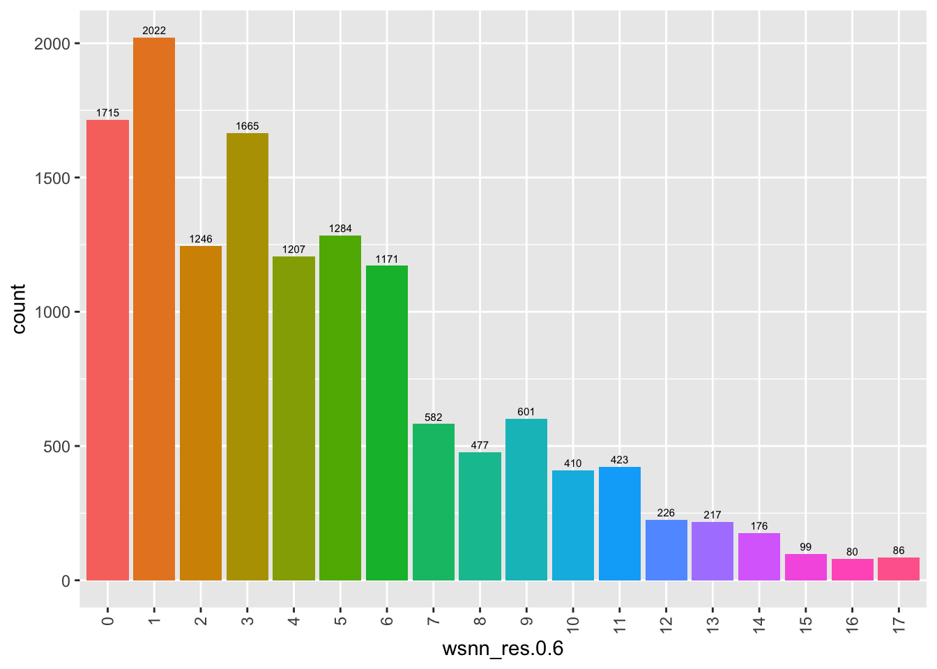
Visualise quality metrics by cluster. Cluster 17 potentially contains low quality cells.
refquery@meta.data %>%
  ggplot(aes(x = !!sym(grp),
             y = nCount_RNA,
             fill = !!sym(grp))) +
  geom_violin(scale = "area") +
  scale_y_log10() +
  NoLegend() -> p2

refquery@meta.data %>%
  ggplot(aes(x = !!sym(grp),
             y = nFeature_RNA,
             fill = !!sym(grp))) +
  geom_violin(scale = "area") +
  scale_y_log10() +
  NoLegend() -> p3

(p2 / p3) & theme(text = element_text(size = 8))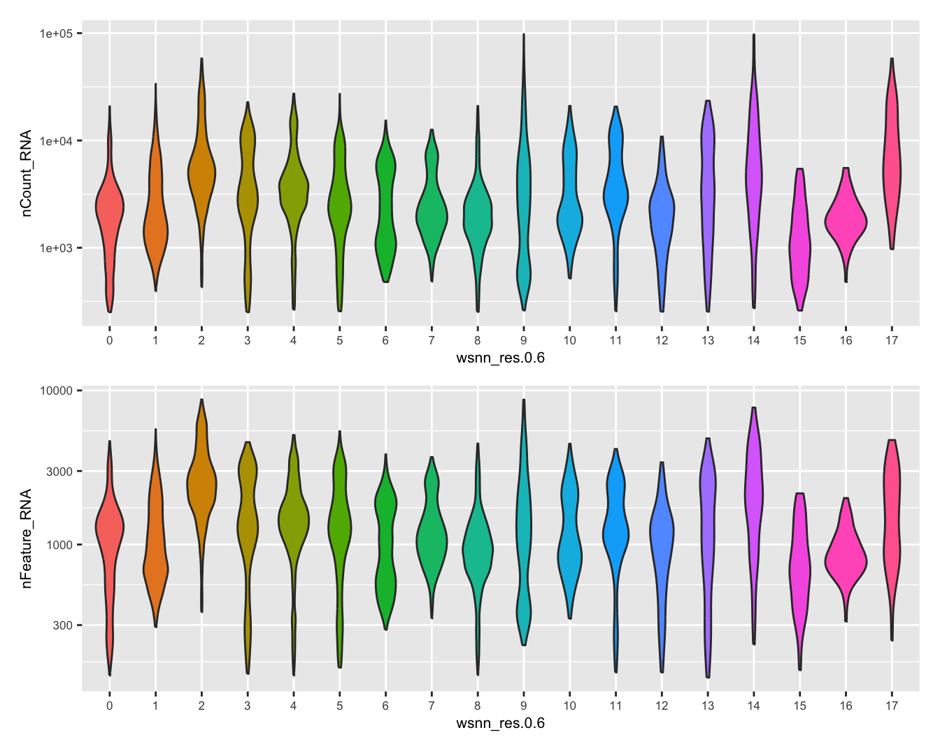
Check the batch composition of each of the clusters. Cluster 17 does not contain any cells from batch 0; could be a quality issue or the cell type was not captured in batch 0?
dittoBarPlot(refquery,
             var = "Batch",
             group.by = grp)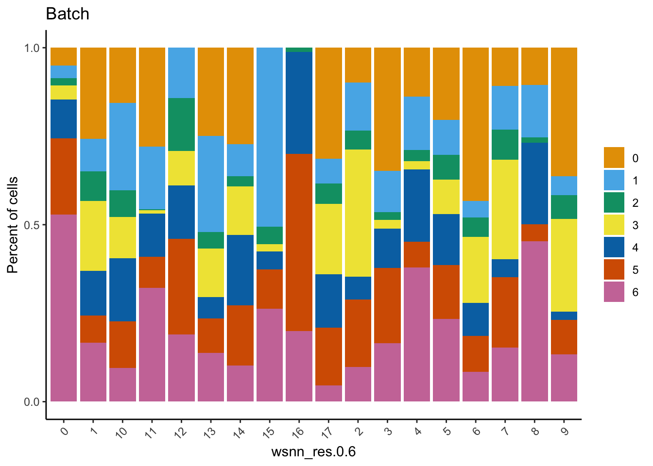
Check the sample compositions of combined clusters.
dittoBarPlot(refquery,
             var = "sample.id",
             group.by = grp) + ggtitle("Samples") +
  theme(legend.position = "bottom")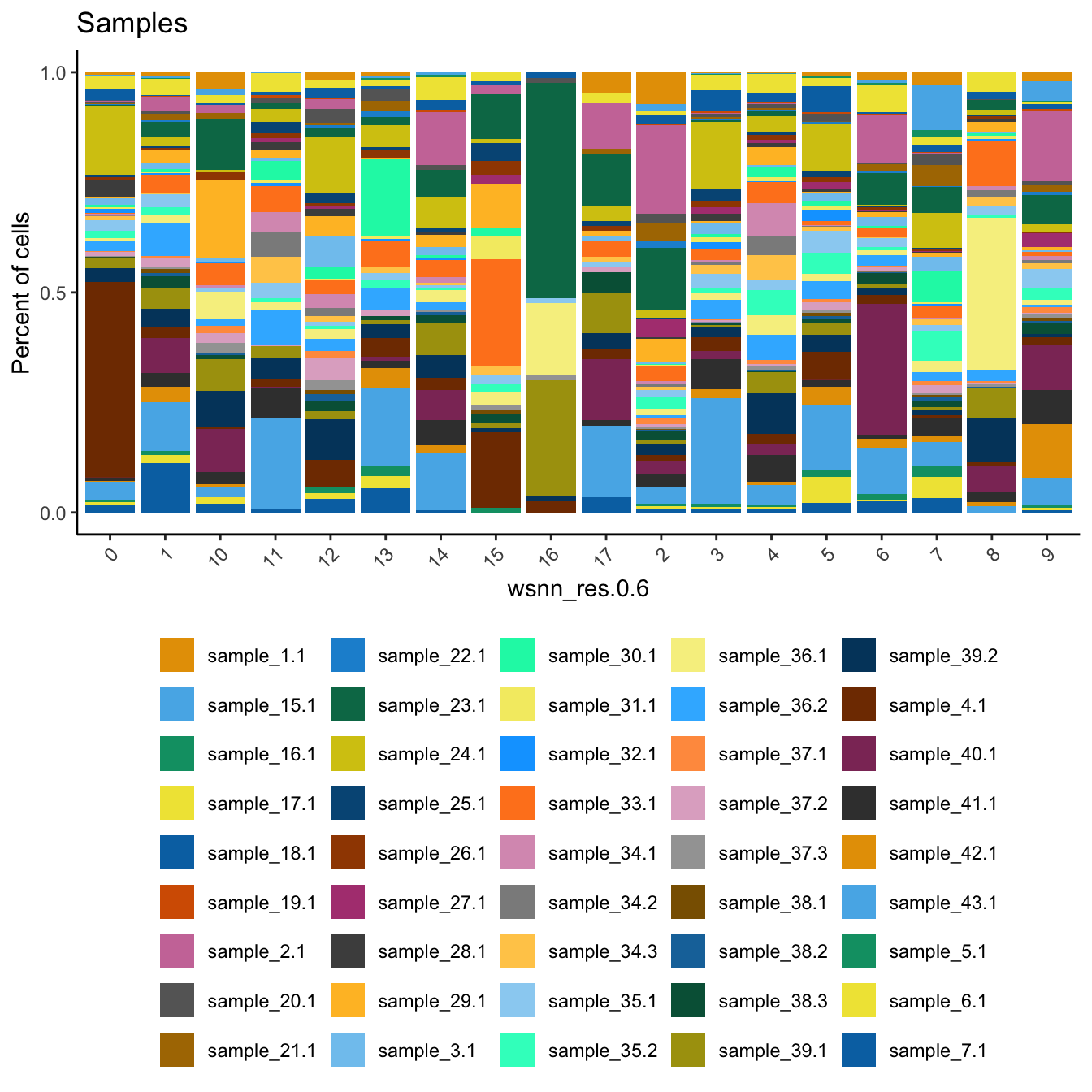
RNA marker gene analysis
Adapted from Dr. Belinda Phipson’s work for [@Sim2021-cg].
Test for marker genes using limma
# limma-trend for DE
Idents(refquery) <- grp

logcounts <- normCounts(DGEList(as.matrix(refquery[["RNA"]]@counts)),
                        log = TRUE, prior.count = 0.5)
entrez <- AnnotationDbi::mapIds(org.Hs.eg.db,
                                keys = rownames(logcounts),
                                column = c("ENTREZID"),
                                keytype = "SYMBOL",
                                multiVals = "first")
# remove genes without entrez IDs as these are difficult to interpret biologically
logcounts <- logcounts[!is.na(entrez),]
# remove confounding genes from counts table e.g. mitochondrial, ribosomal etc.
logcounts <- logcounts[!str_detect(rownames(logcounts), var_regex),]

maxclust <- length(levels(Idents(refquery))) - 1

clustgrp <- paste0("c", Idents(refquery))
clustgrp <- factor(clustgrp, levels = paste0("c", 0:maxclust))
donor <- factor(seu$sample.id)
batch <- factor(seu$Batch)

design <- model.matrix(~ 0 + clustgrp + donor)
colnames(design)[1:(length(levels(clustgrp)))] <- levels(clustgrp)

# Create contrast matrix
mycont <- matrix(NA, ncol = length(levels(clustgrp)),
                 nrow = length(levels(clustgrp)))
rownames(mycont) <- colnames(mycont) <- levels(clustgrp)
diag(mycont) <- 1
mycont[upper.tri(mycont)] <- -1/(length(levels(factor(clustgrp))) - 1)
mycont[lower.tri(mycont)] <- -1/(length(levels(factor(clustgrp))) - 1)

# Fill out remaining rows with 0s
zero.rows <- matrix(0, ncol = length(levels(clustgrp)),
                    nrow = (ncol(design) - length(levels(clustgrp))))
fullcont <- rbind(mycont, zero.rows)
rownames(fullcont) <- colnames(design)

fit <- lmFit(logcounts, design)

fit.cont <- contrasts.fit(fit, contrasts = fullcont)
fit.cont <- eBayes(fit.cont, trend = TRUE, robust = TRUE)

summary(decideTests(fit.cont))
c0 c1 c2 c3 c4 c5 c6 c7 c8 c9 c10 c11
Down 6833 5641 2658 5163 4286 4830 6262 2950 5699 3400 2837 4919
NotSig 7042 7509 4295 8311 8739 8162 7381 9228 8542 8486 10761 9255
Up 1747 2472 8669 2148 2597 2630 1979 3444 1381 3736 2024 1448
c12 c13 c14 c15 c16 c17
Down 1001 2609 389 1522 454 902
NotSig 13914 12145 12402 12448 14566 14072
Up 707 868 2831 1652 602 648Test relative to a threshold (TREAT).
tr <- treat(fit.cont, lfc = 0.25)
dt <- decideTests(tr)
summary(dt)
c0 c1 c2 c3 c4 c5 c6 c7 c8 c9 c10 c11
Down 91 261 343 57 35 66 412 170 115 403 162 141
NotSig 15212 15170 13362 15308 15177 15179 15042 15022 15182 14838 15279 15135
Up 319 191 1917 257 410 377 168 430 325 381 181 346
c12 c13 c14 c15 c16 c17
Down 12 83 29 247 68 157
NotSig 15473 15369 15208 15240 15465 15333
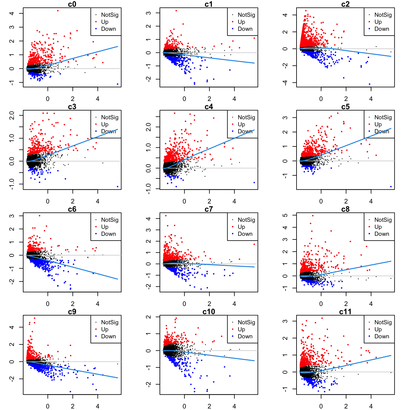
Up 137 170 385 135 89 132Mean-difference (MD) plots per cluster.
par(mfrow=c(4,3))
par(mar=c(2,3,1,2))

for(i in 1:ncol(mycont)){
  plotMD(tr, coef = i, status = dt[,i], hl.cex = 0.5)
  abline(h = 0, col = "lightgrey")
  lines(lowess(tr$Amean, tr$coefficients[,i]), lwd = 1.5, col = 4)
}
limma marker gene dotplot
DefaultAssay(refquery) <- "RNA"
contnames <- colnames(mycont)
top_markers <- NULL
n_markers <- 10

for(i in 1:ncol(mycont)){
  top <- topTreat(tr, coef = i, n = Inf)
  top <- top[top$logFC > 0, ]
  top_markers <- c(top_markers,
                   setNames(rownames(top)[1:n_markers],
                            rep(contnames[i], n_markers)))
}

top_markers <- top_markers[!is.na(top_markers)]
top_markers <- top_markers[!duplicated(top_markers)]
cols <- paletteer::paletteer_d("pals::glasbey")[factor(names(top_markers))]

DotPlot(refquery,
        features = unname(top_markers),
        group.by = grp,
        cols = c("azure1", "blueviolet"),
        dot.scale = 3, assay = "SCT") +
    RotatedAxis() +
    FontSize(y.text = 8, x.text = 12) +
    labs(y = element_blank(), x = element_blank()) +
    coord_flip() +
  theme(axis.text.y = element_text(color = cols)) +
  ggtitle("Top 10 cluster marker genes (no duplicates)")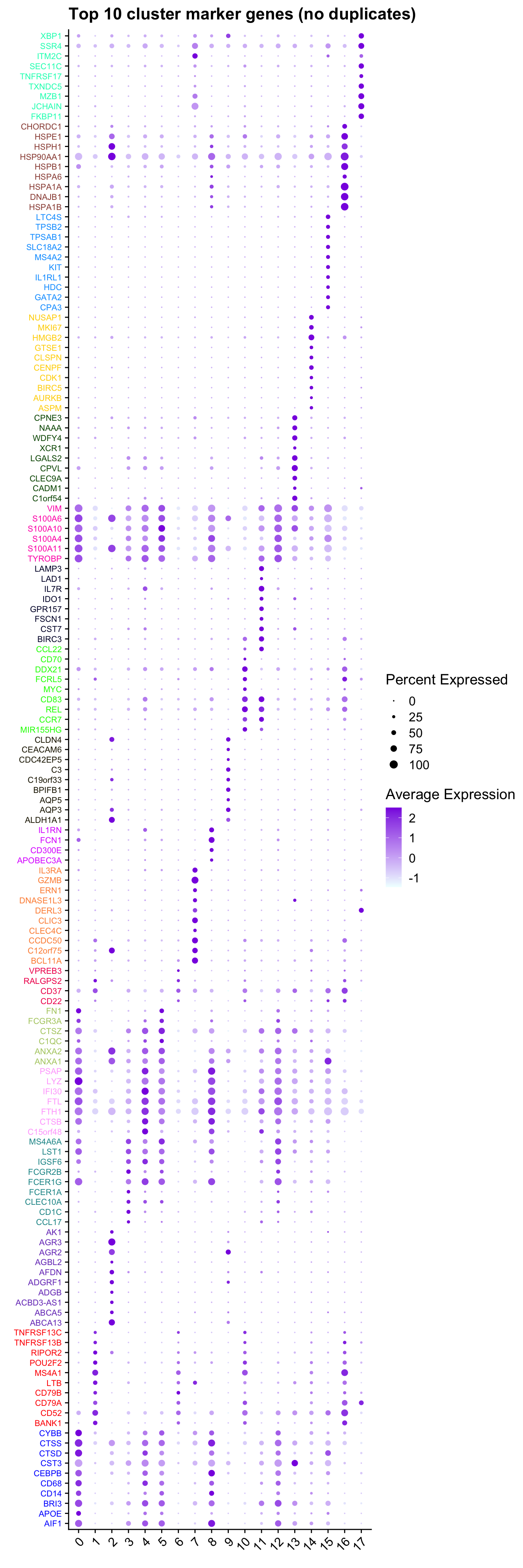
Save marker genes and pathways
The Broad MSigDB Reactome pathways are tested for each contrast using
cameraPR from limma. The cameraPR
method tests whether a set of genes is highly ranked relative to other
genes in terms of differential expression, accounting for inter-gene
correlation.
Prepare gene sets of interest.
if(!file.exists(here("data/Hs.c2.cp.reactome.v7.1.entrez.rds")))
  download.file("https://bioinf.wehi.edu.au/MSigDB/v7.1/Hs.c2.cp.reactome.v7.1.entrez.rds",
                here("data/Hs.c2.cp.reactome.v7.1.entrez.rds"))

Hs.c2.reactome <- readRDS(here("data/Hs.c2.cp.reactome.v7.1.entrez.rds"))

gns <- AnnotationDbi::mapIds(org.Hs.eg.db,
                             keys = rownames(tr),
                             column = c("ENTREZID"),
                             keytype = "SYMBOL",
                             multiVals = "first")
Run pathway analysis and save results to file.
options(scipen=-1, digits = 6)
contnames <- colnames(mycont)
dirName <- here("output",
                "cluster_markers",
                glue("RNA{ambient}"),
                "other_cells")

if(!dir.exists(dirName)) dir.create(dirName, recursive = TRUE)

for(c in colnames(tr)){
  top <- topTreat(tr, coef = c, n = Inf)
  top <- top[top$logFC > 0, ]

  write.csv(top[1:100, ] %>%
              rownames_to_column(var = "Symbol"),
            file = glue("{dirName}/up-cluster-limma-{c}.csv"),
            sep = ",",
            quote = FALSE,
            col.names = NA,
            row.names = TRUE)

  # get marker indices
  c2.id <- ids2indices(Hs.c2.reactome, unname(gns[rownames(tr)]))
  # gene set testing results
  cameraPR(tr$t[,glue("{c}")], c2.id) %>%
    rownames_to_column(var = "Pathway") %>%
    dplyr::filter(Direction == "Up") %>%
    slice_head(n = 50) %>%
    write.csv(file = here(glue("{dirName}/REACTOME-cluster-limma-{c}.csv")),
            sep = ",",
            quote = FALSE,
            col.names = NA,
            row.names = TRUE)
}
ADT marker analysis
Find all marker ADT using limma
# identify isotype controls for DSB ADT normalisation
read_csv(file = here("data",
                     "C133_Neeland_batch1",
                     "data",
                     "sample_sheets",
                     "ADT_features.csv")) %>%
  dplyr::filter(grepl("[Ii]sotype", name)) %>%
  pull(name) -> isotype_controls

# normalise ADT using DSB normalisation
adt <- seuADT[["ADT"]]@counts
adt_dsb <- ModelNegativeADTnorm(cell_protein_matrix = adt,
                                denoise.counts = TRUE,
                                use.isotype.control = TRUE,
                                isotype.control.name.vec = isotype_controls)
[1] "fitting models to each cell for dsb technical component and removing cell to cell technical noise"Running the limma analysis on the normalised counts.
# limma-trend for DE
Idents(seuADT) <- grp

logcounts <- adt_dsb
# remove isotype controls from marker analysis
logcounts <- logcounts[!rownames(logcounts) %in% isotype_controls,]
maxclust <- length(levels(Idents(seuADT))) - 1

clustgrp <- paste0("c", Idents(seuADT))
clustgrp <- factor(clustgrp, levels = paste0("c", 0:maxclust))
donor <- seuADT$sample.id

design <- model.matrix(~ 0 + clustgrp + donor)
colnames(design)[1:(length(levels(clustgrp)))] <- levels(clustgrp)

# Create contrast matrix
mycont <- matrix(NA, ncol = length(levels(clustgrp)),
                 nrow = length(levels(clustgrp)))
rownames(mycont) <- colnames(mycont) <- levels(clustgrp)
diag(mycont) <- 1
mycont[upper.tri(mycont)] <- -1/(length(levels(factor(clustgrp))) - 1)
mycont[lower.tri(mycont)] <- -1/(length(levels(factor(clustgrp))) - 1)

# Fill out remaining rows with 0s
zero.rows <- matrix(0, ncol = length(levels(clustgrp)),
                    nrow = (ncol(design) - length(levels(clustgrp))))
fullcont <- rbind(mycont, zero.rows)
rownames(fullcont) <- colnames(design)

fit <- lmFit(logcounts, design)
fit.cont <- contrasts.fit(fit, contrasts = fullcont)
fit.cont <- eBayes(fit.cont, trend = TRUE, robust = TRUE)

summary(decideTests(fit.cont))
c0 c1 c2 c3 c4 c5 c6 c7 c8 c9 c10 c11 c12 c13 c14 c15 c16 c17
Down 26 61 71 42 22 34 71 64 28 53 56 33 21 39 5 32 30 30
NotSig 75 58 61 77 76 73 57 69 73 75 75 84 89 92 123 98 118 113
Up 53 35 22 35 56 47 26 21 53 26 23 37 44 23 26 24 6 11Test relative to a threshold (TREAT).
tr <- treat(fit.cont, lfc = 0.1)
dt <- decideTests(tr)
summary(dt)
c0 c1 c2 c3 c4 c5 c6 c7 c8 c9 c10 c11 c12 c13 c14 c15 c16 c17
Down 8 34 39 15 4 8 38 31 9 26 33 9 3 17 1 16 13 9
NotSig 113 107 108 120 119 118 108 113 123 118 115 128 127 123 148 122 139 139
Up 33 13 7 19 31 28 8 10 22 10 6 17 24 14 5 16 2 6ADT marker dot plot
Dot plot of the top 5 ADT markers per cluster without duplication.
contnames <- colnames(mycont)
top_markers <- NULL
n_markers <- 5

for (i in 1:length(contnames)){
  top <- topTreat(tr, coef = i, n = Inf)
  top <- top[top$logFC > 0,]
  top_markers <- c(top_markers,
                   setNames(rownames(top)[1:n_markers],
                            rep(contnames[i], n_markers)))
}

top_markers <- top_markers[!is.na(top_markers)]
top_markers <- top_markers[!duplicated(top_markers)]
cols <- paletteer::paletteer_d("pals::glasbey")[factor(names(top_markers))][!duplicated(top_markers)]

# add DSB normalised data to Seurat assay for plotting
seuADT[["ADT.dsb"]] <- CreateAssayObject(data = logcounts)
DotPlot(seuADT,
        group.by = grp,
        features = unname(top_markers),
        cols = c("azure1", "blueviolet"),
        assay = "ADT.dsb")  +
  RotatedAxis() +
  FontSize(y.text = 8, x.text = 9) +
  labs(y = element_blank(), x = element_blank()) +
  theme(axis.text.y = element_text(color = cols),
        legend.text = element_text(size = 10),
        legend.title = element_text(size = 10)) +
    coord_flip() +
  ggtitle("Top 5 cluster markers ADTs (no duplicates)")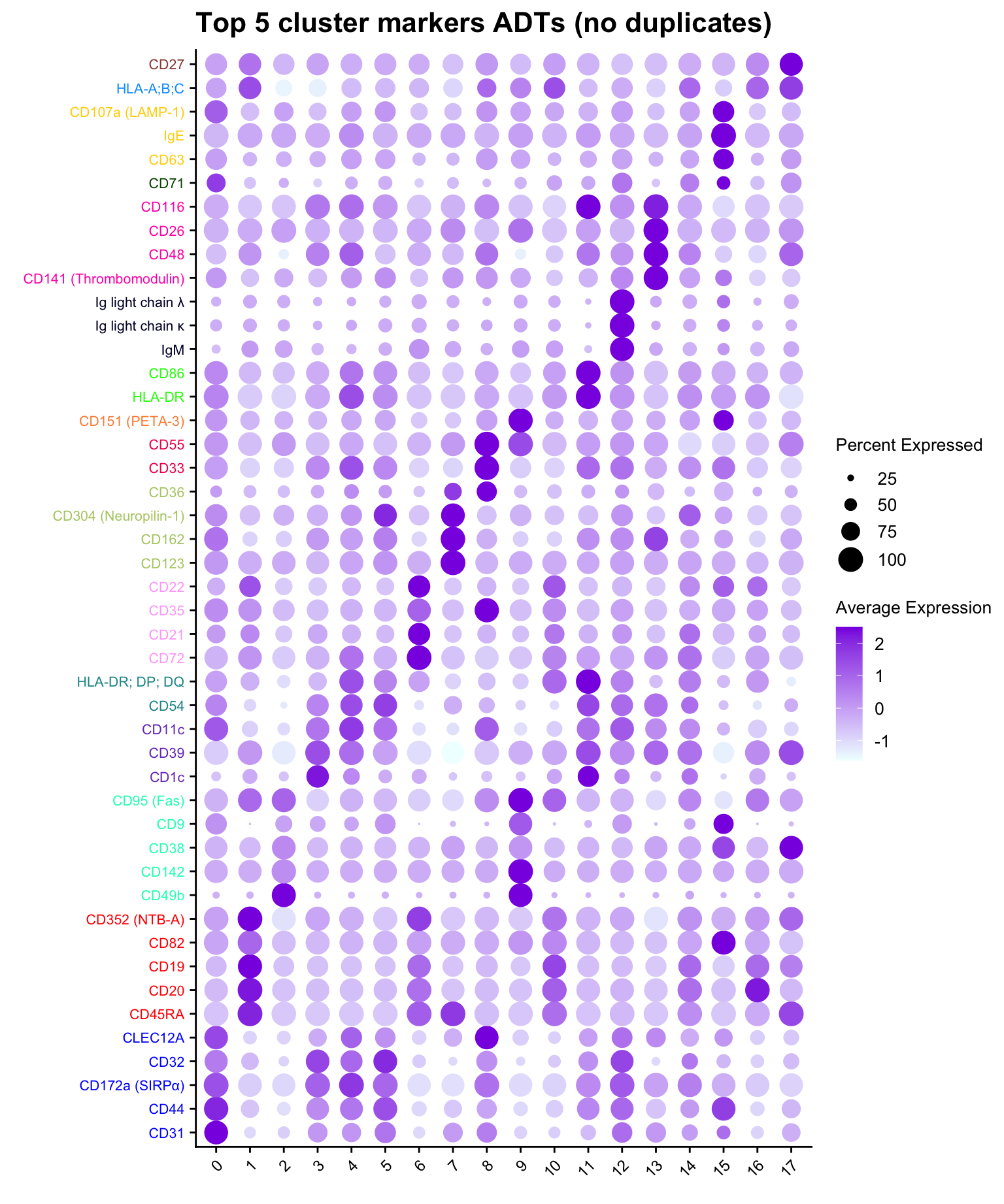
ADT marker heatmap
Make data frame of proteins, clusters, expression levels.
cbind(seuADT@meta.data %>%
        dplyr::select(!!sym(grp)),
      as.data.frame(t(seuADT@assays$ADT.dsb@data))) %>%
  rownames_to_column(var = "cell") %>%
  pivot_longer(c(-!!sym(grp), -cell),
               names_to = "ADT",
               values_to = "expression") %>%
  dplyr::group_by(!!sym(grp), ADT) %>%
  dplyr::summarize(Expression = mean(expression)) %>%
  ungroup() -> dat

# plot expression density to select heatmap colour scale range
plot(density(dat$Expression))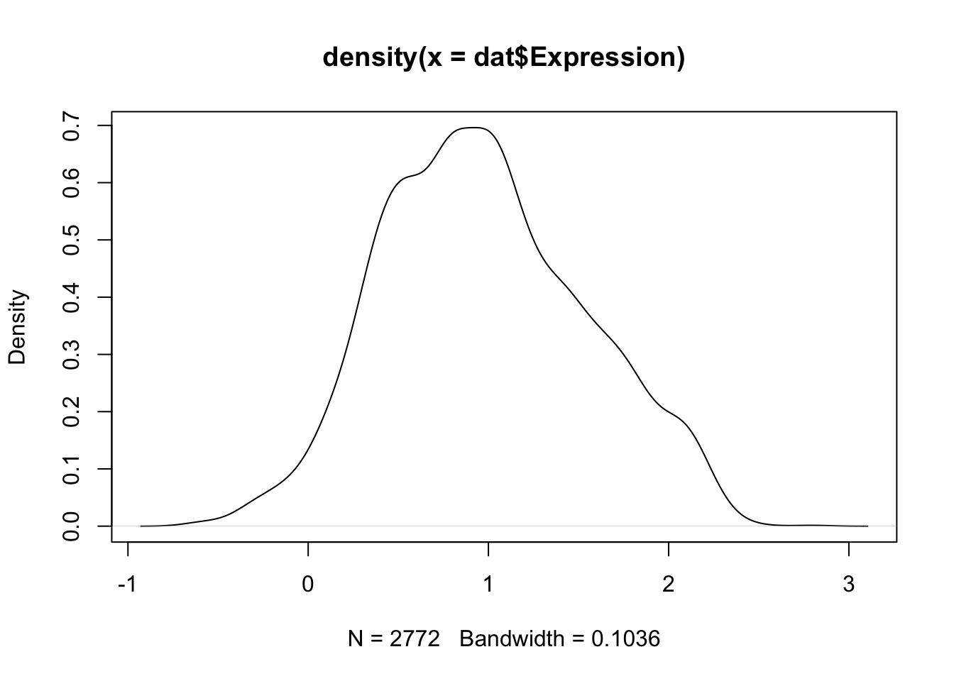
dat %>%
  dplyr::filter(ADT %in% top_markers) |>
  heatmap(
    .column = !!sym(grp),
    .row = ADT,
    .value = Expression,
    row_order = top_markers,
    scale = "none",
    rect_gp = grid::gpar(col = "white", lwd = 1),
    show_row_names = TRUE,
    cluster_columns = FALSE,
    cluster_rows = FALSE,
    column_names_gp = grid::gpar(fontsize = 10),
    column_title_gp = grid::gpar(fontsize = 12),
    row_names_gp = grid::gpar(fontsize = 8, col = cols[order(top_markers)]),
    row_title_gp = grid::gpar(fontsize = 12),
    column_title_side = "top",
    palette_value = circlize::colorRamp2(seq(-0.5, 2.5, length.out = 256),
                                         viridis::magma(256)),
    heatmap_legend_param = list(direction = "vertical"))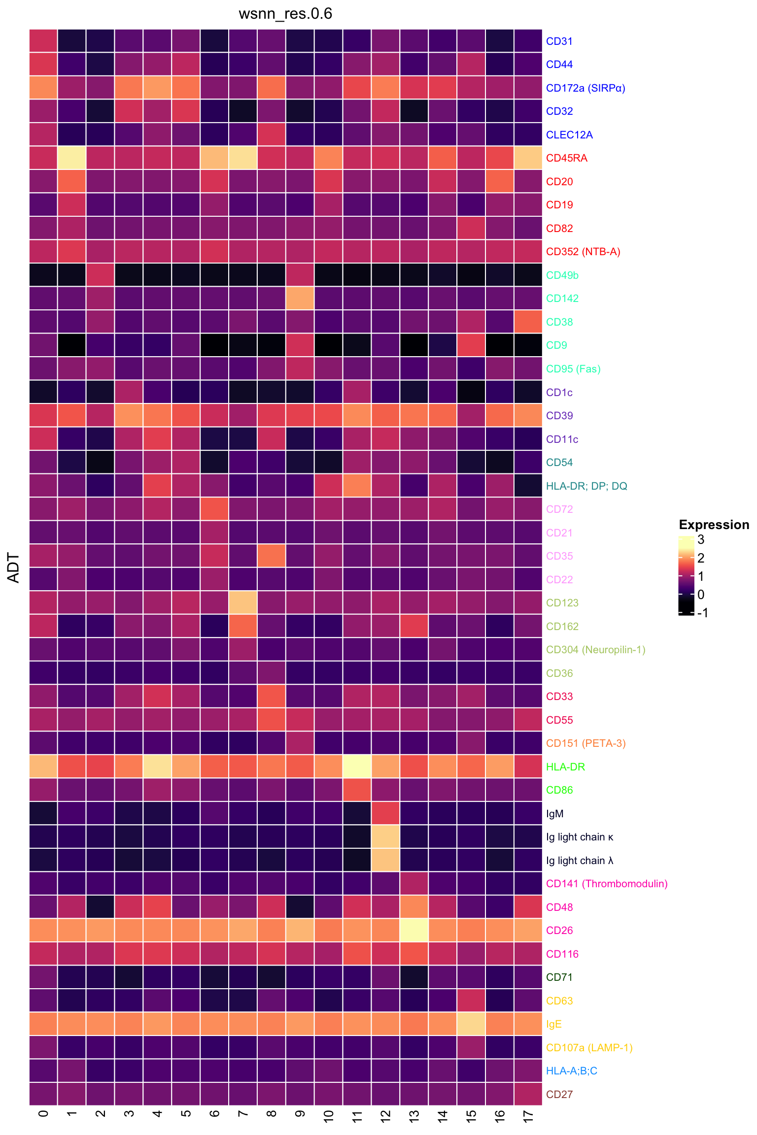
Save ADT markers
options(scipen=-1, digits = 6)
contnames <- colnames(mycont)
dirName <- here("output",
                "cluster_markers",
                glue("ADT{ambient}"),
                "other_cells")
if(!dir.exists(dirName)) dir.create(dirName, recursive = TRUE)

for(c in contnames){
  top <- topTreat(tr, coef = c, n = Inf)
  top <- top[top$logFC > 0, ]
  write.csv(top,
            file = glue("{dirName}/up-cluster-limma-{c}.csv"),
            sep = ",",
            quote = FALSE,
            col.names = NA,
            row.names = TRUE)
}
Session info
sessionInfo()R version 4.3.2 (2023-10-31)
Platform: aarch64-apple-darwin20 (64-bit)
Running under: macOS Sonoma 14.3.1
Matrix products: default
BLAS: /Library/Frameworks/R.framework/Versions/4.3-arm64/Resources/lib/libRblas.0.dylib
LAPACK: /Library/Frameworks/R.framework/Versions/4.3-arm64/Resources/lib/libRlapack.dylib; LAPACK version 3.11.0
locale:
[1] en_US.UTF-8/en_US.UTF-8/en_US.UTF-8/C/en_US.UTF-8/en_US.UTF-8
time zone: Australia/Melbourne
tzcode source: internal
attached base packages:
[1] stats4 stats graphics grDevices datasets utils methods
[8] base
other attached packages:
[1] dsb_1.0.3 tidyHeatmap_1.8.1
[3] speckle_1.2.0 glue_1.7.0
[5] org.Hs.eg.db_3.18.0 AnnotationDbi_1.64.1
[7] patchwork_1.2.0 clustree_0.5.1
[9] ggraph_2.2.0 here_1.0.1
[11] dittoSeq_1.14.2 glmGamPoi_1.14.3
[13] SeuratObject_4.1.4 Seurat_4.4.0
[15] lubridate_1.9.3 forcats_1.0.0
[17] stringr_1.5.1 dplyr_1.1.4
[19] purrr_1.0.2 readr_2.1.5
[21] tidyr_1.3.1 tibble_3.2.1
[23] ggplot2_3.5.0 tidyverse_2.0.0
[25] edgeR_4.0.15 limma_3.58.1
[27] SingleCellExperiment_1.24.0 SummarizedExperiment_1.32.0
[29] Biobase_2.62.0 GenomicRanges_1.54.1
[31] GenomeInfoDb_1.38.6 IRanges_2.36.0
[33] S4Vectors_0.40.2 BiocGenerics_0.48.1
[35] MatrixGenerics_1.14.0 matrixStats_1.2.0
[37] workflowr_1.7.1
loaded via a namespace (and not attached):
[1] fs_1.6.3 spatstat.sparse_3.0-3 bitops_1.0-7
[4] httr_1.4.7 RColorBrewer_1.1-3 doParallel_1.0.17
[7] backports_1.4.1 tools_4.3.2 sctransform_0.4.1
[10] utf8_1.2.4 R6_2.5.1 lazyeval_0.2.2
[13] uwot_0.1.16 GetoptLong_1.0.5 withr_3.0.0
[16] sp_2.1-3 gridExtra_2.3 progressr_0.14.0
[19] cli_3.6.2 Cairo_1.6-2 spatstat.explore_3.2-6
[22] prismatic_1.1.1 labeling_0.4.3 sass_0.4.8
[25] spatstat.data_3.0-4 ggridges_0.5.6 pbapply_1.7-2
[28] parallelly_1.37.0 rstudioapi_0.15.0 RSQLite_2.3.5
[31] generics_0.1.3 shape_1.4.6 vroom_1.6.5
[34] ica_1.0-3 spatstat.random_3.2-2 dendextend_1.17.1
[37] Matrix_1.6-5 ggbeeswarm_0.7.2 fansi_1.0.6
[40] abind_1.4-5 lifecycle_1.0.4 whisker_0.4.1
[43] yaml_2.3.8 SparseArray_1.2.4 Rtsne_0.17
[46] paletteer_1.6.0 grid_4.3.2 blob_1.2.4
[49] promises_1.2.1 crayon_1.5.2 miniUI_0.1.1.1
[52] lattice_0.22-5 cowplot_1.1.3 KEGGREST_1.42.0
[55] pillar_1.9.0 knitr_1.45 ComplexHeatmap_2.18.0
[58] rjson_0.2.21 future.apply_1.11.1 codetools_0.2-19
[61] leiden_0.4.3.1 getPass_0.2-4 data.table_1.15.0
[64] vctrs_0.6.5 png_0.1-8 gtable_0.3.4
[67] rematch2_2.1.2 cachem_1.0.8 xfun_0.42
[70] S4Arrays_1.2.0 mime_0.12 tidygraph_1.3.1
[73] survival_3.5-8 pheatmap_1.0.12 iterators_1.0.14
[76] statmod_1.5.0 ellipsis_0.3.2 fitdistrplus_1.1-11
[79] ROCR_1.0-11 nlme_3.1-164 bit64_4.0.5
[82] RcppAnnoy_0.0.22 rprojroot_2.0.4 bslib_0.6.1
[85] irlba_2.3.5.1 vipor_0.4.7 KernSmooth_2.23-22
[88] colorspace_2.1-0 DBI_1.2.1 ggrastr_1.0.2
[91] tidyselect_1.2.0 processx_3.8.3 bit_4.0.5
[94] compiler_4.3.2 git2r_0.33.0 DelayedArray_0.28.0
[97] plotly_4.10.4 checkmate_2.3.1 scales_1.3.0
[100] lmtest_0.9-40 callr_3.7.3 digest_0.6.34
[103] goftest_1.2-3 spatstat.utils_3.0-4 rmarkdown_2.25
[106] XVector_0.42.0 htmltools_0.5.7 pkgconfig_2.0.3
[109] highr_0.10 fastmap_1.1.1 rlang_1.1.3
[112] GlobalOptions_0.1.2 htmlwidgets_1.6.4 shiny_1.8.0
[115] farver_2.1.1 jquerylib_0.1.4 zoo_1.8-12
[118] jsonlite_1.8.8 mclust_6.1 RCurl_1.98-1.14
[121] magrittr_2.0.3 GenomeInfoDbData_1.2.11 munsell_0.5.0
[124] Rcpp_1.0.12 viridis_0.6.5 reticulate_1.35.0
[127] stringi_1.8.3 zlibbioc_1.48.0 MASS_7.3-60.0.1
[130] plyr_1.8.9 parallel_4.3.2 listenv_0.9.1
[133] ggrepel_0.9.5 deldir_2.0-2 Biostrings_2.70.2
[136] graphlayouts_1.1.0 splines_4.3.2 tensor_1.5
[139] hms_1.1.3 circlize_0.4.15 locfit_1.5-9.8
[142] ps_1.7.6 igraph_2.0.1.1 spatstat.geom_3.2-8
[145] reshape2_1.4.4 evaluate_0.23 renv_1.0.3
[148] tzdb_0.4.0 foreach_1.5.2 tweenr_2.0.3
[151] httpuv_1.6.14 RANN_2.6.1 polyclip_1.10-6
[154] future_1.33.1 clue_0.3-65 scattermore_1.2
[157] ggforce_0.4.2 xtable_1.8-4 later_1.3.2
[160] viridisLite_0.4.2 memoise_2.0.1 beeswarm_0.4.0
[163] cluster_2.1.6 timechange_0.3.0 globals_0.16.2