Last updated: 2024-08-25

Checks: 7 0

Knit directory: paed-inflammation-CITEseq/

This reproducible R Markdown analysis was created with workflowr (version 1.7.1). The Checks tab describes the reproducibility checks that were applied when the results were created. The Past versions tab lists the development history.

R Markdown file: up-to-date

Great! Since the R Markdown file has been committed to the Git repository, you know the exact version of the code that produced these results.

Environment: empty

Great job! The global environment was empty. Objects defined in the global environment can affect the analysis in your R Markdown file in unknown ways. For reproduciblity it’s best to always run the code in an empty environment.

Seed: set.seed(20240216)

The command set.seed(20240216) was run prior to running the code in the R Markdown file. Setting a seed ensures that any results that rely on randomness, e.g. subsampling or permutations, are reproducible.

Session information: recorded

Great job! Recording the operating system, R version, and package versions is critical for reproducibility.

Cache: none

Nice! There were no cached chunks for this analysis, so you can be confident that you successfully produced the results during this run.

File paths: relative

Great job! Using relative paths to the files within your workflowr project makes it easier to run your code on other machines.

Repository version: 70b3aa0

Great! You are using Git for version control. Tracking code development and connecting the code version to the results is critical for reproducibility.

The results in this page were generated with repository version 70b3aa0. See the Past versions tab to see a history of the changes made to the R Markdown and HTML files.

Note that you need to be careful to ensure that all relevant files for the analysis have been committed to Git prior to generating the results (you can use wflow_publish or wflow_git_commit). workflowr only checks the R Markdown file, but you know if there are other scripts or data files that it depends on. Below is the status of the Git repository when the results were generated:


Ignored files:
    Ignored:    .Rhistory
    Ignored:    .Rproj.user/
    Ignored:    analysis/figure/
    Ignored:    data/C133_Neeland_batch1/
    Ignored:    data/C133_Neeland_merged/
    Ignored:    renv/library/
    Ignored:    renv/staging/

Untracked files:
    Untracked:  analysis/15.0_integrate_all_cells.Rmd

Unstaged changes:
    Modified:   analysis/09.0_integrate_cluster_macro_cells.Rmd

Note that any generated files, e.g. HTML, png, CSS, etc., are not included in this status report because it is ok for generated content to have uncommitted changes.

These are the previous versions of the repository in which changes were made to the R Markdown (analysis/10.0_manual_annotations_macro_cells.Rmd) and HTML (docs/10.0_manual_annotations_macro_cells.html) files. If you’ve configured a remote Git repository (see ?wflow_git_remote), click on the hyperlinks in the table below to view the files as they were in that past version.

File	Version	Author	Date	Message
Rmd	70b3aa0	Jovana Maksimovic	2024-08-25	wflow_publish("analysis/10.0_manual_annotations_macro_cells.Rmd")
Rmd	d6f636a	Jovana Maksimovic	2024-08-25	Update manual macrophage annotations with new levels.
html	4cde7d9	Jovana Maksimovic	2024-06-28	Build site.
Rmd	ff98580	Jovana Maksimovic	2024-06-28	wflow_publish("analysis/10.0_manual_annotations_macro_cells.Rmd")
Rmd	a4db7cf	Jovana Maksimovic	2024-06-26	Update code for adding manual annotations to macrophages without ambient correction

Load libraries

Load Data

ambient <- ""
out <- here("data",
            "C133_Neeland_merged",
            glue("C133_Neeland_full_clean{ambient}_integrated_clustered_macrophages.SEU.rds"))
seuInt <- readRDS(file = out)

seuInt

An object of class Seurat 
46108 features across 165553 samples within 5 assays 
Active assay: integrated (3000 features, 2870 variable features)
 4 other assays present: RNA, ADT, ADT.dsb, SCT
 2 dimensional reductions calculated: pca, umap

Update group labels

seuInt@meta.data %>%
  data.frame %>%
  mutate(Group = ifelse(str_detect(Treatment, "ivacaftor"),
                        "CF.IVA",
                        ifelse(str_detect(Treatment, "orkambi"),
                               "CF.LUMA_IVA",
                               ifelse(Treatment == "untreated",
                                      "CF.NO_MOD",
                                      "NON_CF.CTRL"))),
         Group_severity = ifelse(!Group %in% "NON_CF.CTRL", 
                                 paste(Group, 
                                       toupper(substr(Severity, 1, 1)),
                                       sep = "."), 
                                 Group),
         Severity = tolower(Severity),
         Participant = strsplit2(sample.id, ".", fixed = TRUE)[,1]) -> seuInt@meta.data

Sub-cluster labelling

Load manual annotations

labels <- read_excel(here("data",
                          "cluster_annotations",
                          "macrophages_26.06.24.xlsx"))

# set selected cluster resolution
grp <- "integrated_snn_res.0.6"
seuInt@meta.data %>%
  rownames_to_column(var = "cell") %>%
  left_join(labels %>%
              mutate(Cluster = as.factor(Cluster),
                     ann_level_2 = as.factor(ann_level_2),
                     ann_level_1 = as.factor(ann_level_1)),
            by = c("integrated_snn_res.0.6" = "Cluster")) %>%
  column_to_rownames(var = "cell") -> seuInt@meta.data

seuInt <- subset(seuInt, cells = which(seuInt$ann_level_2 != "unknown"))
seuInt$ann_level_2 <- fct_drop(seuInt$ann_level_2)
seuInt$ann_level_1 <- fct_drop(seuInt$ann_level_1)
seuInt

An object of class Seurat 
46108 features across 165209 samples within 5 assays 
Active assay: integrated (3000 features, 2870 variable features)
 4 other assays present: RNA, ADT, ADT.dsb, SCT
 2 dimensional reductions calculated: pca, umap

Update PCA and UMAP after removing “unknown” cell clusters.

# redo PCA and UMAP 
seuInt <- RunPCA(seuInt, dims = 1:30, verbose = FALSE) %>%
  RunUMAP(dims = 1:30, verbose = FALSE)

Visualise annotations

options(ggrepel.max.overlaps = Inf)
DimPlot(seuInt, reduction = 'umap', label = TRUE, repel = TRUE, 
        label.size = 3, group.by = "integrated_snn_res.0.6") + 
  NoLegend() -> p1

cluster_pal <- "ggsci::category20_d3"
DimPlot(seuInt, reduction = 'umap', label = FALSE, group.by = "ann_level_2") + 
  scale_color_paletteer_d(cluster_pal) +
  theme(text = element_text(size = 9),
        axis.text = element_blank(),
        axis.ticks = element_blank()) +
  NoLegend() -> p2

DimPlot(seuInt, reduction = 'umap', label = FALSE, group.by = "ann_level_3") + 
  scale_color_paletteer_d(cluster_pal) +
  theme(text = element_text(size = 9),
        axis.text = element_blank(),
        axis.ticks = element_blank()) +
  NoLegend() -> p3

p1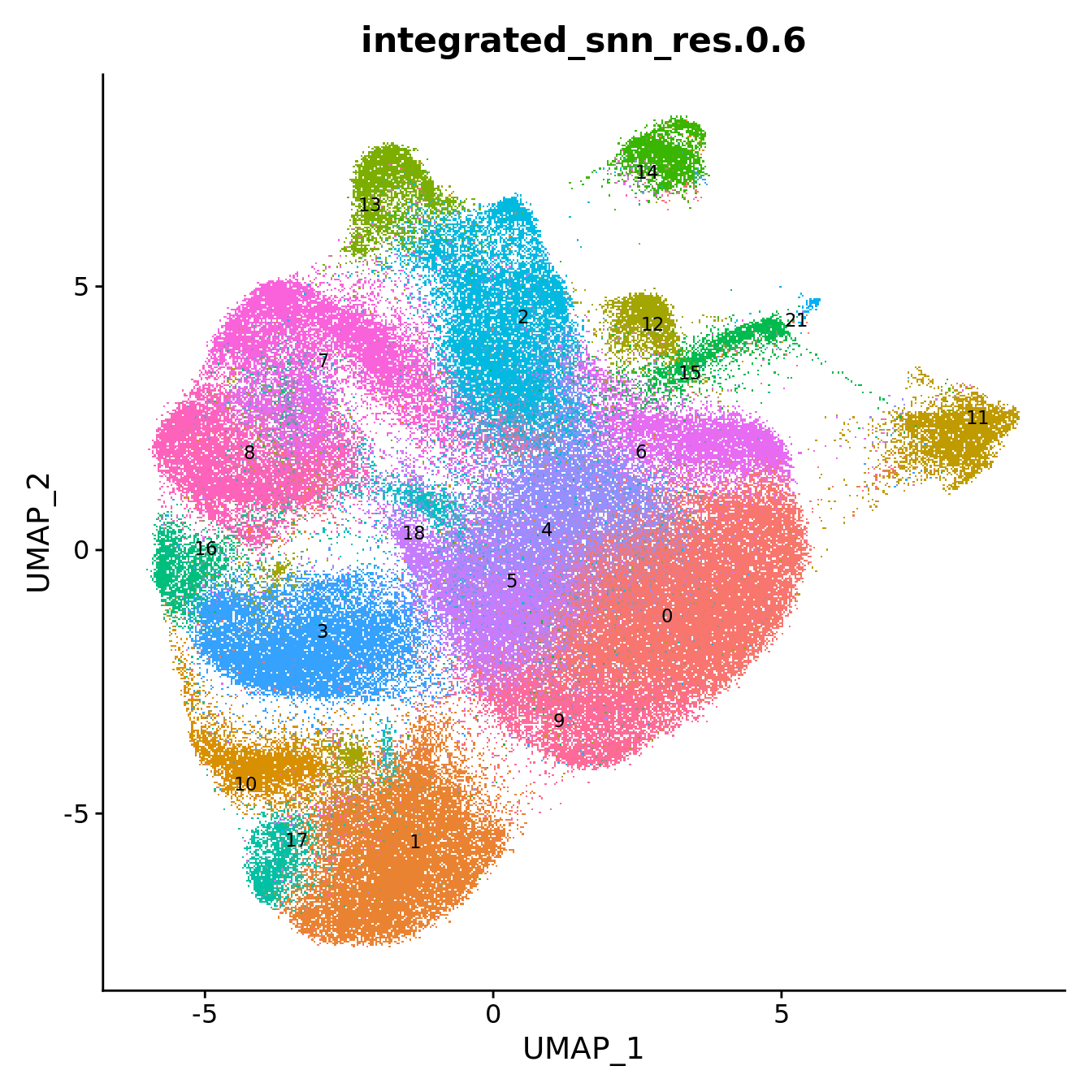

Version	Author	Date
4cde7d9	Jovana Maksimovic	2024-06-28

LabelClusters(p2, id = "ann_level_2", repel = TRUE, 
              size = 2.5, box = TRUE, fontfamily = "arial")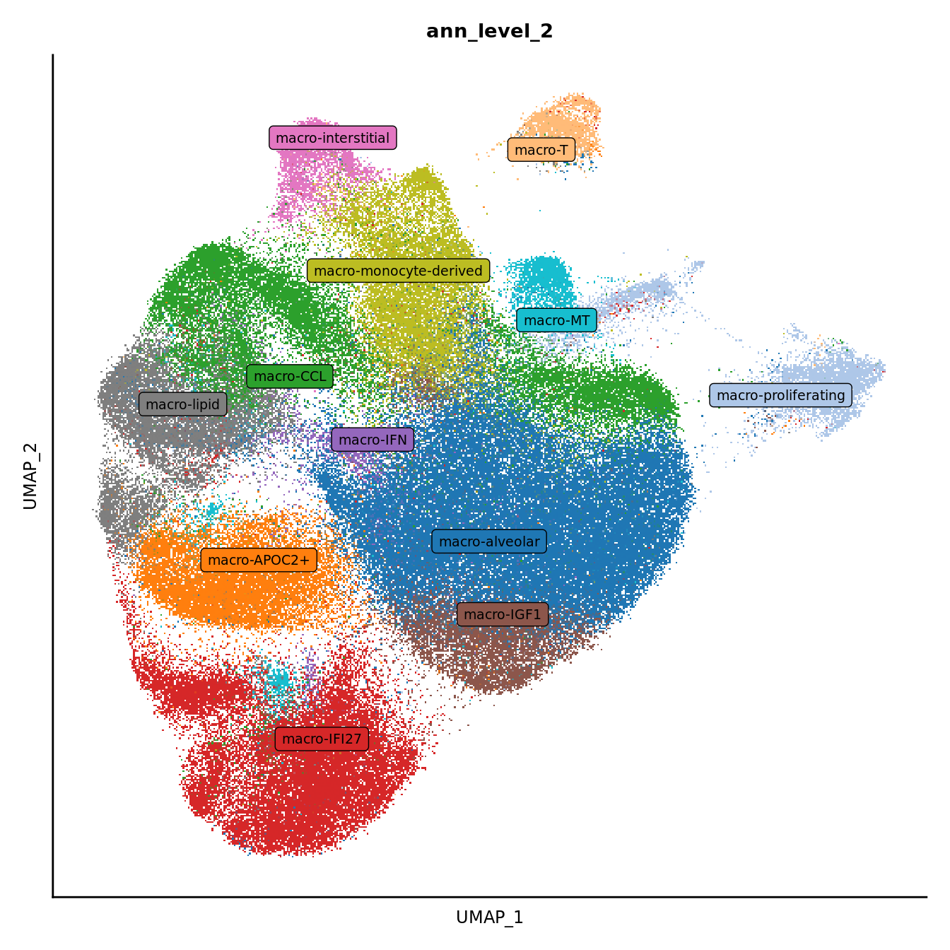

Version	Author	Date
4cde7d9	Jovana Maksimovic	2024-06-28

LabelClusters(p3, id = "ann_level_3", repel = TRUE, 
              size = 2.5, box = TRUE, fontfamily = "arial")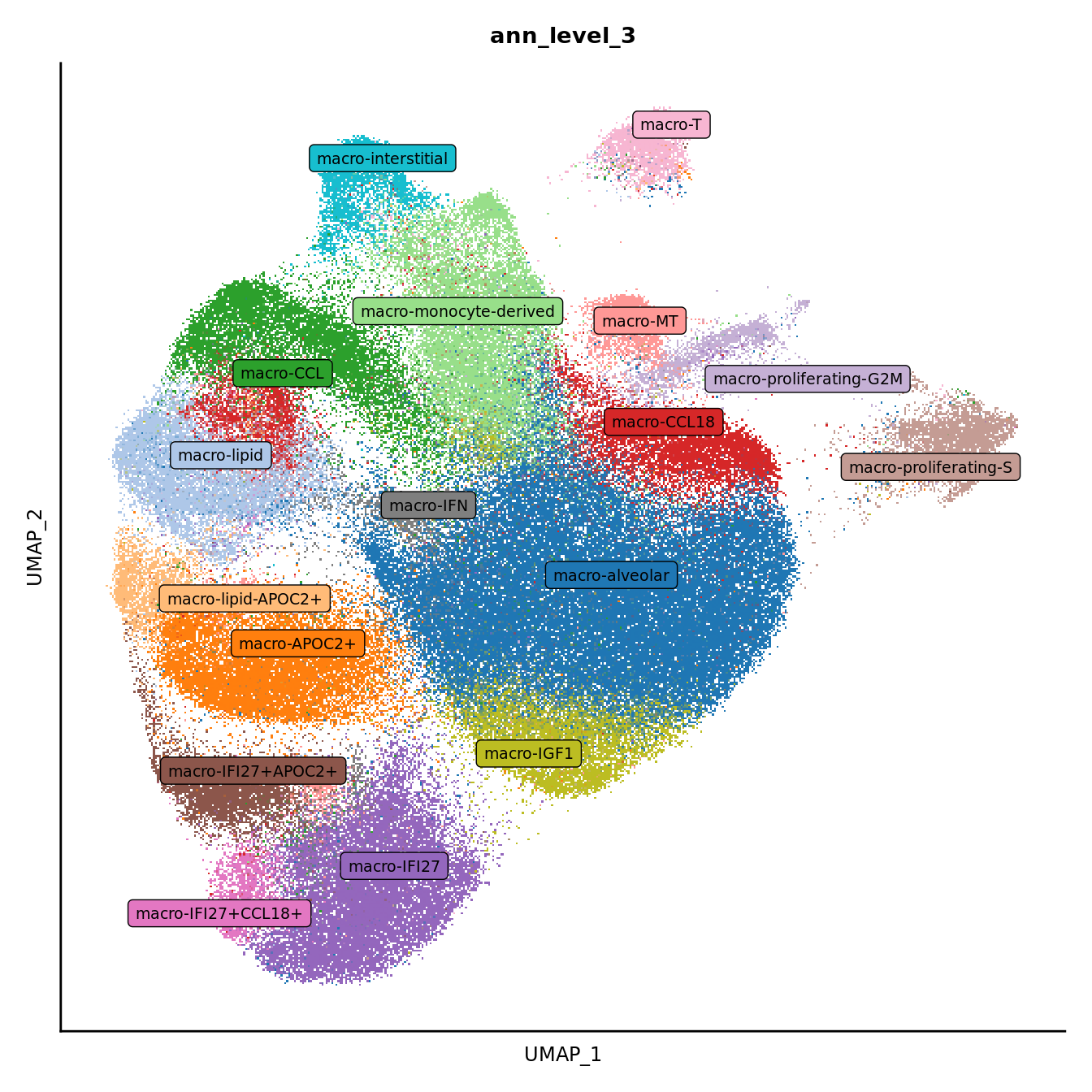

No. cells per cluster

seuInt@meta.data %>%
  ggplot(aes(x = ann_level_2, fill = ann_level_2)) +
  geom_bar() +
  geom_text(aes(label = after_stat(count)), stat = "count",
            vjust = -0.5, colour = "black", size = 2) +
  theme_classic() +
  theme(axis.text.x = element_text(angle = 90, vjust = 0.5, hjust = 1)) +
  NoLegend() +
  scale_fill_paletteer_d(cluster_pal)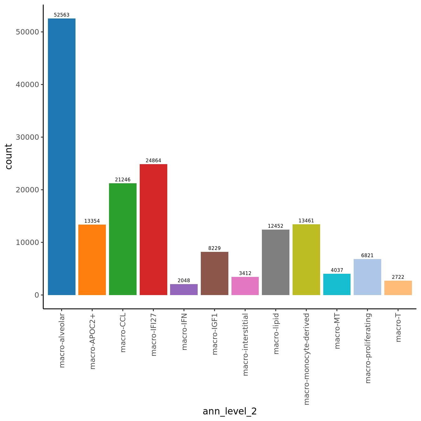

Version	Author	Date
4cde7d9	Jovana Maksimovic	2024-06-28

seuInt@meta.data %>%
  ggplot(aes(x = ann_level_3, fill = ann_level_3)) +
  geom_bar() +
  geom_text(aes(label = after_stat(count)), stat = "count",
            vjust = -0.5, colour = "black", size = 2) +
  theme_classic() +
  theme(axis.text.x = element_text(angle = 90, vjust = 0.5, hjust = 1)) +
  NoLegend() +
  scale_fill_paletteer_d(cluster_pal)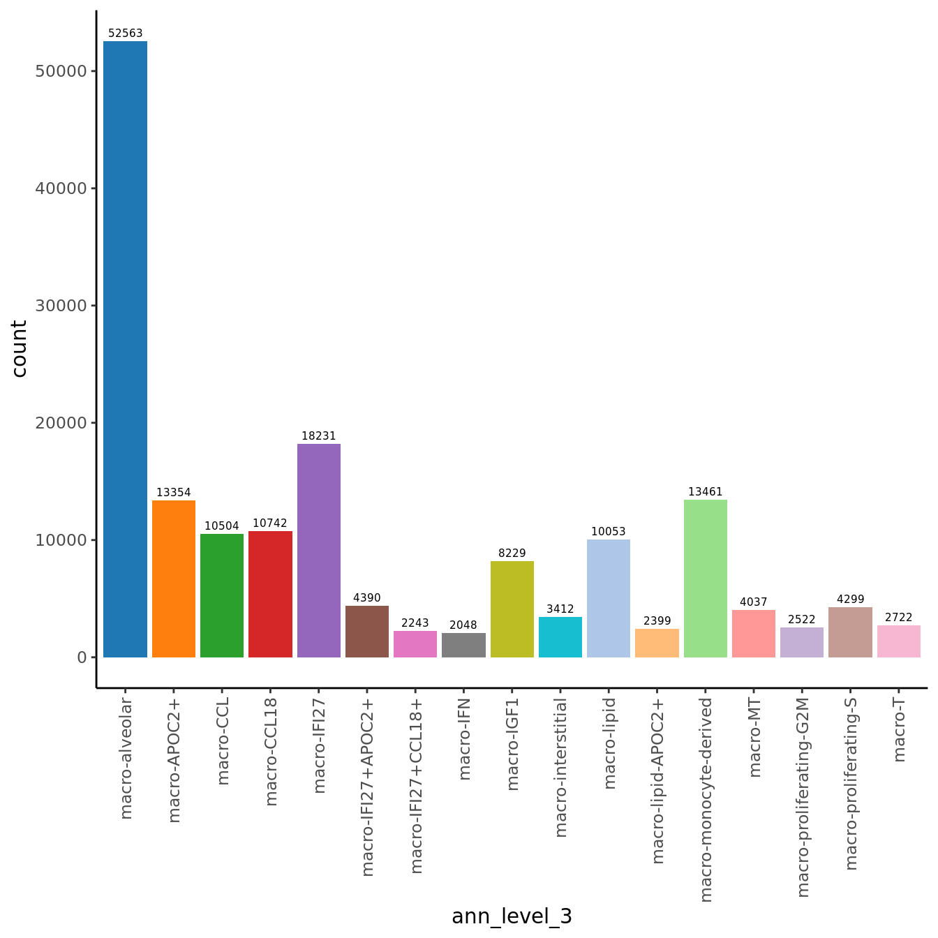

% cells per cluster

seuInt@meta.data %>% 
  count(ann_level_2) %>% 
  mutate(perc = round(n/sum(n)*100, 1)) %>%
  dplyr::rename(`Cell Label` = "ann_level_2", 
                `No. Cells` = n,
                `% Cells` = perc) %>%
  knitr::kable()

Cell Label	No. Cells	% Cells
macro-alveolar	52563	31.8
macro-APOC2+	13354	8.1
macro-CCL	21246	12.9
macro-IFI27	24864	15.1
macro-IFN	2048	1.2
macro-IGF1	8229	5.0
macro-interstitial	3412	2.1
macro-lipid	12452	7.5
macro-monocyte-derived	13461	8.1
macro-MT	4037	2.4
macro-proliferating	6821	4.1
macro-T	2722	1.6

seuInt@meta.data %>% 
  count(ann_level_3) %>% 
  mutate(perc = round(n/sum(n)*100, 1)) %>%
  dplyr::rename(`Cell Label` = "ann_level_3", 
                `No. Cells` = n,
                `% Cells` = perc) %>%
  knitr::kable()

Cell Label	No. Cells	% Cells
macro-APOC2+	13354	8.1
macro-CCL	10504	6.4
macro-CCL18	10742	6.5
macro-IFI27	18231	11.0
macro-IFI27+APOC2+	4390	2.7
macro-IFI27+CCL18+	2243	1.4
macro-IFN	2048	1.2
macro-IGF1	8229	5.0
macro-MT	4037	2.4
macro-T	2722	1.6
macro-alveolar	52563	31.8
macro-interstitial	3412	2.1
macro-lipid	10053	6.1
macro-lipid-APOC2+	2399	1.5
macro-monocyte-derived	13461	8.1
macro-proliferating-G2M	2522	1.5
macro-proliferating-S	4299	2.6

RNA marker gene analysis

Adapted from Dr. Belinda Phipson’s work for [@Sim2021-cg].

Test for marker genes using `limma`

# limma-trend for DE
Idents(seuInt) <- "ann_level_3"

out <- here("data",
            "C133_Neeland_merged",
            glue("C133_Neeland_full_clean{ambient}_macrophages_logcounts.SEU.rds"))

if(!file.exists(out)){
  logcounts <- normCounts(DGEList(as.matrix(seuInt[["RNA"]]@counts)),
                          log = TRUE, prior.count = 0.5)
  entrez <- AnnotationDbi::mapIds(org.Hs.eg.db,
                                  keys = rownames(logcounts),
                                  column = c("ENTREZID"),
                                  keytype = "SYMBOL",
                                  multiVals = "first")
  # remove genes without entrez IDs as these are difficult to interpret biologically
  logcounts <- logcounts[!is.na(entrez),]
  saveRDS(logcounts, file = out)
  
} else {
  logcounts <- readRDS(out)  
}

maxclust <- length(levels(Idents(seuInt))) - 1

clustgrp <- seuInt$ann_level_3
clustgrp <- factor(clustgrp)
donor <- factor(seuInt$sample.id)
batch <- factor(seuInt$Batch)

design <- model.matrix(~ 0 + clustgrp + donor)
colnames(design)[1:(length(levels(clustgrp)))] <- levels(clustgrp)

# Create contrast matrix
mycont <- matrix(NA, ncol = length(levels(clustgrp)),
                 nrow = length(levels(clustgrp)))
rownames(mycont) <- colnames(mycont) <- levels(clustgrp)
diag(mycont) <- 1
mycont[upper.tri(mycont)] <- -1/(length(levels(factor(clustgrp))) - 1)
mycont[lower.tri(mycont)] <- -1/(length(levels(factor(clustgrp))) - 1)

# Fill out remaining rows with 0s
zero.rows <- matrix(0, ncol = length(levels(clustgrp)),
                    nrow = (ncol(design) - length(levels(clustgrp))))
fullcont <- rbind(mycont, zero.rows)
rownames(fullcont) <- colnames(design)

fit <- lmFit(logcounts, design)

fit.cont <- contrasts.fit(fit, contrasts = fullcont)
fit.cont <- eBayes(fit.cont, trend = TRUE, robust = TRUE)

summary(decideTests(fit.cont))

       macro-alveolar macro-APOC2+ macro-CCL macro-CCL18 macro-IFI27
Down             4703         3679      4468        3261        3557
NotSig           7506         9466     10314       11349        8891
Up               4246         3310      1673        1845        4007
       macro-IFI27+APOC2+ macro-IFI27+CCL18+ macro-IFN macro-IGF1
Down                 2556               1614      1598       3086
NotSig              11569              13488     13024       9773
Up                   2330               1353      1833       3596
       macro-interstitial macro-lipid macro-lipid-APOC2+ macro-monocyte-derived
Down                 8013        7126               3911                   7999
NotSig               5657        7365              11347                   5833
Up                   2785        1964               1197                   2623
       macro-MT macro-proliferating-G2M macro-proliferating-S macro-T
Down       2505                    3464                  2193    1055
NotSig    12091                    9138                  7260   11024
Up         1859                    3853                  7002    4376

Test relative to a threshold (TREAT).

tr <- treat(fit.cont, lfc = 0.5)
dt <- decideTests(tr)
summary(dt)

       macro-alveolar macro-APOC2+ macro-CCL macro-CCL18 macro-IFI27
Down                6            3         1           2           4
NotSig          16443        16442     16420       16444       16443
Up                  6           10        34           9           8
       macro-IFI27+APOC2+ macro-IFI27+CCL18+ macro-IFN macro-IGF1
Down                    1                  1         2          9
NotSig              16443              16442     16383      16430
Up                     11                 12        70         16
       macro-interstitial macro-lipid macro-lipid-APOC2+ macro-monocyte-derived
Down                  344          35                 19                     99
NotSig              15962       16403              16416                  16325
Up                    149          17                 20                     31
       macro-MT macro-proliferating-G2M macro-proliferating-S macro-T
Down          0                      63                    12       0
NotSig    16444                   16314                 16163   16435
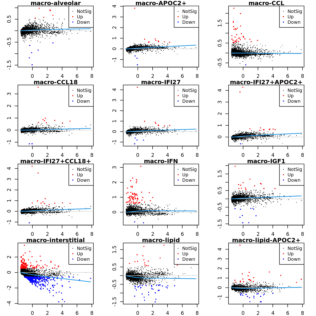
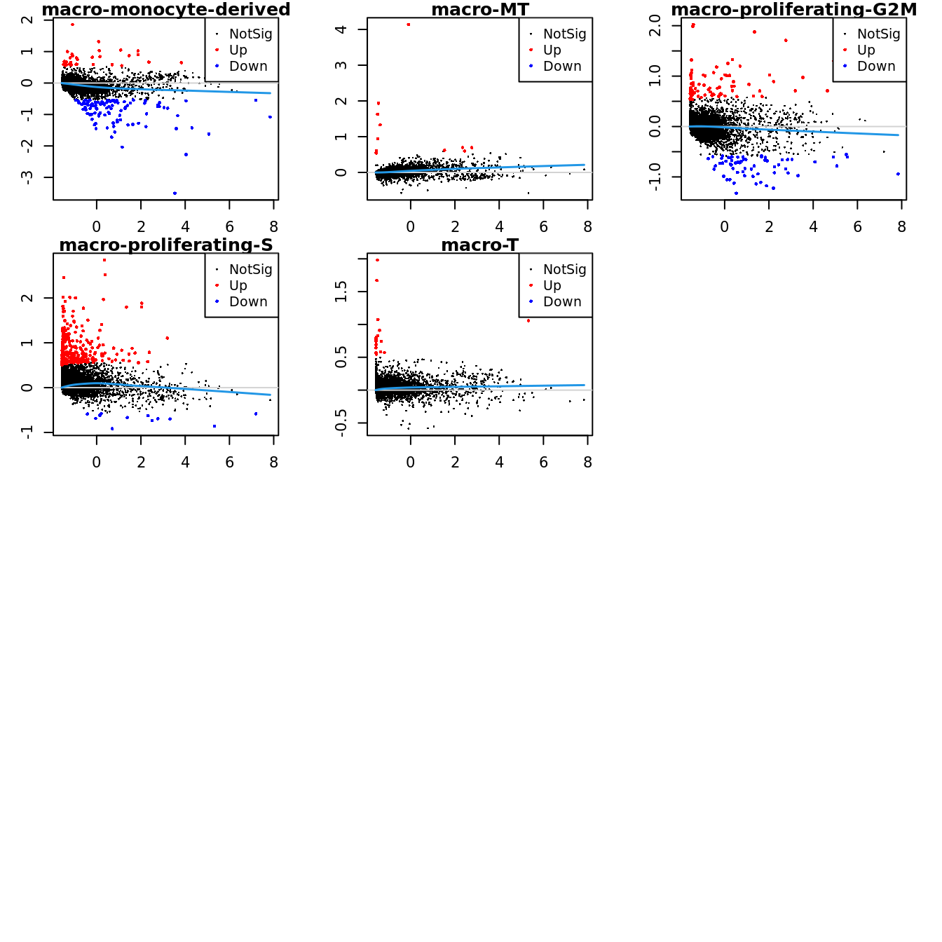
Up           11                      78                   280      20

Mean-difference (MD) plots per cluster.

par(mfrow=c(4,3))
par(mar=c(2,3,1,2))

for(i in 1:ncol(mycont)){
  plotMD(tr, coef = i, status = dt[,i], hl.cex = 0.5)
  abline(h = 0, col = "lightgrey")
  lines(lowess(tr$Amean, tr$coefficients[,i]), lwd = 1.5, col = 4)
}

`limma` marker gene dotplot

DefaultAssay(seuInt) <- "RNA"
contnames <- colnames(mycont)
top_markers <- NULL
n_markers <- 5

for(i in 1:ncol(mycont)){
  top <- topTreat(tr, coef = i, n = Inf)
  top <- top[top$logFC > 0, ]
  top_markers <- c(top_markers, 
                   setNames(rownames(top)[1:n_markers], 
                            rep(contnames[i], n_markers)))
}

top_markers <- top_markers[!is.na(top_markers)]
d <- duplicated(top_markers)
top_markers <- top_markers[!d]
geneCols <- paletteer_d(cluster_pal)[factor(names(top_markers))]

strip <- strip_themed(background_x = elem_list_rect(fill = unique(geneCols)))
DotPlot(seuInt,
        features = unname(top_markers),
        group.by = "ann_level_3",
        cols = c("azure1", "blueviolet"),
        dot.scale = 2.5,
        assay = "SCT") +
  FontSize(x.text = 9, y.text = 9) +
  labs(y = element_blank(), x = element_blank()) +
  facet_grid2(~names(top_markers), 
              scales = "free_x", 
              space = "free_x", 
              strip = strip) +
  theme(axis.text.x = element_text(angle = 90,
                                   hjust = 1,
                                   vjust = 0.5),
        legend.text = element_text(size = 8),
        legend.title = element_text(size = 9),
        strip.text = element_text(size = 0),
        text = element_text(family = "arial"),
        axis.ticks = element_blank(),
        axis.line = element_blank(),
        panel.spacing = unit(2, "mm"))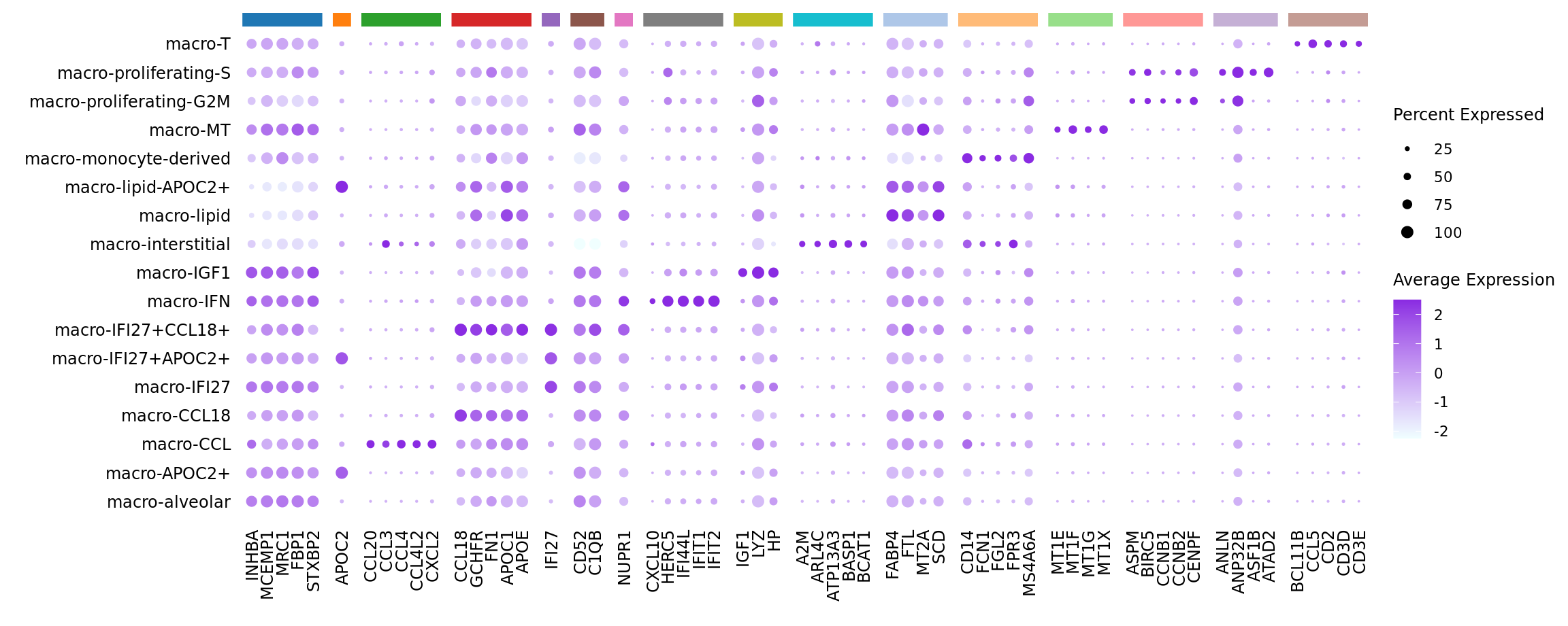

Version	Author	Date
4cde7d9	Jovana Maksimovic	2024-06-28

Test for marker genes using `Seurat`

DefaultAssay(seuInt) <- "RNA"
Idents(seuInt) <- "ann_level_3"

out <- here("data/cluster_annotations/seurat_markers_macrophages.rds")

if(!file.exists(out)){
  # restrict genes to same set as for limma analysis
  markers <- FindAllMarkers(seuInt, only.pos = TRUE, 
                            features = rownames(logcounts))
  saveRDS(markers, file = out)
  
} else {
  markers <- readRDS(out)
  
}

head(markers) %>% knitr::kable()

	avg_log2FC	pct.1	pct.2	cluster	gene
MRC1	0.3125516	0.978	0.912	macro-alveolar	MRC1
MCEMP1	0.3110134	0.979	0.893	macro-alveolar	MCEMP1
INHBA	0.3052532	0.860	0.656	macro-alveolar	INHBA
STXBP2	0.2735462	0.895	0.831	macro-alveolar	STXBP2
FBP1	0.2725335	0.978	0.943	macro-alveolar	FBP1
GPD1	0.2562846	0.572	0.425	macro-alveolar	GPD1

`Seurat` marker gene dotplot

DefaultAssay(seuInt) <- "RNA"

maxGenes <- 5
markers %>%
  group_by(cluster) %>%
  top_n(n = maxGenes, wt = avg_log2FC) -> top5

sig <- top5$gene
d <- duplicated(sig)
geneCols <- paletteer_d(cluster_pal)[top5$cluster][!d]

strip <- strip_themed(background_x = elem_list_rect(fill = unique(geneCols)))
DotPlot(seuInt,
        features = sig[!d],
        group.by = "ann_level_3",
        cols = c("azure1", "blueviolet"),
        dot.scale = 2.5,
        assay = "SCT") +
  FontSize(x.text = 9, y.text = 9) +
  labs(y = element_blank(), x = element_blank()) +
  facet_grid2(~top5$cluster[!d], 
              scales = "free_x", 
              space = "free_x", 
              strip = strip) +
  theme(axis.text.x = element_text(angle = 90,
                                   hjust = 1,
                                   vjust = 0.5),
        legend.text = element_text(size = 8),
        legend.title = element_text(size = 9),
        strip.text = element_text(size = 0),
        text = element_text(family = "arial"),
        axis.ticks = element_blank(),
        axis.line = element_blank(),
        panel.spacing = unit(2, "mm"))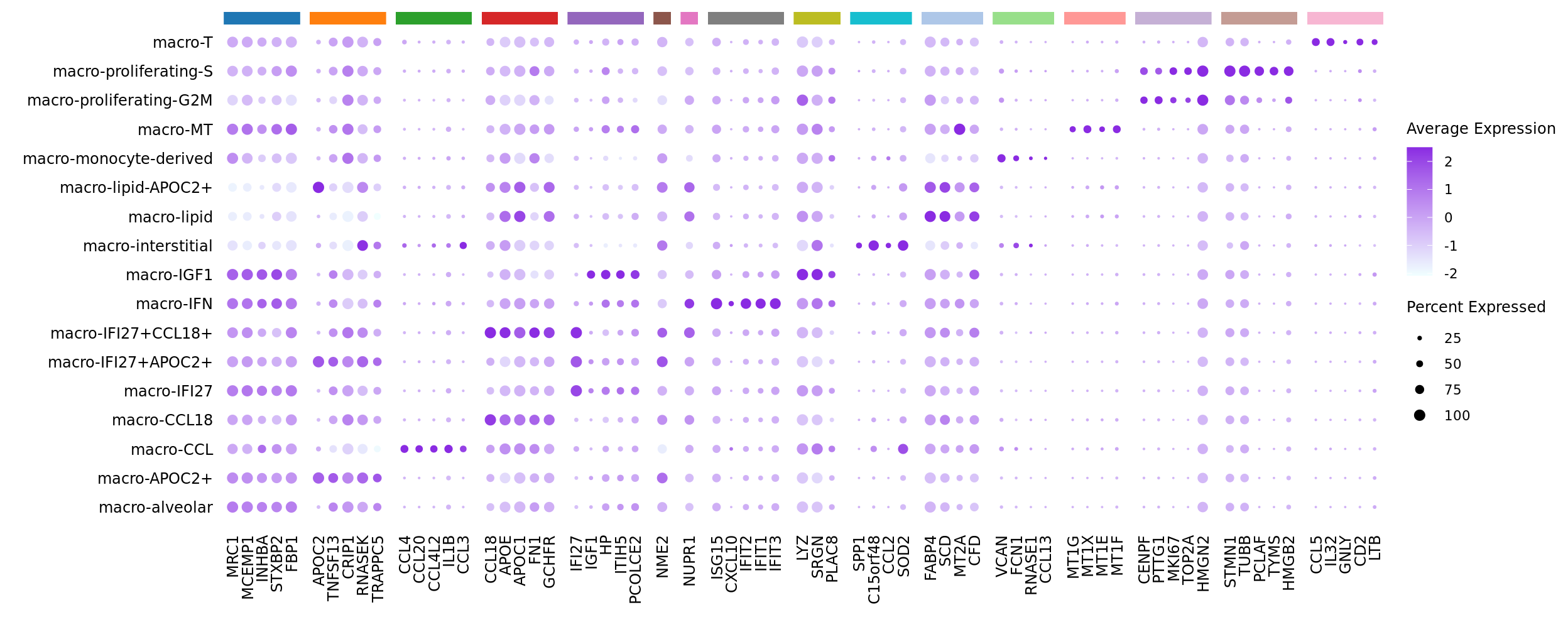

FeaturePlot(seuInt, reduction = 'umap', label = TRUE, 
            feature = "APOC2",
            label.size = 2.5,
            repel = TRUE,
            max.cutoff = 150) -> p1

FeaturePlot(seuInt, reduction = 'umap', label = TRUE, 
            feature = "IFI27",
            label.size = 2.5,
            repel = TRUE,
            max.cutoff = 150) -> p2

(p1 / p2) + 
  theme(legend.text = element_text(size = 9),
        axis.text = element_blank(),
        axis.ticks = element_blank())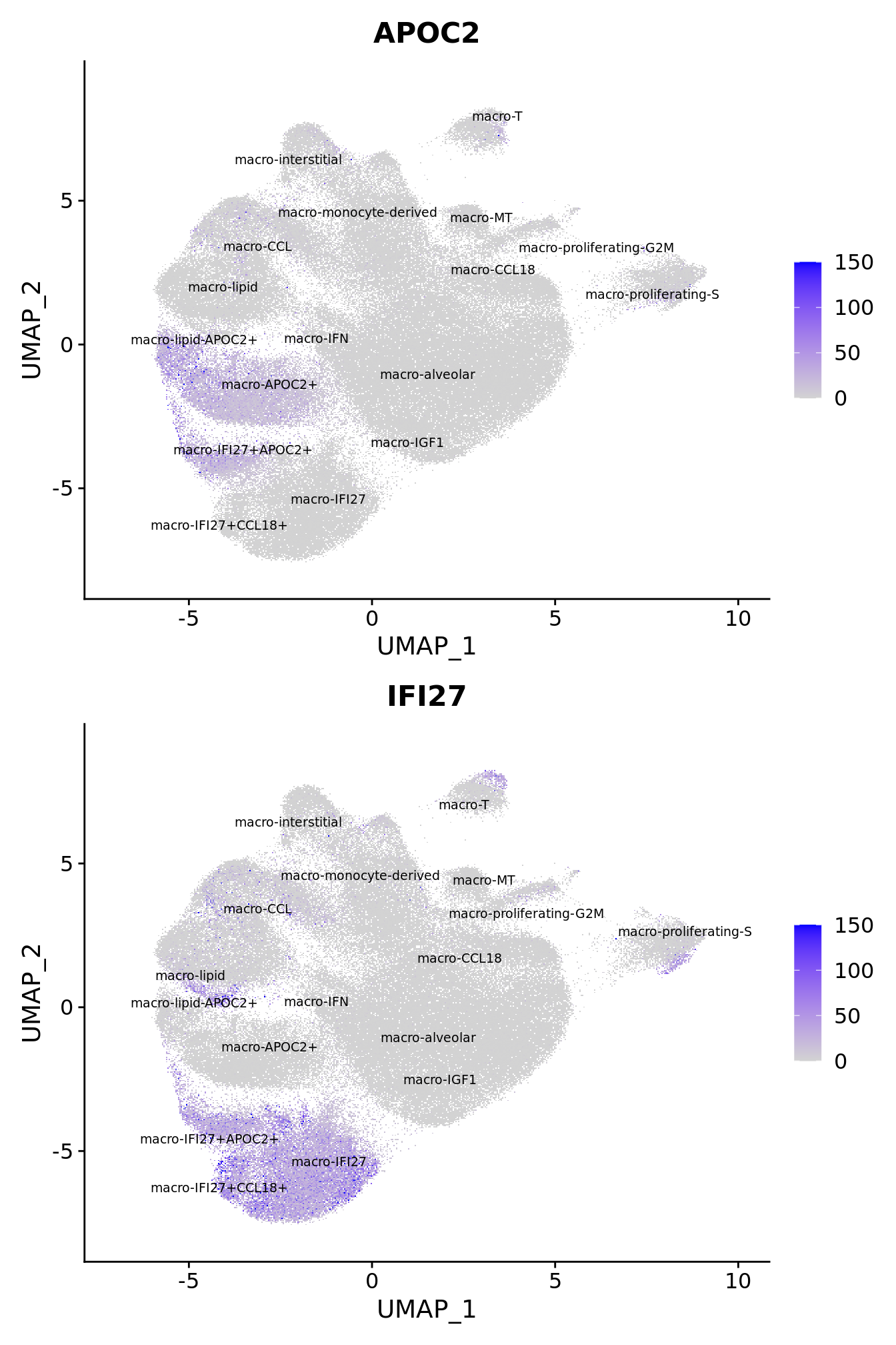

Version	Author	Date
4cde7d9	Jovana Maksimovic	2024-06-28

Visualise ADTs

Make data frame of proteins, clusters, expression levels.

out <- here("data",
            "C133_Neeland_merged",
            glue("C133_Neeland_full_clean{ambient}_macrophages_adt_dsb.rds"))

if(!file.exists(out)){
  read_csv(file = here("data",
                       "C133_Neeland_batch1",
                       "data",
                       "sample_sheets",
                       "ADT_features.csv")) -> adt_data
  
  pattern <- "anti-human/mouse |anti-human/mouse/rat |anti-mouse/human "
  adt_data$name <- gsub(pattern, "", adt_data$name)
  adt <- seuInt[["ADT"]]@counts
  if(all(rownames(seuInt[["ADT"]]@counts) == adt_data$id)) rownames(adt) <- adt_data$name
  adt_data %>%
  dplyr::filter(grepl("[Ii]sotype", name)) %>%
  pull(name) -> isotype_controls
  
  # normalise ADT using DSB normalisation
  adt_dsb <- ModelNegativeADTnorm(cell_protein_matrix = adt,
                                  denoise.counts = TRUE,
                                  use.isotype.control = TRUE,
                                  isotype.control.name.vec = isotype_controls)
  saveRDS(adt_dsb, file = out)
  
} else {
  adt_dsb <- readRDS(out)
  
}

seuInt[["ADT.dsb"]] <- NULL
m <- match(colnames(seuInt), colnames(adt_dsb)) # remove cells not present in Seurat obj
seuInt[["ADT.dsb"]] <- CreateAssayObject(data = adt_dsb[,m])

ADTs <- str_replace_all(labels$`Relevant marker ADTs`, "HLA", "HLA-")
ADTs <- ADTs[!is.na(ADTs)]
ADTs <- as.vector(t(strsplit2(str_remove_all(ADTs, " "), ",")))
ADTs <- unique(ADTs[ADTs != ""])
  
DotPlot(seuInt,
        features = ADTs,
        group.by = "ann_level_3",
        cols = c("azure1", "blueviolet"),
        dot.scale = 2.5,
        assay = "ADT.dsb") +
  FontSize(x.text = 9, y.text = 9) +
  labs(y = element_blank(), x = element_blank()) +
  theme(axis.text.x = element_text(angle = 90,
                                   hjust = 1,
                                   vjust = 0.5),
        legend.text = element_text(size = 8),
        legend.title = element_text(size = 9),
        strip.text = element_text(size = 0),
        text = element_text(family = "arial"),
        axis.ticks = element_blank(),
        axis.line = element_blank(),
        panel.spacing = unit(2, "mm"))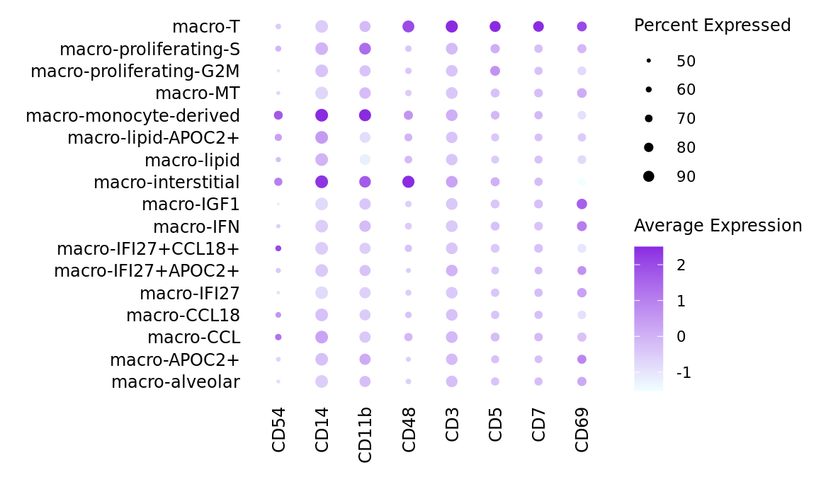

Save data

out <- here("data",
            "C133_Neeland_merged",
            glue("C133_Neeland_full_clean{ambient}_macrophages_annotated_diet.SEU.rds"))
if(!file.exists(out)){
  DefaultAssay(seuInt) <- "RNA"
  saveRDS(DietSeurat(seuInt, assays = "RNA"), out)
}

out <- here("data",
            "C133_Neeland_merged",
            glue("C133_Neeland_full_clean{ambient}_macrophages_annotated_full.SEU.rds"))
if(!file.exists(out)){
  DefaultAssay(seuInt) <- "RNA"
  saveRDS(seuInt, out)
}

Session info

sessionInfo()

R version 4.3.3 (2024-02-29)
Platform: x86_64-pc-linux-gnu (64-bit)
Running under: Ubuntu 22.04.4 LTS

Matrix products: default
BLAS:   /usr/lib/x86_64-linux-gnu/openblas-pthread/libblas.so.3 
LAPACK: /usr/lib/x86_64-linux-gnu/openblas-pthread/libopenblasp-r0.3.20.so;  LAPACK version 3.10.0

locale:
 [1] LC_CTYPE=en_AU.UTF-8       LC_NUMERIC=C              
 [3] LC_TIME=en_AU.UTF-8        LC_COLLATE=en_AU.UTF-8    
 [5] LC_MONETARY=en_AU.UTF-8    LC_MESSAGES=en_AU.UTF-8   
 [7] LC_PAPER=en_AU.UTF-8       LC_NAME=C                 
 [9] LC_ADDRESS=C               LC_TELEPHONE=C            
[11] LC_MEASUREMENT=en_AU.UTF-8 LC_IDENTIFICATION=C       

time zone: Etc/UTC
tzcode source: system (glibc)

attached base packages:
[1] stats4    stats     graphics  grDevices datasets  utils     methods  
[8] base     

other attached packages:
 [1] dsb_1.0.3                   ggh4x_0.2.8                
 [3] speckle_1.2.0               org.Hs.eg.db_3.18.0        
 [5] AnnotationDbi_1.64.1        readxl_1.4.3               
 [7] tidyHeatmap_1.8.1           paletteer_1.6.0            
 [9] patchwork_1.2.0             glue_1.7.0                 
[11] here_1.0.1                  dittoSeq_1.14.2            
[13] SeuratObject_4.1.4          Seurat_4.4.0               
[15] lubridate_1.9.3             forcats_1.0.0              
[17] stringr_1.5.1               dplyr_1.1.4                
[19] purrr_1.0.2                 readr_2.1.5                
[21] tidyr_1.3.1                 tibble_3.2.1               
[23] ggplot2_3.5.0               tidyverse_2.0.0            
[25] edgeR_4.0.15                limma_3.58.1               
[27] SingleCellExperiment_1.24.0 SummarizedExperiment_1.32.0
[29] Biobase_2.62.0              GenomicRanges_1.54.1       
[31] GenomeInfoDb_1.38.6         IRanges_2.36.0             
[33] S4Vectors_0.40.2            BiocGenerics_0.48.1        
[35] MatrixGenerics_1.14.0       matrixStats_1.2.0          
[37] workflowr_1.7.1            

loaded via a namespace (and not attached):
  [1] RcppAnnoy_0.0.22        splines_4.3.3           later_1.3.2            
  [4] prismatic_1.1.1         bitops_1.0-7            cellranger_1.1.0       
  [7] polyclip_1.10-6         lifecycle_1.0.4         doParallel_1.0.17      
 [10] rprojroot_2.0.4         globals_0.16.2          processx_3.8.3         
 [13] lattice_0.22-5          MASS_7.3-60.0.1         dendextend_1.17.1      
 [16] magrittr_2.0.3          plotly_4.10.4           sass_0.4.8             
 [19] rmarkdown_2.25          jquerylib_0.1.4         yaml_2.3.8             
 [22] httpuv_1.6.14           sctransform_0.4.1       sp_2.1-3               
 [25] spatstat.sparse_3.0-3   reticulate_1.35.0       DBI_1.2.1              
 [28] cowplot_1.1.3           pbapply_1.7-2           RColorBrewer_1.1-3     
 [31] abind_1.4-5             zlibbioc_1.48.0         Rtsne_0.17             
 [34] RCurl_1.98-1.14         git2r_0.33.0            circlize_0.4.15        
 [37] GenomeInfoDbData_1.2.11 ggrepel_0.9.5           irlba_2.3.5.1          
 [40] listenv_0.9.1           spatstat.utils_3.0-4    pheatmap_1.0.12        
 [43] goftest_1.2-3           spatstat.random_3.2-2   fitdistrplus_1.1-11    
 [46] parallelly_1.37.0       leiden_0.4.3.1          codetools_0.2-19       
 [49] DelayedArray_0.28.0     shape_1.4.6             tidyselect_1.2.0       
 [52] farver_2.1.1            viridis_0.6.5           spatstat.explore_3.2-6 
 [55] jsonlite_1.8.8          GetoptLong_1.0.5        ellipsis_0.3.2         
 [58] progressr_0.14.0        iterators_1.0.14        ggridges_0.5.6         
 [61] survival_3.7-0          foreach_1.5.2           tools_4.3.3            
 [64] ica_1.0-3               Rcpp_1.0.12             gridExtra_2.3          
 [67] SparseArray_1.2.4       xfun_0.42               withr_3.0.0            
 [70] BiocManager_1.30.22     fastmap_1.1.1           fansi_1.0.6            
 [73] callr_3.7.3             digest_0.6.34           timechange_0.3.0       
 [76] R6_2.5.1                mime_0.12               colorspace_2.1-0       
 [79] scattermore_1.2         tensor_1.5              RSQLite_2.3.5          
 [82] spatstat.data_3.0-4     utf8_1.2.4              generics_0.1.3         
 [85] renv_1.0.3              data.table_1.15.0       httr_1.4.7             
 [88] htmlwidgets_1.6.4       S4Arrays_1.2.0          whisker_0.4.1          
 [91] uwot_0.1.16             pkgconfig_2.0.3         gtable_0.3.4           
 [94] blob_1.2.4              ComplexHeatmap_2.18.0   lmtest_0.9-40          
 [97] XVector_0.42.0          htmltools_0.5.7         clue_0.3-65            
[100] scales_1.3.0            png_0.1-8               knitr_1.45             
[103] rstudioapi_0.15.0       rjson_0.2.21            tzdb_0.4.0             
[106] reshape2_1.4.4          nlme_3.1-164            GlobalOptions_0.1.2    
[109] cachem_1.0.8            zoo_1.8-12              KernSmooth_2.23-24     
[112] parallel_4.3.3          miniUI_0.1.1.1          pillar_1.9.0           
[115] grid_4.3.3              vctrs_0.6.5             RANN_2.6.1             
[118] promises_1.2.1          xtable_1.8-4            cluster_2.1.6          
[121] evaluate_0.23           cli_3.6.2               locfit_1.5-9.8         
[124] compiler_4.3.3          rlang_1.1.3             crayon_1.5.2           
[127] future.apply_1.11.1     labeling_0.4.3          mclust_6.1             
[130] rematch2_2.1.2          ps_1.7.6                getPass_0.2-4          
[133] plyr_1.8.9              fs_1.6.3                stringi_1.8.3          
[136] viridisLite_0.4.2       deldir_2.0-2            Biostrings_2.70.2      
[139] munsell_0.5.0           lazyeval_0.2.2          spatstat.geom_3.2-8    
[142] Matrix_1.6-5            hms_1.1.3               bit64_4.0.5            
[145] future_1.33.1           KEGGREST_1.42.0         statmod_1.5.0          
[148] shiny_1.8.0             highr_0.10              ROCR_1.0-11            
[151] memoise_2.0.1           igraph_2.0.1.1          bslib_0.6.1            
[154] bit_4.0.5

Annotate Macrophage clusters

Jovana Maksimovic

August 25, 2024

Load libraries

Load Data

Update group labels

Sub-cluster labelling

Load manual annotations

Visualise annotations

No. cells per cluster

% cells per cluster

RNA marker gene analysis

Test for marker genes using `limma`

`limma` marker gene dotplot

Test for marker genes using `Seurat`

`Seurat` marker gene dotplot

Visualise ADTs

Save data

Session info

Annotate Macrophage clusters

Jovana Maksimovic

August 25, 2024

Load libraries

Load Data

Update group labels

Sub-cluster labelling

Load manual annotations

Visualise annotations

No. cells per cluster

% cells per cluster

RNA marker gene analysis

Test for marker genes using limma

limma marker gene dotplot

Test for marker genes using Seurat

Seurat marker gene dotplot

Visualise ADTs

Save data

Session info

Test for marker genes using `limma`

`limma` marker gene dotplot

Test for marker genes using `Seurat`

`Seurat` marker gene dotplot