barbieQ_paper_Figure3_FigureS3: Type I error rate and power using Mixture data

workflowr

• Summary
• Checks
• Past versions

Last updated: 2026-01-11

Checks: 5 2

Knit directory: public_barcode_count/

This reproducible R Markdown analysis was created with workflowr (version 1.7.2). The Checks tab describes the reproducibility checks that were applied when the results were created. The Past versions tab lists the development history.

---

R Markdown file: uncommitted changes

The R Markdown file has unstaged changes. To know which version of the R Markdown file created these results, you’ll want to first commit it to the Git repo. If you’re still working on the analysis, you can ignore this warning. When you’re finished, you can run wflow_publish to commit the R Markdown file and build the HTML.

Environment: objects present

The global environment had objects present when the code in the R Markdown file was run. These objects can affect the analysis in your R Markdown file in unknown ways. For reproduciblity it’s best to always run the code in an empty environment. Use wflow_publish or wflow_build to ensure that the code is always run in an empty environment.

The following objects were defined in the global environment when these results were created:

Name	Class	Size
module	function	5.6 Kb

Seed: set.seed(20250112)

The command set.seed(20250112) was run prior to running the code in the R Markdown file. Setting a seed ensures that any results that rely on randomness, e.g. subsampling or permutations, are reproducible.

Session information: recorded

Great job! Recording the operating system, R version, and package versions is critical for reproducibility.

Cache: none

Nice! There were no cached chunks for this analysis, so you can be confident that you successfully produced the results during this run.

File paths: relative

Great job! Using relative paths to the files within your workflowr project makes it easier to run your code on other machines.

Repository version: ecc9192

Great! You are using Git for version control. Tracking code development and connecting the code version to the results is critical for reproducibility.

The results in this page were generated with repository version ecc9192. See the Past versions tab to see a history of the changes made to the R Markdown and HTML files.

Note that you need to be careful to ensure that all relevant files for the analysis have been committed to Git prior to generating the results (you can use wflow_publish or wflow_git_commit). workflowr only checks the R Markdown file, but you know if there are other scripts or data files that it depends on. Below is the status of the Git repository when the results were generated:

Ignored files:
    Ignored:    .RData
    Ignored:    .Rhistory
    Ignored:    .Rproj.user/
    Ignored:    public_barcode_count.Rproj

Unstaged changes:
    Modified:   analysis/barbieQ_paper_Figure3.Rmd
    Modified:   output/f3.png

Note that any generated files, e.g. HTML, png, CSS, etc., are not included in this status report because it is ok for generated content to have uncommitted changes.

---

These are the previous versions of the repository in which changes were made to the R Markdown (analysis/barbieQ_paper_Figure3.Rmd) and HTML (docs/barbieQ_paper_Figure3.html) files. If you’ve configured a remote Git repository (see ?wflow_git_remote), click on the hyperlinks in the table below to view the files as they were in that past version.

File	Version	Author	Date	Message
Rmd	670258c	FeiLiyang	2026-01-07	minor change
Rmd	f48add2	FeiLiyang	2026-01-07	supple analyses
Rmd	34f5894	FeiLiyang	2026-01-01	reorder f3
html	34f5894	FeiLiyang	2026-01-01	reorder f3
html	a2e7a36	FeiLiyang	2025-12-17	fix yml
Rmd	7b7813d	FeiLiyang	2025-12-17	update f3 fs4
html	7b7813d	FeiLiyang	2025-12-17	update f3 fs4
Rmd	c2766f9	Liyang Fei	2025-10-07	remake figures

---

1 Load Dependencies

library(readxl)
library(magrittr)
library(dplyr)
library(tidyr) # for pivot_longer
library(tibble) # for rownames_to _column
library(knitr) # for kable()
library(data.table) # for data.table()
library(SummarizedExperiment)
library(S4Vectors)
library(grid)
library(ggplot2)
library(ggbreak)
library(ggnewscale) # ggnewscale::new_scale_fill() 
library(patchwork)
library(scales)
library(ggVennDiagram)
library(ComplexHeatmap)
library(magick) # image_read()
library(eulerr)
library(edgeR)

source("analysis/plotBarcodeHistogram.R") ## accommodated from bartools::plotBarcodehistogram
source("analysis/F3_simulation.R") ## for negative simulation
source("analysis/ggplot_theme.R") ## setting ggplot theme

2 Install barbieQ

Installing the latest devel version of barbieQ from GitHub.

if (!requireNamespace("barbieQ", quietly = TRUE)) {
  remotes::install_github("Oshlack/barbieQ")
}

Warning: replacing previous import 'data.table::first' by 'dplyr::first' when
loading 'barbieQ'

Warning: replacing previous import 'data.table::last' by 'dplyr::last' when
loading 'barbieQ'

Warning: replacing previous import 'data.table::between' by 'dplyr::between'
when loading 'barbieQ'

Warning: replacing previous import 'dplyr::as_data_frame' by
'igraph::as_data_frame' when loading 'barbieQ'

Warning: replacing previous import 'dplyr::groups' by 'igraph::groups' when
loading 'barbieQ'

Warning: replacing previous import 'dplyr::union' by 'igraph::union' when
loading 'barbieQ'

library(barbieQ)

Check the version of barbieQ.

packageVersion("barbieQ")

[1] '1.1.3'

3 Set seeds

set.seed(2025)

4 Load data

load("output/mixture_barbieQ.rda")

5 F3A: Experimental schematic

schematic <- image_read("output/f3a_schematic.png")
f3a <- rasterGrob(schematic, interpolate = FALSE) 
wrap_elements(full = f3a)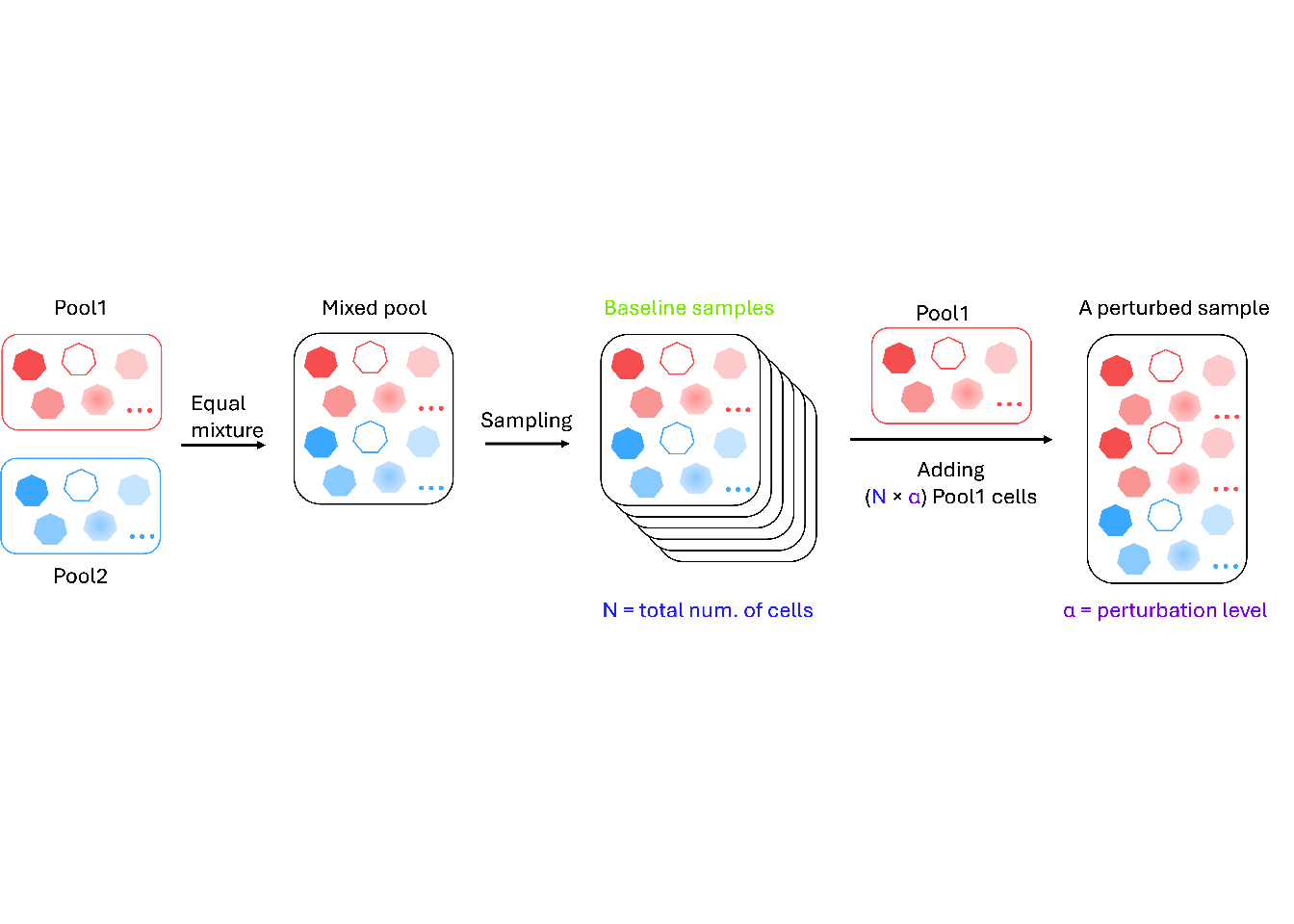

Past versions of unnamed-chunk-4-1.png

Version	Author	Date
dfa737a	FeiLiyang	2025-12-17

6 F3B: Plot barcode proportion and sample annotation

plotBarcodeHistogram, sourced from “plotBarcodeHistogram.R”, is customized from the bartools package.

## pull out sample designs
design_mixed <- mixture_plus1_top$sampleMetadata %>% as.data.frame()
design_mixed$sample <- colnames(mixture_plus1_top)
str(design_mixed)

'data.frame':   38 obs. of  5 variables:
 $ Subset      : Factor w/ 4 levels "premix1","premix2",..: 1 2 3 3 3 3 3 3 3 3 ...
 $ BarcodeSize : num  NA NA 660000 660000 330000 330000 160000 160000 80000 80000 ...
 $ Perturbation: num  NA NA 0 0 0 0 0 0 0 0 ...
 $ TechRep     : Factor w/ 2 levels "1","2": 1 1 1 2 1 2 1 2 1 2 ...
 $ sample      : chr  "P1" "P2" "null_660.1" "null_660.2" ...

design_mixed$y = 1.05
color_mapping <- mixture_plus1_top@metadata$factorColors

## order samples
order_sample <- design_mixed %>% with(order(Subset, Perturbation, BarcodeSize))

mixed_dge <- DGEList(
  counts = assay(mixture_plus1_top), 
  group = mixture_plus1_top$sampleMetadata$Subset)

## pull out ggplot data
p_mixed <- plotBarcodeHistogram(mixed_dge, orderSamples = colnames(mixture_plus1_top)[order_sample])

Warning: Use of .data in tidyselect expressions was deprecated in tidyselect 1.2.0.
ℹ Please use `"barcode"` instead of `.data$barcode`
This warning is displayed once every 8 hours.
Call `lifecycle::last_lifecycle_warnings()` to see where this warning was
generated.

Warning: Use of .data in tidyselect expressions was deprecated in tidyselect 1.2.0.
ℹ Please use `"value"` instead of `.data$value`
This warning is displayed once every 8 hours.
Call `lifecycle::last_lifecycle_warnings()` to see where this warning was
generated.

Warning: Use of .data in tidyselect expressions was deprecated in tidyselect 1.2.0.
ℹ Please use `"name"` instead of `.data$name`
This warning is displayed once every 8 hours.
Call `lifecycle::last_lifecycle_warnings()` to see where this warning was
generated.

Warning: Use of .data in tidyselect expressions was deprecated in tidyselect 1.2.0.
ℹ Please use `"freq"` instead of `.data$freq`
This warning is displayed once every 8 hours.
Call `lifecycle::last_lifecycle_warnings()` to see where this warning was
generated.

p_mixed_illus <- p_mixed +
  ## label subset
  ggnewscale::new_scale_fill() +
  geom_tile(data = design_mixed, aes(x = sample,y = y, fill = Subset), height = 0.04, inherit.aes = FALSE, color = "white") +
  scale_fill_manual(values = color_mapping$Subset, labels = c(null = "baseline", perturb = "perturbed")) +
  labs(fill = "Subset") + 
  guides(fill = guide_legend(ncol = 2)) + 
  ## label perturbations
  ggnewscale::new_scale_fill() +
  geom_tile(data = design_mixed, aes(x = sample,y = y+0.05, fill = as.factor(Perturbation)), height = 0.04, inherit.aes = FALSE, color = "white") +
  scale_fill_manual(values = color_mapping$Perturbation) +
  labs(fill = "Perturbation level") + 
  guides(fill = guide_legend(ncol = 2)) + 
  ## label libsize
  ggnewscale::new_scale_fill() +
  geom_tile(data = design_mixed, aes(x = sample,y = y+0.10, fill = as.factor(BarcodeSize)), height = 0.04, inherit.aes = FALSE, color = "white") +
  scale_fill_manual(values = color_mapping$BarcodeSize)+
  labs(fill = "Num. of cells") + 
  guides(fill = guide_legend(ncol = 2)) +
  labs(x = "Sample", y = "Barcode proportion") +
  theme_minimal() +
  scale_y_continuous(breaks = seq(0, 1, by = 0.2)) +
  theme(axis.text.x = element_blank(), panel.grid.major.x = element_blank())

f3b <- p_mixed_illus + 
  theme(legend.title = element_text(size = 12), legend.text = element_text(size = 11), aspect.ratio = 1,
        axis.title = element_text(size = 13), axis.text = element_text(size = 12)) + 
  guides(fill = guide_legend(ncol = 2))
f3b

Warning: The `guide` argument in `scale_*()` cannot be `FALSE`. This was deprecated in
ggplot2 3.3.4.
ℹ Please use "none" instead.
This warning is displayed once every 8 hours.
Call `lifecycle::last_lifecycle_warnings()` to see where this warning was
generated.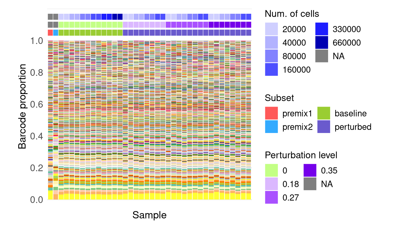

Past versions of unnamed-chunk-5-1.png

Version	Author	Date
34f5894	FeiLiyang	2026-01-01
dfa737a	FeiLiyang	2025-12-17

7 FPR

Using mixture_plus1_top data, where an offset (one) was added to the raw count, based on which proportion was calculated. However the “top” barcodes were filtered based on the raw count data.

Here we subset the 12 “null” samples for evaluating FPR of diff_prop, and diff_occ methods.

Three transformations with dif_prop were evaluated separately.

• avoid running this chunk during rendering. global_all_loops was saved from the first run.

nulls <- mixture_plus1_top[, mixture_plus1_top$sampleMetadata$Subset == "null"]

results_negsi <- suppressMessages({
  random_sampling(barbieQ = nulls, loop_times = 100)
  })

## `random_sampling()` save the simulations to global environment
## as `global_all_loops`
save(global_all_loops, file = "output/mixture_negative_simulation.rda")

results_negsi[[1]] <- results_negsi[[1]] + ggtitle("Prop_asin, perturb_null")
results_negsi[[2]] <- results_negsi[[2]] + ggtitle("Prop_logit, perturb_null")
results_negsi[[3]] <- results_negsi[[3]] + ggtitle("Prop_noTrans, perturb_null")
results_negsi[[4]] <- results_negsi[[4]] + ggtitle("Occ_firth, perturb_null")
results_negsi[[5]] <- results_negsi[[5]] + ggtitle("Prop_asin, perturb_null")
results_negsi[[6]] <- results_negsi[[6]] + ggtitle("Prop_logit, perturb_null")
results_negsi[[7]] <- results_negsi[[7]] + ggtitle("Prop_noTrans, perturb_null")
results_negsi[[8]] <- results_negsi[[8]] + ggtitle("Occ_firth, perturb_null")

wrap_plots(results_negsi[1:8], ncol = 4)

7.1 load results

## loading random sampling results to avoid running it repeatedly
load("output/mixture_negative_simulation.rda")

  # extract results from the loops
  end_sampling <- 6
  
  ## extract FPR
  all_FPR <- lapply(seq(3:end_sampling), function(n) {
    global_all_loops[[n]]$FPR
  })
  df_FPR <- do.call(rbind, all_FPR)
  
  ## extract P.Val
  all_P.Val <- lapply(seq(3:end_sampling), function(n) {
    global_all_loops[[n]]$P.Val
  })
  df_P.Val <- do.call(rbind, all_P.Val)
  
  ## extract MA
  all_MA <- lapply(seq(3:end_sampling), function(n) {
    global_all_loops[[n]]$MA
  })
  df_MA <- do.call(rbind, all_MA)
  
  all_Group_Vec <- lapply(seq(3:end_sampling), function(n) {
    global_all_loops[[n]]$Group_Vec
  })
  df_Group_Vec <- do.call(rbind, all_Group_Vec)
  
  stats_barcodes <- cbind(df_P.Val[,1:4], df_MA)

7.2 F3C: Type I Error Rate

• Diff_prop

df_FPR$N_Samples <- as.factor(df_FPR$N_Samples)
  
  ## reshape the data to fit methods for testing
df_FPR_long <- df_FPR %>%
  pivot_longer(cols = starts_with("Prop_"),
               names_to = "Method",
               values_to = "Pval_Prop") %>%
  mutate(Method = factor(Method, levels = c("Prop_asin", "Prop_logit", "Prop_noTrans"),
                         labels = c("asin-sqrt", "logit", "no trans.")))

P_FPR_add1_prop <- ggplot(
  df_FPR_long, aes(x = factor(N_Samples), y = Pval_Prop, color = Method)) +
  geom_boxplot(outlier.shape = 1, position = position_dodge(width = 0.7)) +
  # geom_jitter(size = 1, position = position_dodge(width = 0.7)) +
  geom_hline(yintercept = 0.05, linetype = "dashed", color = "black") +
  # coord_cartesian(ylim = c(0, 0.2)) + 
  labs(
       y = "Fraction of P-Value < 0.05",
       x = "Number of samples per group",
       title = "Type I error rate",
       subtitle = "Differential proportion test") +
  # facet_wrap(~Method, scales = "free_y") +
  theme_classic() +
  theme(legend.position = "top")

• Diff_occ. when converting barcode presence / absence, setting the threshold as CPM>10 instead of the default 1, as an offset (one) was added to the raw count preprocessing.

P_FPR_occ <- ggplot(
  df_FPR, aes(x = factor(N_Samples), y = Occ_firth)) +
  geom_boxplot(outlier.shape = 1, position = position_dodge(width = 0.7)) +
  # geom_jitter(size = 1, position = position_dodge(width = 0.7)) +
  geom_hline(yintercept = 0.05, linetype = "dashed", color = "black") +
  scale_color_manual(values = c("Differential occurrrence test" = "black")) +
  # coord_cartesian(ylim = c(0, 0.2)) + 
  labs(
       y = "Fraction of P-Value < 0.05",
       x = "Number of samples per group",
       titlte = "",
       subtitle = "Differential occurrence test") +
  theme_classic() +
  theme(legend.position = "top")

f3c <- (P_FPR_add1_prop + theme_barbieQ_size() + theme(legend.position = "top")) + 
  (P_FPR_occ + theme_barbieQ_size())

f3c

Ignoring unknown labels:
• titlte : ""

Warning: No shared levels found between `names(values)` of the manual scale and the
data's colour values.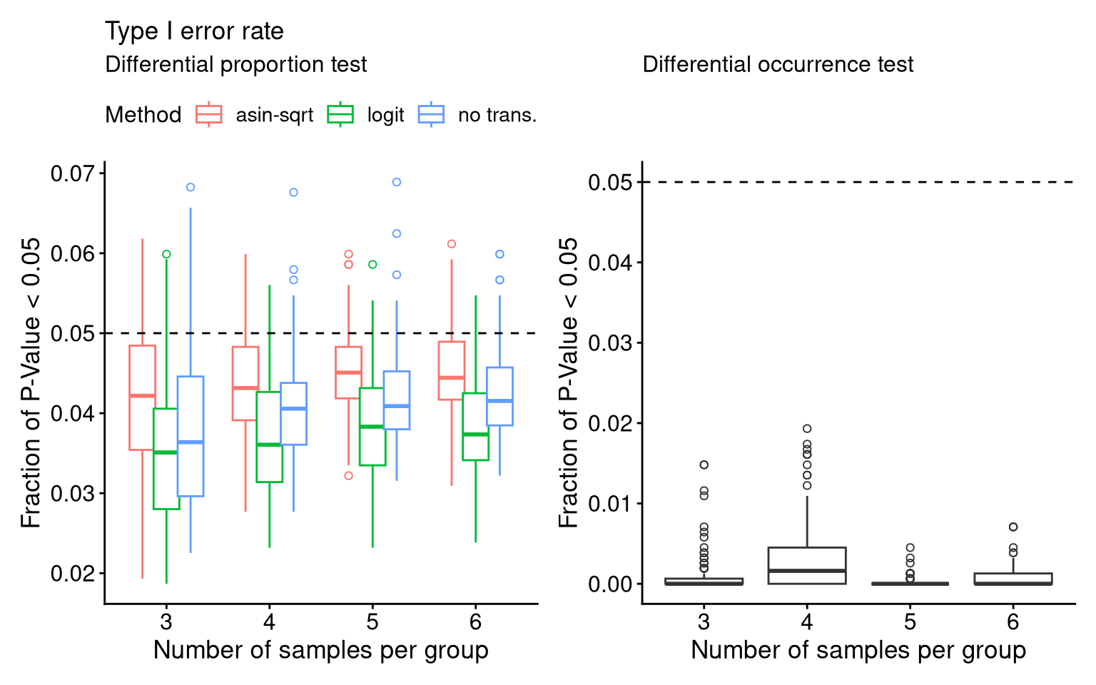

Past versions of unnamed-chunk-11-1.png

Version	Author	Date
34f5894	FeiLiyang	2026-01-01
dfa737a	FeiLiyang	2025-12-17

7.3 F3H: Type I Error Rate as a function to N_BC

7.3.1 Generate subsets of barcodes

## with different filtering thresholds, how many "top" barcodes do we get
1:9/10

[1] 0.1 0.2 0.3 0.4 0.5 0.6 0.7 0.8 0.9

lapply(
  c(1:9/10, 0.95), 
  function(filter_level) {
    mixture_plus1 <- tagTopBarcodes(mixture_plus1, nSampleThreshold = 8, proportionThreshold = filter_level)
    paste0("filter_thresh=", filter_level, "; N_barcodes=", sum(rowData(mixture_plus1)$isTopBarcode$isTop)) %>% print()
    # plotBarcodeSankey(mixture)
    
    return(
      sum(rowData(mixture_plus1)$isTopBarcode$isTop)
    )
  }
  ) %>% unlist() %>% 
  setNames(nm = c(1:9/10, 0.95)) ->
  filter_to_N

[1] "filter_thresh=0.1; N_barcodes=12"
[1] "filter_thresh=0.2; N_barcodes=32"
[1] "filter_thresh=0.3; N_barcodes=64"
[1] "filter_thresh=0.4; N_barcodes=101"
[1] "filter_thresh=0.5; N_barcodes=169"
[1] "filter_thresh=0.6; N_barcodes=269"
[1] "filter_thresh=0.7; N_barcodes=394"
[1] "filter_thresh=0.8; N_barcodes=617"
[1] "filter_thresh=0.9; N_barcodes=1060"
[1] "filter_thresh=0.95; N_barcodes=1553"

filter_to_N

 0.1  0.2  0.3  0.4  0.5  0.6  0.7  0.8  0.9 0.95 
  12   32   64  101  169  269  394  617 1060 1553 

names(filter_to_N) %>% str()

 chr [1:10] "0.1" "0.2" "0.3" "0.4" "0.5" "0.6" "0.7" "0.8" "0.9" "0.95"

7.3.2 Update proportion

## Compute medians per bin/method/N_Samples
method_labels <- c(
  "Prop_asin" = "asin-sqrt",
  "Prop_logit" = "logit",
  "Prop_noTrans" = "none"
 )

• avoid running this chunk during rendering. stats_barcodes_all_levels was saved from the first run.

stats_barcodes_all_levels <- lapply(
  c(1:9/10, 0.95),
  function(i) {
    stats_barcodes_i <- get_null_sample_by_filter(mixture_plus1, i, loop_times = 100)
    stats_barcodes_i$filter_level <- i
    stats_barcodes_i$N_BC <- filter_to_N[i %>% as.character()]
    return(stats_barcodes_i)
  }
)

stats_barcodes_all_levels <- do.call(rbind, stats_barcodes_all_levels)

save(stats_barcodes_all_levels, file = "output/fdr_by_Nbc.rda")

load("output/fdr_by_Nbc.rda")

 FPR_box <- stats_barcodes_all_levels %>%
    pivot_longer(
      cols = c(Prop_asin, Prop_logit, Prop_noTrans),
      names_to = "method",
      values_to = "pvalue"
    ) %>% 
    group_by(method, N_Samples, N_BC, Loop_N) %>%
    summarize(N_signif = sum(pvalue < 0.05), Frac_signif = sum(pvalue < 0.05) / n(), .groups = "drop") %>% 
    mutate(Method = recode(method, !!!method_labels))
  
  ggplot(FPR_box, aes(x = as.factor(N_BC), y = Frac_signif, color = Method, group = paste0(N_BC, Method))) +
    geom_boxplot(alpha = 0.6, position = position_dodge(), outliers = T) +
    labs(
      x = paste0("Number of total barcodes after filtering"),
      y = "Fraction of P-Value < 0.05", color = "Method", shape = "N_sample", linetype = "N_sample",
      title = "Type I Error Rate as a function to number of barcodes"
      ) +
    geom_hline(yintercept = 0.05, linetype = "dashed") +
    # facet_wrap(~N_Samples, ncol =4) +
    theme_linedraw()+
    theme(axis.text.x = element_text(angle = 0, vjust = 0.5, size = 10, hjust = 0.5), aspect.ratio = 0.5) + 
    theme(
        legend.title = element_text(size = 12), legend.text = element_text(size = 11),
        axis.title = element_text(size = 13), axis.text = element_text(size = 12)) + 
    scale_y_continuous(limits = c(0,0.2))

Ignoring unknown labels:
• shape : "N_sample"
• linetype : "N_sample"

Warning: Removed 80 rows containing non-finite outside the scale range
(`stat_boxplot()`).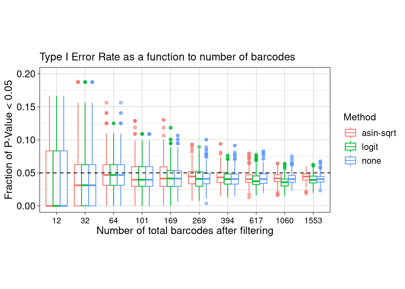

Past versions of unnamed-chunk-15-1.png

Version	Author	Date
34f5894	FeiLiyang	2026-01-01
dfa737a	FeiLiyang	2025-12-17

7.3.3 Raw proportion

## saving all p.vals from the N=1553 simulation
# df_P.Val
mixture_plus1 <- tagTopBarcodes(mixture_plus1, nSampleThreshold = 8, proportionThreshold = 0.95)
## get the subset of barcodes
lapply(c(1:9/10, 0.95), function(filter_level) {
  barbieQ <- tagTopBarcodes(mixture_plus1, nSampleThreshold = 8, proportionThreshold = filter_level)
  tag <- rowData(barbieQ)$isTopBarcode$isTop
  tag <- tag[mixture_plus1@elementMetadata$isTopBarcode$isTop]
  return(tag)
}) -> BC_set_by_filter

BC_set_by_filter <- do.call(cbind, BC_set_by_filter)
colnames(BC_set_by_filter) <- filter_to_N[c(1:9/10, 0.95) %>% as.character()]
## check
colSums(BC_set_by_filter)

  12   32   64  101  169  269  394  617 1060 1553 
  12   32   64  101  169  269  394  617 1060 1553 

mean_prop <- rowMeans(mixture_plus1[mixture_plus1@elementMetadata$isTopBarcode$isTop,mixture_plus1$sampleMetadata$Subset=="null"]@assays@data$proportion)

## testing results obtained from raw proportin in stats_barcodes
df_P.Val_filter_tag <- cbind(
  stats_barcodes,  # testing results obtained from raw proportin
  mean_prop,
  BC_set_by_filter[
    rep(
      seq_len(nrow(BC_set_by_filter)),
      length.out = nrow(stats_barcodes)
      ),
    ]
  )

Warning in data.frame(..., check.names = FALSE): row names were found from a
short variable and have been discarded

FPR_box_raw <- df_P.Val_filter_tag %>%
    pivot_longer(
      cols = c(Prop_asin, Prop_logit, Prop_noTrans),
      names_to = "method",
      values_to = "pvalue"
    ) %>% 
   pivot_longer(
     cols = as.character(filter_to_N[c(1:9/10, 0.95) %>% as.character()]),
     names_to = "N_BC",
     values_to = "selectedBy"
   ) %>% 
    group_by(method, N_Samples, Loop_N, N_BC) %>%
    summarize(
      N_signif = sum(pvalue < 0.05 & selectedBy), 
      Frac_signif = sum(pvalue < 0.05 & selectedBy) / sum(selectedBy), .groups = "drop") %>% 
    mutate(Method = recode(method, !!!method_labels))

FPR_box_raw$N_BC <- as.numeric(FPR_box_raw$N_BC)
  
ggplot(FPR_box_raw, aes(x= as.factor(N_BC), y = Frac_signif, color = Method, group = paste0(Method, N_BC))) +
    geom_boxplot(alpha = 0.6, position = position_dodge(), outliers = T) +
    labs(
      x = paste0("Number of total barcodes after filtering"),
      y = "Fraction of P-Valuev < 0.05", color = "Method", shape = "N_sample", linetype = "N_sample"
      ) +
    geom_hline(yintercept = 0.05, linetype = "dashed") +
    # facet_wrap(~N_Samples, ncol =4) +
    theme_linedraw()+
    theme(axis.text.x = element_text(angle = 0, vjust = 0.5, size = 10, hjust = 0.5), aspect.ratio = 0.5) + 
    theme_barbieQ_size() + 
    scale_y_continuous(limits = c(0,0.2)) ## y scale zoom in

Ignoring unknown labels:
• shape : "N_sample"
• linetype : "N_sample"

Warning: Removed 85 rows containing non-finite outside the scale range
(`stat_boxplot()`).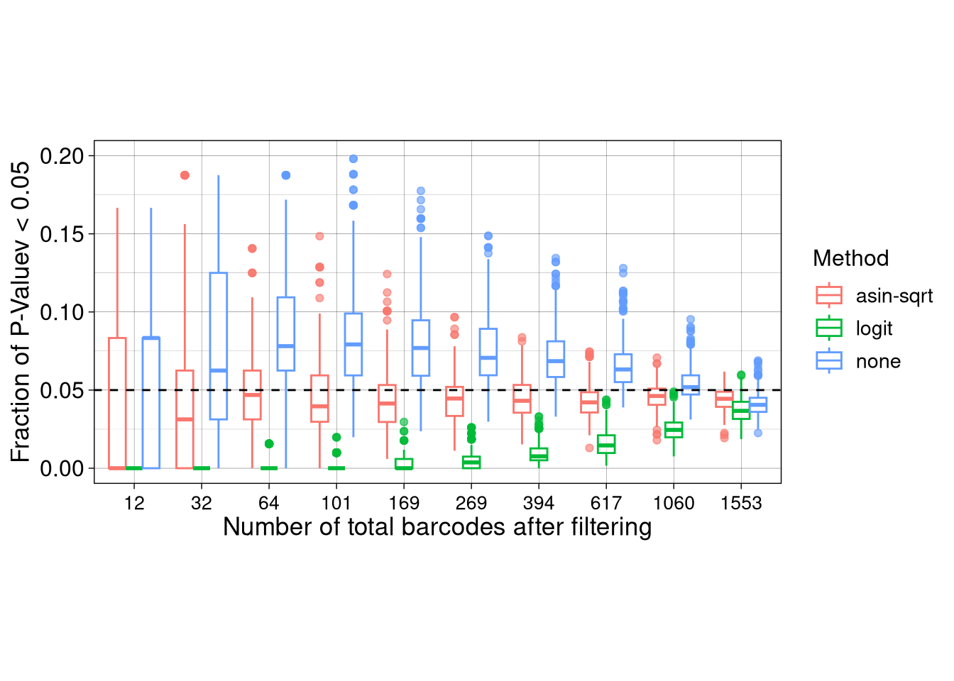

Past versions of unnamed-chunk-17-1.png

Version	Author	Date
34f5894	FeiLiyang	2026-01-01

rbind(
  data.frame(FPR_box_raw, prop_type  = "Raw proportion"), 
  data.frame(FPR_box, prop_type  = "Updated proportion")
  ) %>% 
  mutate(prop_type = factor(prop_type, levels = c("Updated proportion", "Raw proportion"))) %>% 
  ## plot
  ggplot(aes(x = as.factor(N_BC), y = Frac_signif, color = Method, group = paste0(N_BC, Method))) +
    geom_boxplot(alpha = 0.6, position = position_dodge(), outliers = T) +
    labs(
      x = paste0("Number of total barcodes after filtering"),
      y = "Fraction of P-Value < 0.05", color = "Method", shape = "N_sample", linetype = "N_sample",
      title = "Type I error rate to number of barcodes"
      ) +
  geom_hline(yintercept = 0.05, linetype = "dashed") +
  facet_grid(prop_type~1, switch = "y") +
  theme_bw()+
  theme_barbieQ_size() +
  theme(panel.grid.minor = element_blank(), axis.text.x = element_text(angle = 15, vjust = 0.5, hjust = 0.5), 
        legend.position = "top",
        strip.placement = "outside", strip.text.y = element_text(size = 12),
        strip.text.x = element_blank(), strip.background.x = element_blank()) +
  scale_y_continuous(limits = c(0,0.2)) -> f3h
  ## scale_x_discrete(limits = rev) ## reverse x axis

f3h

Ignoring unknown labels:
• shape : "N_sample"
• linetype : "N_sample"

Warning: Removed 165 rows containing non-finite outside the scale range
(`stat_boxplot()`).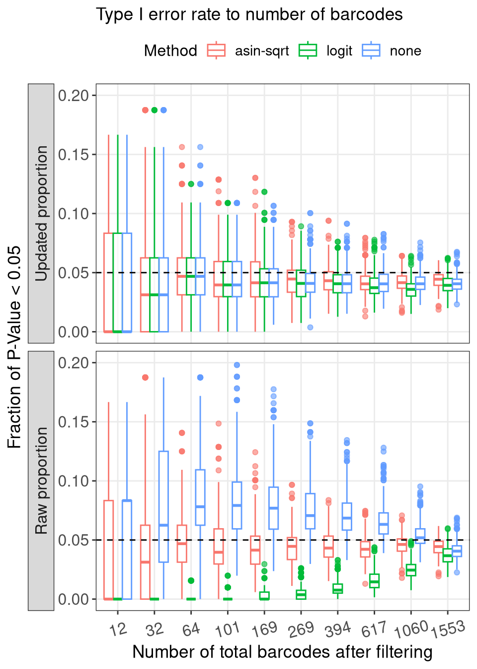

Past versions of unnamed-chunk-18-1.png

Version	Author	Date
34f5894	FeiLiyang	2026-01-01
dfa737a	FeiLiyang	2025-12-17

7.4 F3G: Density to N_Barcodes

7.4.1 Updated proportion

## get the subset of barcodes
lapply(c(1:9/10, 0.95), function(filter_level) {
  barbieQ <- tagTopBarcodes(mixture_plus1, nSampleThreshold = 8, proportionThreshold = filter_level)
  tag <- rowData(barbieQ)$isTopBarcode$isTop
  
  prop_mat <- mixture_plus1[tag,mixture_plus1$sampleMetadata$Subset=="null"]@assays@data$proportion
  ## update prop
  prop_mat <- t(t(prop_mat) / colSums(prop_mat))
  
  df <- data.frame(
    prop = as.vector(prop_mat), 
    N_BC=filter_to_N[as.character(filter_level)]
    )
  return(df)
}) -> BC_set_prop_filter

Warning in data.frame(prop = as.vector(prop_mat), N_BC =
filter_to_N[as.character(filter_level)]): row names were found from a short
variable and have been discarded
Warning in data.frame(prop = as.vector(prop_mat), N_BC =
filter_to_N[as.character(filter_level)]): row names were found from a short
variable and have been discarded
Warning in data.frame(prop = as.vector(prop_mat), N_BC =
filter_to_N[as.character(filter_level)]): row names were found from a short
variable and have been discarded
Warning in data.frame(prop = as.vector(prop_mat), N_BC =
filter_to_N[as.character(filter_level)]): row names were found from a short
variable and have been discarded
Warning in data.frame(prop = as.vector(prop_mat), N_BC =
filter_to_N[as.character(filter_level)]): row names were found from a short
variable and have been discarded
Warning in data.frame(prop = as.vector(prop_mat), N_BC =
filter_to_N[as.character(filter_level)]): row names were found from a short
variable and have been discarded
Warning in data.frame(prop = as.vector(prop_mat), N_BC =
filter_to_N[as.character(filter_level)]): row names were found from a short
variable and have been discarded
Warning in data.frame(prop = as.vector(prop_mat), N_BC =
filter_to_N[as.character(filter_level)]): row names were found from a short
variable and have been discarded
Warning in data.frame(prop = as.vector(prop_mat), N_BC =
filter_to_N[as.character(filter_level)]): row names were found from a short
variable and have been discarded
Warning in data.frame(prop = as.vector(prop_mat), N_BC =
filter_to_N[as.character(filter_level)]): row names were found from a short
variable and have been discarded

BC_set_prop_filter <- do.call(rbind, BC_set_prop_filter)

ggplot(BC_set_prop_filter) +
  geom_density(aes(x = prop, color = as.factor(N_BC), group = as.factor(N_BC))) +
  scale_x_log10(breaks = 10^seq(-6, -1, by = 1), labels = strip_zeros) +
  coord_cartesian(xlim = c(1e-6, 3e-1)) +
  labs(color = "Num. BC", x = "Barcode Proportion", y = "Density", subtitle = "with updated proportion") +
  theme_barbieQ() +
  theme(aspect.ratio = 0.9) -> f3g1

7.4.2 Raw proportion

## get the subset of barcodes
lapply(c(1:9/10, 0.95), function(filter_level) {
  barbieQ <- tagTopBarcodes(mixture_plus1, nSampleThreshold = 8, proportionThreshold = filter_level)
  tag <- rowData(barbieQ)$isTopBarcode$isTop
  ## keep raw prop
  prop_mat <- mixture_plus1[tag,mixture_plus1$sampleMetadata$Subset=="null"]@assays@data$proportion
  df <- data.frame(
    prop = as.vector(prop_mat), 
    N_BC=filter_to_N[as.character(filter_level)]
    )
  return(df)
}) -> BC_set_prop_filter_raw

Warning in data.frame(prop = as.vector(prop_mat), N_BC =
filter_to_N[as.character(filter_level)]): row names were found from a short
variable and have been discarded
Warning in data.frame(prop = as.vector(prop_mat), N_BC =
filter_to_N[as.character(filter_level)]): row names were found from a short
variable and have been discarded
Warning in data.frame(prop = as.vector(prop_mat), N_BC =
filter_to_N[as.character(filter_level)]): row names were found from a short
variable and have been discarded
Warning in data.frame(prop = as.vector(prop_mat), N_BC =
filter_to_N[as.character(filter_level)]): row names were found from a short
variable and have been discarded
Warning in data.frame(prop = as.vector(prop_mat), N_BC =
filter_to_N[as.character(filter_level)]): row names were found from a short
variable and have been discarded
Warning in data.frame(prop = as.vector(prop_mat), N_BC =
filter_to_N[as.character(filter_level)]): row names were found from a short
variable and have been discarded
Warning in data.frame(prop = as.vector(prop_mat), N_BC =
filter_to_N[as.character(filter_level)]): row names were found from a short
variable and have been discarded
Warning in data.frame(prop = as.vector(prop_mat), N_BC =
filter_to_N[as.character(filter_level)]): row names were found from a short
variable and have been discarded
Warning in data.frame(prop = as.vector(prop_mat), N_BC =
filter_to_N[as.character(filter_level)]): row names were found from a short
variable and have been discarded
Warning in data.frame(prop = as.vector(prop_mat), N_BC =
filter_to_N[as.character(filter_level)]): row names were found from a short
variable and have been discarded

BC_set_prop_filter_raw <- do.call(rbind, BC_set_prop_filter_raw)

ggplot(BC_set_prop_filter_raw) +
  geom_density(aes(x = prop, color = as.factor(N_BC), group = as.factor(N_BC))) +
  scale_x_log10(breaks = 10^seq(-6, -1, by = 1), labels = strip_zeros) +
  coord_cartesian(xlim = c(1e-6, 3e-1)) +
  theme_linedraw() +
  labs(color = "Num. BC", x = "Barcode Proportion", y = "Density", subtitle = "with raw proportion") +
  theme_barbieQ() +
  theme(aspect.ratio = 0.9) -> f3g2

rbind(
  data.frame(BC_set_prop_filter_raw, prop_type  = "Raw proportion"), 
  data.frame(BC_set_prop_filter, prop_type  = "Updated proportion")
  ) %>% 
  mutate(prop_type = factor(prop_type, levels = c("Updated proportion", "Raw proportion"))) %>% 
  ## pass to gplot
  ggplot() +
  geom_density(aes(x = prop, color = as.factor(N_BC), group = as.factor(N_BC))) +
  scale_x_log10(breaks = 10^seq(-6, -1, by = 1), labels = strip_zeros) +
  coord_cartesian(xlim = c(1e-6, 3e-1)) +
  facet_grid(prop_type~1, switch = "y") +
  labs(color = "Num. BC", x = "Barcode Proportion", y = "Density", title = "Barcode distribution in datasets") +
  theme_bw() +
  theme_barbieQ_size() +
  theme(panel.grid.minor = element_blank(), axis.text.x = element_text(angle = 15, vjust = 0.5, hjust = 0.5), 
        legend.position = "top", legend.key.size = unit(0.3, "cm"),
        legend.title = element_text(size = 11), legend.text  = element_text(size = 10), 
        strip.placement = "outside", strip.text.y = element_text(size = 12),
        strip.text.x = element_blank(), strip.background.x = element_blank()) ->  ## disable column label
  f3g
  
f3g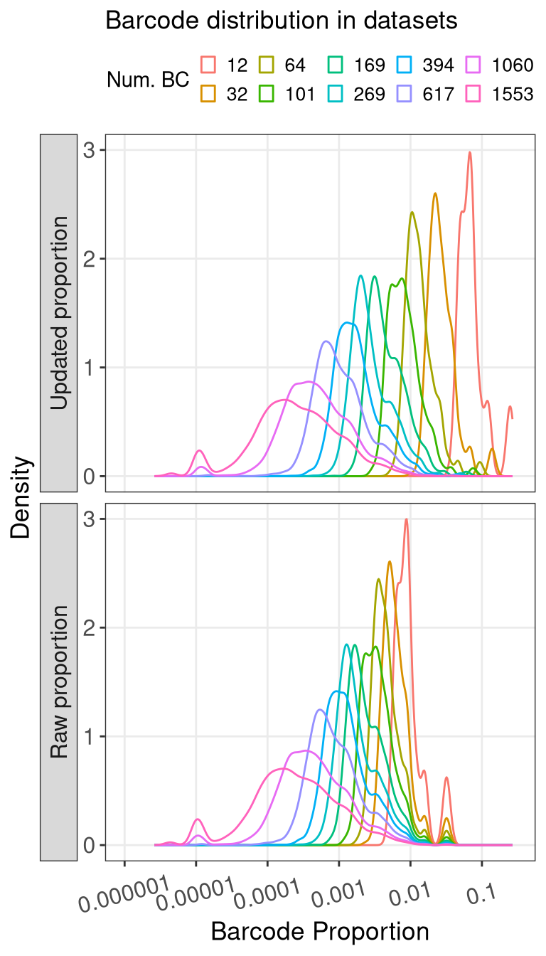

Past versions of unnamed-chunk-21-1.png

Version	Author	Date
34f5894	FeiLiyang	2026-01-01

7.5 F3D: Quantile distribution

data.frame(x = (stats_barcodes_all_levels %>% filter(filter_level==0.95))$Amean_prop) %>%
  mutate(quantile_bin = ntile(x, 10)) %>% 
  ggplot(aes(x = as.factor(quantile_bin), y = x, group = quantile_bin)) +
  geom_jitter(color = "grey", shape = ".") + 
  geom_boxplot() +
  scale_y_log10(breaks = 10^seq(-5, -1, by = 1), labels = strip_zeros) +
  theme_barbieQ() +
  labs(x = "Quantiles of barcode mean proportion", y = "Barcode mean proportion",
       title = "Barcode proportion distribution", subtitle = " ") +
  theme(axis.text.y = element_text(angle = 90, vjust = 0.5, hjust = 0.5)) -> f3d

f3d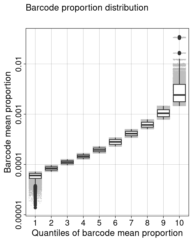

Past versions of unnamed-chunk-22-1.png

Version	Author	Date
34f5894	FeiLiyang	2026-01-01
dfa737a	FeiLiyang	2025-12-17

7.6 F3E: False positives in quantiles

• For diff_prop

# plot_fdr_on_quantile(stats_barcodes_all_levels %>% filter(filter_level==0.1), num_quantiles = 4)
# plot_fdr_on_quantile(stats_barcodes_all_levels %>% filter(filter_level==0.2), num_quantiles = 10)
# plot_fdr_on_quantile(stats_barcodes_all_levels %>% filter(filter_level==0.3), num_quantiles = 10)
# plot_fdr_on_quantile(stats_barcodes_all_levels %>% filter(filter_level==0.4), num_quantiles = 10)
# plot_fdr_on_quantile(stats_barcodes_all_levels %>% filter(filter_level==0.5), num_quantiles = 10)
# plot_fdr_on_quantile(stats_barcodes_all_levels %>% filter(filter_level==0.6), num_quantiles = 10)
# plot_fdr_on_quantile(stats_barcodes_all_levels %>% filter(filter_level==0.7), num_quantiles = 10)
# plot_fdr_on_quantile(stats_barcodes_all_levels %>% filter(filter_level==0.8), num_quantiles = 10)
# plot_fdr_on_quantile(stats_barcodes_all_levels %>% filter(filter_level==0.9), num_quantiles = 10)

plot_fdr_on_quantile(stats_barcodes_all_levels %>% filter(filter_level==0.95), num_quantiles = 10) + 
  theme_barbieQ() +
  labs(title = "Type I error rate in quanties") -> f3e

8 TPR

8.1 Check premix

• confirming an equal mixture of pool1 and pool2 in baseline samples (the “null” samples).

colnames(mixture_plus1_top)

 [1] "P1"               "P2"               "null_660.1"       "null_660.2"      
 [5] "null_330.1"       "null_330.2"       "null_160.1"       "null_160.2"      
 [9] "null_80.1"        "null_80.2"        "null_40.1"        "null_40.2"       
[13] "null_20.1"        "null_20.2"        "m_null_160.p35.1" "m_null_160.p27.1"
[17] "m_null_160.p18.1" "m_null_160.p35.2" "m_null_160.p27.2" "m_null_160.p18.2"
[21] "m_null_80.p35.1"  "m_null_80.p27.1"  "m_null_80.p18.1"  "m_null_80.p35.2" 
[25] "m_null_80.p27.2"  "m_null_80.p18.2"  "m_null_40.p35.1"  "m_null_40.p27.1" 
[29] "m_null_40.p18.1"  "m_null_40.p35.2"  "m_null_40.p27.2"  "m_null_40.p18.2" 
[33] "m_null_20.p35.1"  "m_null_20.p27.1"  "m_null_20.p18.1"  "m_null_20.p35.2" 
[37] "m_null_20.p27.2"  "m_null_20.p18.2" 

prop_raw <- mixture_plus1_top@assays@data$proportion

pool1_vec <- prop_raw[,1]
pool2_vec <- prop_raw[,2]

## if equal mixture of pool1 and pool2; designed prop should be 1/2 of total props in original pool1 and pool2 
check_mix_df <- data.frame(
  ps = rowMeans(prop_raw[,1:2]), 
  mixture_660 = prop_raw[,3]
  )

ggplot(check_mix_df, aes(x = ps, y = mixture_660)) + 
  geom_point() + 
  coord_fixed() +
  geom_smooth(method = "lm")

`geom_smooth()` using formula = 'y ~ x'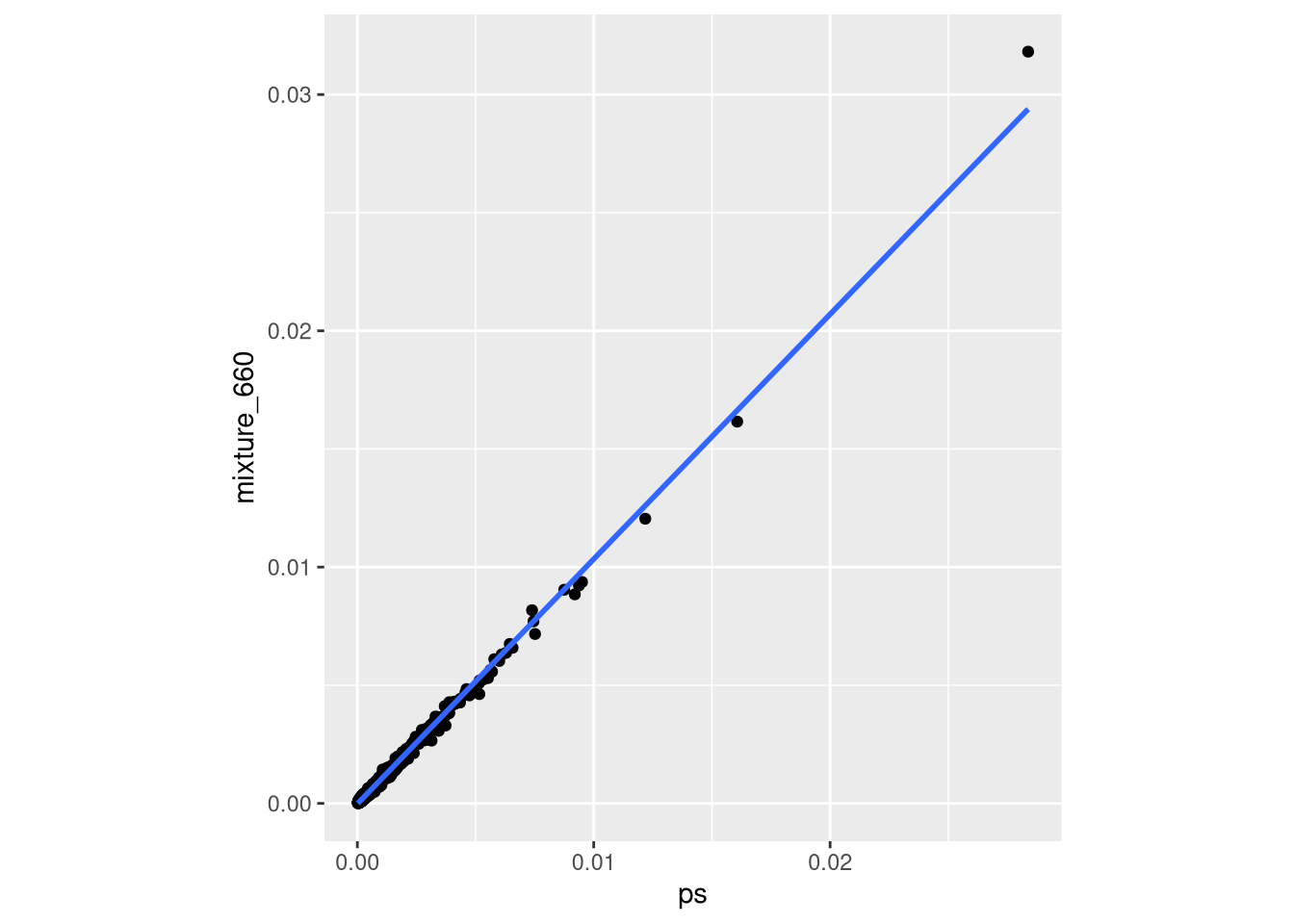

Past versions of unnamed-chunk-24-1.png

Version	Author	Date
34f5894	FeiLiyang	2026-01-01
dfa737a	FeiLiyang	2025-12-17

• Confirming orthogonal between premix1 and premix2: barcodes mostly not overlapping between the two premix samples, but a few noise are observed in premix2.

ggplot(data.frame(prop_raw) %>% sqrt() %>% asin()) + 
  geom_point(aes(x = P1, y = P2))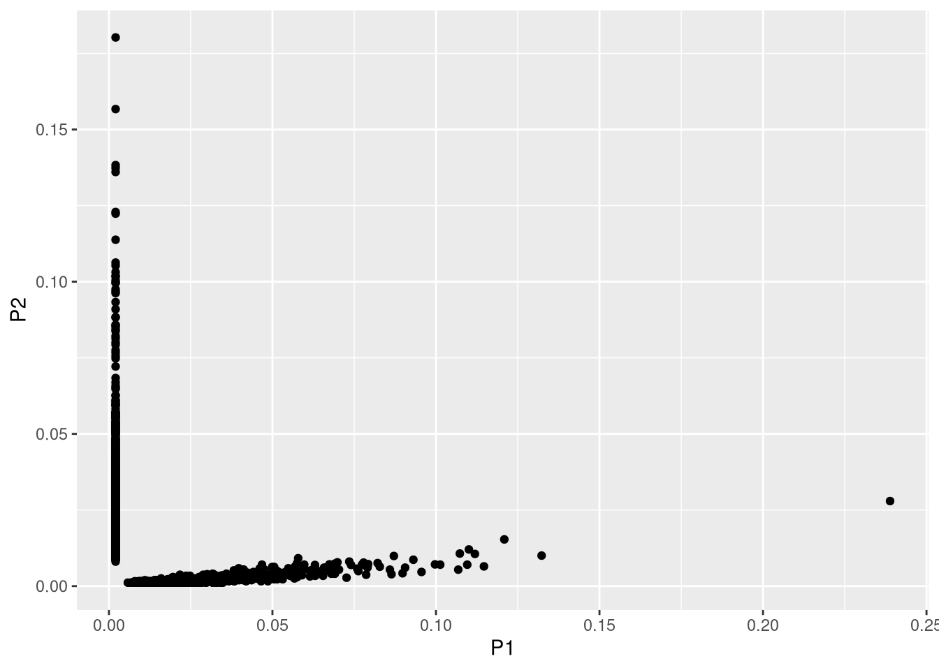

Past versions of unnamed-chunk-25-1.png

Version	Author	Date
34f5894	FeiLiyang	2026-01-01
a2e7a36	FeiLiyang	2025-12-17

ggplot(data.frame(prop_raw) %>% sqrt() %>% asin(), aes(x = P1+P2, y = abs(P1-P2))) + 
  geom_point() +
  coord_fixed() +
  geom_smooth(method = "lm")

`geom_smooth()` using formula = 'y ~ x'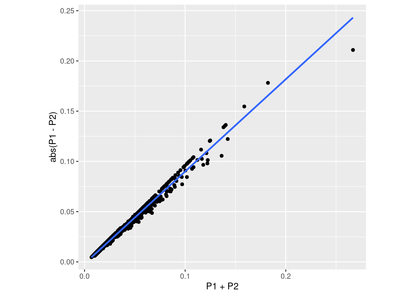

Past versions of unnamed-chunk-25-2.png

Version	Author	Date
34f5894	FeiLiyang	2026-01-01

ggplot(data.frame(prop_raw), aes(x = P1+P2, y = abs(P1-P2))) + 
  geom_point() +
  coord_fixed() +
  geom_smooth(method = "lm")

`geom_smooth()` using formula = 'y ~ x'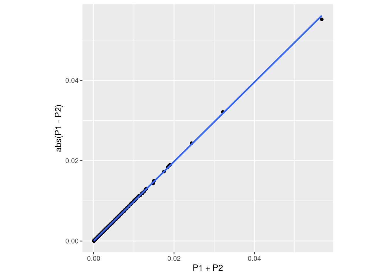

Past versions of unnamed-chunk-25-3.png

Version	Author	Date
34f5894	FeiLiyang	2026-01-01

8.2 Designed differences

## theory
a = 0.35
((1/2 + a) / (1+a)) - (1/2)

[1] 0.1296296

a = 0.27
(1/2 + a) / (1+a) - 1/2

[1] 0.1062992

a = 0.18
(1/2 + a) / (1+a) - 1/2

[1] 0.07627119

8.3 Model perturbations

mixture_plus1_top$sampleMetadata %>% as.data.frame() %>% summary()

     Subset    BarcodeSize      Perturbation    TechRep
 premix1: 1   Min.   : 20000   Min.   :0.0000   1:20   
 premix2: 1   1st Qu.: 40000   1st Qu.:0.0000   2:18   
 null   :12   Median : 80000   Median :0.1800          
 perturb:24   Mean   :121667   Mean   :0.1778          
              3rd Qu.:160000   3rd Qu.:0.2700          
              Max.   :660000   Max.   :0.3500          
              NA's   :2        NA's   :2               

mixed <- mixture_plus1_top[, mixture_plus1_top$sampleMetadata$Subset %in% c("perturb", "null")]
mixed$sampleMetadata %>% as.data.frame() %>%  data.table()

mixed_target <- mixed$sampleMetadata %>% as.data.frame()
## factorize perturbation levels and barcodeSize levels
mixed_target$Perturbation <- as.factor(mixed_target$Perturbation)
levels(mixed_target$Perturbation)

[1] "0"    "0.18" "0.27" "0.35"

mixed_target$BarcodeSize <- as.factor(mixed_target$BarcodeSize)
levels(mixed_target$BarcodeSize)

[1] "20000"  "40000"  "80000"  "160000" "330000" "660000"

mixed_design <- mixed_target %>%
    with(model.matrix(~0 + Perturbation + BarcodeSize))

myblock <- mixed_target %>% with(paste(BarcodeSize, Perturbation))
table(myblock)

myblock
   160000 0 160000 0.18 160000 0.27 160000 0.35     20000 0  20000 0.18 
          2           2           2           2           2           2 
 20000 0.27  20000 0.35    330000 0     40000 0  40000 0.18  40000 0.27 
          2           2           2           2           2           2 
 40000 0.35    660000 0     80000 0  80000 0.18  80000 0.27  80000 0.35 
          2           2           2           2           2           2 

8.4 Apply tests: extract estimates

myblock <- NULL

es_de_none <- lapply(c(0.18, 0.27, 0.35), function(i) apply_model(mixed, mixed_design, myblock, a = i))

setting Perturbation as the primary factor in `sampleMetadata`.

no block specified, so there are no duplicate measurements.

setting Perturbation as the primary factor in `sampleMetadata`.

no block specified, so there are no duplicate measurements.

setting Perturbation as the primary factor in `sampleMetadata`.

no block specified, so there are no duplicate measurements.

es_de_none_df <- do.call(rbind, es_de_none)
es_de_none_df <- es_de_none_df %>% 
  mutate(Signif. = ifelse(P.Value<0.05, "signif.", "n.s.")) %>% 
  mutate(Signif. = factor(Signif., levels = c("signif.", "n.s.")))

es_de_asin <- lapply(c(0.18, 0.27, 0.35), function(i) apply_model(mixed, mixed_design, myblock, a = i, trans = "asin-sqrt"))

setting Perturbation as the primary factor in `sampleMetadata`.
no block specified, so there are no duplicate measurements.

setting Perturbation as the primary factor in `sampleMetadata`.

no block specified, so there are no duplicate measurements.

setting Perturbation as the primary factor in `sampleMetadata`.

no block specified, so there are no duplicate measurements.

es_de_asin_df <- do.call(rbind, es_de_asin)
es_de_asin_df <- es_de_asin_df %>% 
  mutate(Signif. = ifelse(P.Value<0.05, "signif.", "n.s.")) %>% 
  mutate(Signif. = factor(Signif., levels = c("signif.", "n.s.")))

es_de_logit <- lapply(c(0.18, 0.27, 0.35), function(i) apply_model(mixed, mixed_design, myblock, a = i, trans = "logit"))

setting Perturbation as the primary factor in `sampleMetadata`.
no block specified, so there are no duplicate measurements.

setting Perturbation as the primary factor in `sampleMetadata`.

no block specified, so there are no duplicate measurements.

setting Perturbation as the primary factor in `sampleMetadata`.

no block specified, so there are no duplicate measurements.

es_de_logit_df <- do.call(rbind, es_de_logit)
es_de_logit_df <- es_de_logit_df %>% 
  mutate(Signif. = ifelse(P.Value<0.05, "signif.", "n.s.")) %>% 
  mutate(Signif. = factor(Signif., levels = c("signif.", "n.s.")))

es_de_df <- rbind(es_de_none_df, es_de_asin_df, es_de_logit_df)

8.5 FS3A: Validate estimates

regression_stats_none <- es_de_none_df %>%
  group_by(Contrast) %>%
  summarise(
    cor = cor(diff, meanDiff),
    slope = coef(lm(meanDiff ~ I(diff)))[2],
    interc = coef(lm(meanDiff ~ I(diff)))[1],
    # res = resid(mod <- lm(meanDiff ~ I(diff))),
    # meanDiff = meanDiff,
    .groups = "drop"
  )
regression_stats_none$Method = "none"
regression_stats_none$x = -0.01
regression_stats_none$y = 0.01

regression_stats_asin <- es_de_asin_df %>%
  group_by(Contrast) %>%
  summarise(
    cor = cor(diff, meanDiff),
    slope = coef(lm((meanDiff) ~ I(diff)))[2],
    interc = coef(lm((meanDiff) ~ I(diff)))[1],
    .groups = "drop"
  )
regression_stats_asin$Method = "asin-sqrt"
regression_stats_asin$x = -0.001
regression_stats_asin$y = 0.001


regression_stats_logit <- es_de_logit_df %>%
  group_by(Contrast) %>%
  summarise(
    cor = cor(diff, (meanDiff)),
    slope = coef(lm((meanDiff) ~ I(diff)))[2],
    interc = coef(lm((meanDiff) ~ I(diff)))[1],
    .groups = "drop"
  )
regression_stats_logit$Method = "logit"
regression_stats_logit$x = -0.05
regression_stats_logit$y = 1

regression_stats <- rbind(regression_stats_asin, regression_stats_none, regression_stats_logit)

(facet_grid doesn’t allow free x sclae for the same column. so plot three methods seperately.)

p_es_de_asin <- ggplot(es_de_asin_df, aes(x = diff, y = (meanDiff))) +
  geom_point(aes(color = Signif.), alpha = 0.5) +
  # stat_smooth(method = "lm", linetype = "dashed", colour = "black") +
    geom_abline(data = regression_stats_none, aes(intercept = interc, slope = slope), linetype = "dashed") +
  theme_bw() +
  # coord_fixed() +
  facet_wrap(~paste0("Contrast: ", Contrast)) +
  geom_text(data = regression_stats_asin, x = -0.01, y = 0.01, 
            aes(label = paste0("r = ", round(cor, digits = 2), "\n", "slope = ", round(slope, digits = 2)))) + 
  theme(axis.title.x = element_blank(), legend.position = "none") +
  labs(color = "Barcode", y = " \n \n (asin-sqrt)")


p_es_de_none <- ggplot(es_de_none_df, aes(x = diff, y = (meanDiff))) +
  geom_point(aes(color = Signif.), alpha = 0.5) +
  # stat_smooth(method = "lm", linetype = "dashed", colour = "black") +
  geom_abline(data = regression_stats_none, aes(intercept = interc, slope = slope), linetype = "dashed") +
  theme_linedraw()+
  # coord_fixed() +
  facet_wrap(~paste0("Contrast: ", Contrast)) +
    geom_text(data = regression_stats_none, x = -0.0015, y = 0.001, 
            aes(label = paste0("r = ", round(cor, digits = 2), "\n", "slope = ", round(slope, digits = 2)))) + 
  labs(y = " \n \n (no transformation)", x = " \n Designed differences")+
  ## zoom in, removing a few barcodes with large proportion. 
  scale_x_continuous(limits = c(-0.003, 0.003)) +
  scale_y_continuous(limits = c(-0.003, 0.003)) +
  theme(legend.position = "none", strip.text = element_blank()) + # remove facet titles
  labs(color = "Barcode")

p_es_de_logit <- ggplot(es_de_logit_df, aes(x = diff, y = (meanDiff))) +
  geom_point(aes(color = Signif.), alpha = 0.5) +
  # stat_smooth(method = "lm", linetype = "dashed", colour = "black") +
  geom_abline(data = regression_stats_none, aes(intercept = interc, slope = slope), linetype = "dashed") +
  theme_linedraw()+
  facet_wrap(~paste0("Contrast: ", Contrast)) +
    geom_text(data = regression_stats_logit, x = -0.15, y = 1, 
            aes(label = paste0("r = ", round(cor, digits = 2), "\n", "slope = ", round(slope, digits = 2)))) + 
  labs(y = "Estimated differences \n \n (logit)", color = "Barcode") +
   ## zoom in, removing one barcode with large proportion. 
  # scale_x_continuous(limits = c(-0.3, 0.3)) +
  # scale_y_continuous(limits = c(-0.3, 0.3)) +
  theme(axis.title.x = element_blank(), legend.position = "right", strip.text = element_blank())  # remove facet titles

fs3a <- (p_es_de_asin + theme(legend.title = element_text(size = 12), legend.text = element_text(size = 11),
        axis.title = element_text(size = 13), axis.text = element_text(size = 12)) ) / 
  (p_es_de_logit + theme(legend.title = element_text(size = 12), legend.text = element_text(size = 11),
        axis.title = element_text(size = 13), axis.text = element_text(size = 12))) /
  (p_es_de_none + theme(legend.title = element_text(size = 12), legend.text = element_text(size = 11),
        axis.title = element_text(size = 13), axis.text = element_text(size = 12))) 
fs3a

Warning: Removed 7 rows containing missing values or values outside the scale range
(`geom_point()`).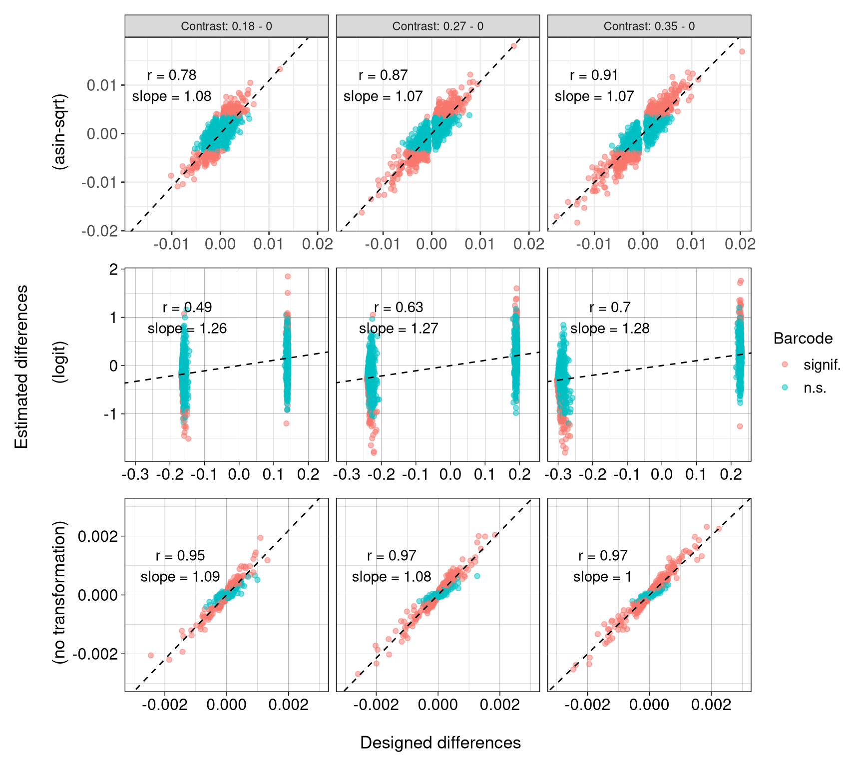

Past versions of unnamed-chunk-32-1.png

Version	Author	Date
34f5894	FeiLiyang	2026-01-01
dfa737a	FeiLiyang	2025-12-17

8.6 F3I: TPR as a function to N_BC

8.6.1 Updated proportion

test_perturb <- function(mixed, mixed_target, mixed_design, myblock, trans = "none", a = 0.18) {
  tester <- testBarcodeSignif(
    barbieQ = mixed, sampleMetadata = mixed_target, sampleGroup = "Perturbation", 
    contrastFormula = paste0("Perturbation", a, " - Perturbation0"), transformation = trans,
    designMatrix = mixed_design, block = myblock)
  
  veri_diff <- as.data.frame(tester@elementMetadata$testingBarcode)
  
  veri_diff <- rownames_to_column(veri_diff, var = "BC") 
  veri_diff$Contrast = paste0(a, " - 0")
  veri_diff$Method = trans

  
  return(veri_diff)
}

test_all_levels <- lapply(
  c(1:9/10, 0.95),
  function(i) {get_mixted_by_filter(barbieQ = mixture_plus1, filter_level = i)}
)

setting Perturbation as the primary factor in `sampleMetadata`.

no block specified, so there are no duplicate measurements.

setting Perturbation as the primary factor in `sampleMetadata`.

no block specified, so there are no duplicate measurements.

setting Perturbation as the primary factor in `sampleMetadata`.

no block specified, so there are no duplicate measurements.

setting Perturbation as the primary factor in `sampleMetadata`.

no block specified, so there are no duplicate measurements.

setting Perturbation as the primary factor in `sampleMetadata`.

no block specified, so there are no duplicate measurements.

setting Perturbation as the primary factor in `sampleMetadata`.

no block specified, so there are no duplicate measurements.

setting Perturbation as the primary factor in `sampleMetadata`.

no block specified, so there are no duplicate measurements.

setting Perturbation as the primary factor in `sampleMetadata`.

no block specified, so there are no duplicate measurements.

setting Perturbation as the primary factor in `sampleMetadata`.

no block specified, so there are no duplicate measurements.

setting Perturbation as the primary factor in `sampleMetadata`.

no block specified, so there are no duplicate measurements.

setting Perturbation as the primary factor in `sampleMetadata`.

no block specified, so there are no duplicate measurements.

setting Perturbation as the primary factor in `sampleMetadata`.

no block specified, so there are no duplicate measurements.

setting Perturbation as the primary factor in `sampleMetadata`.

no block specified, so there are no duplicate measurements.

setting Perturbation as the primary factor in `sampleMetadata`.

no block specified, so there are no duplicate measurements.

setting Perturbation as the primary factor in `sampleMetadata`.

no block specified, so there are no duplicate measurements.

setting Perturbation as the primary factor in `sampleMetadata`.

no block specified, so there are no duplicate measurements.

setting Perturbation as the primary factor in `sampleMetadata`.

no block specified, so there are no duplicate measurements.

setting Perturbation as the primary factor in `sampleMetadata`.

no block specified, so there are no duplicate measurements.

setting Perturbation as the primary factor in `sampleMetadata`.

no block specified, so there are no duplicate measurements.

setting Perturbation as the primary factor in `sampleMetadata`.

no block specified, so there are no duplicate measurements.

setting Perturbation as the primary factor in `sampleMetadata`.

no block specified, so there are no duplicate measurements.

setting Perturbation as the primary factor in `sampleMetadata`.

no block specified, so there are no duplicate measurements.

setting Perturbation as the primary factor in `sampleMetadata`.

no block specified, so there are no duplicate measurements.

setting Perturbation as the primary factor in `sampleMetadata`.

no block specified, so there are no duplicate measurements.

setting Perturbation as the primary factor in `sampleMetadata`.

no block specified, so there are no duplicate measurements.

setting Perturbation as the primary factor in `sampleMetadata`.

no block specified, so there are no duplicate measurements.

setting Perturbation as the primary factor in `sampleMetadata`.

no block specified, so there are no duplicate measurements.

setting Perturbation as the primary factor in `sampleMetadata`.

no block specified, so there are no duplicate measurements.

setting Perturbation as the primary factor in `sampleMetadata`.

no block specified, so there are no duplicate measurements.

setting Perturbation as the primary factor in `sampleMetadata`.

no block specified, so there are no duplicate measurements.

setting Perturbation as the primary factor in `sampleMetadata`.

no block specified, so there are no duplicate measurements.

setting Perturbation as the primary factor in `sampleMetadata`.

no block specified, so there are no duplicate measurements.

setting Perturbation as the primary factor in `sampleMetadata`.

no block specified, so there are no duplicate measurements.

setting Perturbation as the primary factor in `sampleMetadata`.

no block specified, so there are no duplicate measurements.

setting Perturbation as the primary factor in `sampleMetadata`.

no block specified, so there are no duplicate measurements.

setting Perturbation as the primary factor in `sampleMetadata`.

no block specified, so there are no duplicate measurements.

setting Perturbation as the primary factor in `sampleMetadata`.

no block specified, so there are no duplicate measurements.

setting Perturbation as the primary factor in `sampleMetadata`.

no block specified, so there are no duplicate measurements.

setting Perturbation as the primary factor in `sampleMetadata`.

no block specified, so there are no duplicate measurements.

setting Perturbation as the primary factor in `sampleMetadata`.

no block specified, so there are no duplicate measurements.

setting Perturbation as the primary factor in `sampleMetadata`.

no block specified, so there are no duplicate measurements.

setting Perturbation as the primary factor in `sampleMetadata`.

no block specified, so there are no duplicate measurements.

setting Perturbation as the primary factor in `sampleMetadata`.

no block specified, so there are no duplicate measurements.

setting Perturbation as the primary factor in `sampleMetadata`.

no block specified, so there are no duplicate measurements.

setting Perturbation as the primary factor in `sampleMetadata`.

no block specified, so there are no duplicate measurements.

setting Perturbation as the primary factor in `sampleMetadata`.

no block specified, so there are no duplicate measurements.

setting Perturbation as the primary factor in `sampleMetadata`.

no block specified, so there are no duplicate measurements.

setting Perturbation as the primary factor in `sampleMetadata`.

no block specified, so there are no duplicate measurements.

setting Perturbation as the primary factor in `sampleMetadata`.

no block specified, so there are no duplicate measurements.

setting Perturbation as the primary factor in `sampleMetadata`.

no block specified, so there are no duplicate measurements.

setting Perturbation as the primary factor in `sampleMetadata`.

no block specified, so there are no duplicate measurements.

setting Perturbation as the primary factor in `sampleMetadata`.

no block specified, so there are no duplicate measurements.

setting Perturbation as the primary factor in `sampleMetadata`.

no block specified, so there are no duplicate measurements.

setting Perturbation as the primary factor in `sampleMetadata`.

no block specified, so there are no duplicate measurements.

setting Perturbation as the primary factor in `sampleMetadata`.

no block specified, so there are no duplicate measurements.

setting Perturbation as the primary factor in `sampleMetadata`.

no block specified, so there are no duplicate measurements.

setting Perturbation as the primary factor in `sampleMetadata`.

no block specified, so there are no duplicate measurements.

setting Perturbation as the primary factor in `sampleMetadata`.

no block specified, so there are no duplicate measurements.

setting Perturbation as the primary factor in `sampleMetadata`.

no block specified, so there are no duplicate measurements.

setting Perturbation as the primary factor in `sampleMetadata`.

no block specified, so there are no duplicate measurements.

setting Perturbation as the primary factor in `sampleMetadata`.

no block specified, so there are no duplicate measurements.

setting Perturbation as the primary factor in `sampleMetadata`.

no block specified, so there are no duplicate measurements.

setting Perturbation as the primary factor in `sampleMetadata`.

no block specified, so there are no duplicate measurements.

setting Perturbation as the primary factor in `sampleMetadata`.

no block specified, so there are no duplicate measurements.

setting Perturbation as the primary factor in `sampleMetadata`.

no block specified, so there are no duplicate measurements.

setting Perturbation as the primary factor in `sampleMetadata`.

no block specified, so there are no duplicate measurements.

setting Perturbation as the primary factor in `sampleMetadata`.

no block specified, so there are no duplicate measurements.

setting Perturbation as the primary factor in `sampleMetadata`.

no block specified, so there are no duplicate measurements.

setting Perturbation as the primary factor in `sampleMetadata`.

no block specified, so there are no duplicate measurements.

setting Perturbation as the primary factor in `sampleMetadata`.

no block specified, so there are no duplicate measurements.

setting Perturbation as the primary factor in `sampleMetadata`.

no block specified, so there are no duplicate measurements.

setting Perturbation as the primary factor in `sampleMetadata`.

no block specified, so there are no duplicate measurements.

setting Perturbation as the primary factor in `sampleMetadata`.

no block specified, so there are no duplicate measurements.

setting Perturbation as the primary factor in `sampleMetadata`.

no block specified, so there are no duplicate measurements.

setting Perturbation as the primary factor in `sampleMetadata`.

no block specified, so there are no duplicate measurements.

setting Perturbation as the primary factor in `sampleMetadata`.

no block specified, so there are no duplicate measurements.

setting Perturbation as the primary factor in `sampleMetadata`.

no block specified, so there are no duplicate measurements.

setting Perturbation as the primary factor in `sampleMetadata`.

no block specified, so there are no duplicate measurements.

setting Perturbation as the primary factor in `sampleMetadata`.

no block specified, so there are no duplicate measurements.

setting Perturbation as the primary factor in `sampleMetadata`.

no block specified, so there are no duplicate measurements.

setting Perturbation as the primary factor in `sampleMetadata`.

no block specified, so there are no duplicate measurements.

setting Perturbation as the primary factor in `sampleMetadata`.

no block specified, so there are no duplicate measurements.

setting Perturbation as the primary factor in `sampleMetadata`.

no block specified, so there are no duplicate measurements.

setting Perturbation as the primary factor in `sampleMetadata`.

no block specified, so there are no duplicate measurements.

setting Perturbation as the primary factor in `sampleMetadata`.

no block specified, so there are no duplicate measurements.

setting Perturbation as the primary factor in `sampleMetadata`.

no block specified, so there are no duplicate measurements.

setting Perturbation as the primary factor in `sampleMetadata`.

no block specified, so there are no duplicate measurements.

setting Perturbation as the primary factor in `sampleMetadata`.

no block specified, so there are no duplicate measurements.

setting Perturbation as the primary factor in `sampleMetadata`.

no block specified, so there are no duplicate measurements.

setting Perturbation as the primary factor in `sampleMetadata`.

no block specified, so there are no duplicate measurements.

test_all_levels <- do.call(rbind, test_all_levels)

test_TPR <- test_all_levels %>% 
  group_by(Method, Contrast, N_BC) %>% 
  summarize(Frac_signif = sum(P.Value < 0.05) / n(), .groups = "drop")

ggplot(test_TPR, aes(x = as.factor(N_BC), y = Frac_signif, color = Method, linetype = Contrast, shape = Contrast)) +
  # geom_boxplot(alpha = 0.6, position = position_dodge(), outliers = T) +
  geom_line(aes(group = paste0(Contrast, Method))) +
  geom_point() +
    labs(
      x = paste0("Number of total barcodes after filtering"),
      y = "Fraction of P-Value < 0.05",
      title = "True postive rate as a function to total barcode number"
      ) +
    geom_hline(yintercept = 0.05, linetype = "dashed") +
    theme_linedraw()+
    theme(axis.text.x = element_text(angle = 0, vjust = 0.5, size = 10, hjust = 0.5), aspect.ratio = 0.5) + 
    theme(
        legend.title = element_text(size = 12), legend.text = element_text(size = 11),
        axis.title = element_text(size = 13), axis.text = element_text(size = 12))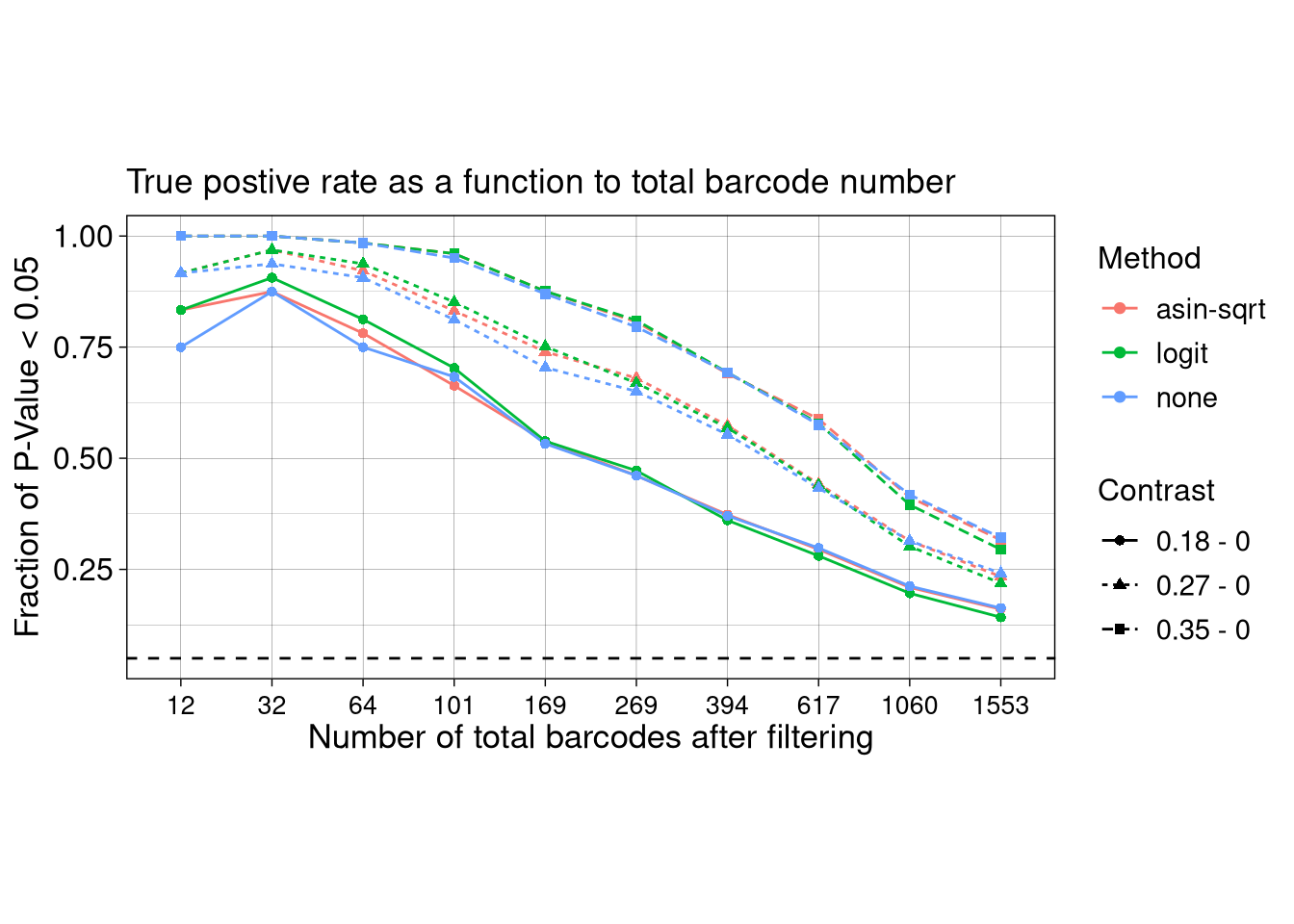

Past versions of unnamed-chunk-35-1.png

Version	Author	Date
34f5894	FeiLiyang	2026-01-01

8.6.2 Raw proportion

## test on raw proportion
test_0.95_raw <- get_mixted_by_filter(barbieQ = mixture_plus1, filter_level = 0.95, update_prop = FALSE)

setting Perturbation as the primary factor in `sampleMetadata`.

no block specified, so there are no duplicate measurements.

setting Perturbation as the primary factor in `sampleMetadata`.

no block specified, so there are no duplicate measurements.

setting Perturbation as the primary factor in `sampleMetadata`.

no block specified, so there are no duplicate measurements.

setting Perturbation as the primary factor in `sampleMetadata`.

no block specified, so there are no duplicate measurements.

setting Perturbation as the primary factor in `sampleMetadata`.

no block specified, so there are no duplicate measurements.

setting Perturbation as the primary factor in `sampleMetadata`.

no block specified, so there are no duplicate measurements.

setting Perturbation as the primary factor in `sampleMetadata`.

no block specified, so there are no duplicate measurements.

setting Perturbation as the primary factor in `sampleMetadata`.

no block specified, so there are no duplicate measurements.

setting Perturbation as the primary factor in `sampleMetadata`.

no block specified, so there are no duplicate measurements.

test_all_levels_raw <- cbind(
  test_0.95_raw,  
  mean_prop,
  BC_set_by_filter[
    rep(
      seq_len(nrow(BC_set_by_filter)),
      length.out = nrow(test_0.95_raw)
      ), 
    ]
  )

Warning in data.frame(..., check.names = FALSE): row names were found from a
short variable and have been discarded

test_TPR_raw <- test_all_levels_raw %>%
   select(-N_BC) %>% 
   pivot_longer(
     cols = as.character(filter_to_N[c(1:9/10, 0.95) %>% as.character()]),
     names_to = "N_BC",
     values_to = "selectedBy"
   ) %>% 
    group_by(Method, Contrast, N_BC) %>% 
    summarize(Frac_signif = sum(P.Value < 0.05 & selectedBy) / sum(selectedBy), .groups = "drop")

test_TPR_raw$N_BC <- as.numeric(test_TPR_raw$N_BC)

ggplot(test_TPR_raw, aes(x = as.factor(N_BC), y = Frac_signif, color = Method, group = paste0(Method, Contrast))) +
  # geom_boxplot(alpha = 0.6, position = position_dodge(), outliers = T) +
  geom_point(aes(shape = Contrast)) +
  geom_line(aes(linetype = Contrast)) +
    labs(
      x = paste0("Number of total barcodes after filtering"),
      y = "Fraction of P-Value < 0.05"
      ) +
    geom_hline(yintercept = 0.05, linetype = "dashed") +
    # facet_wrap(~Contrast, ncol =3) +
    theme_linedraw()+
    theme(axis.text.x = element_text(angle = 0, vjust = 0.5, size = 10, hjust = 0.5), aspect.ratio = 0.5) + 
    theme(
        legend.title = element_text(size = 12), legend.text = element_text(size = 11),
        axis.title = element_text(size = 13), axis.text = element_text(size = 12))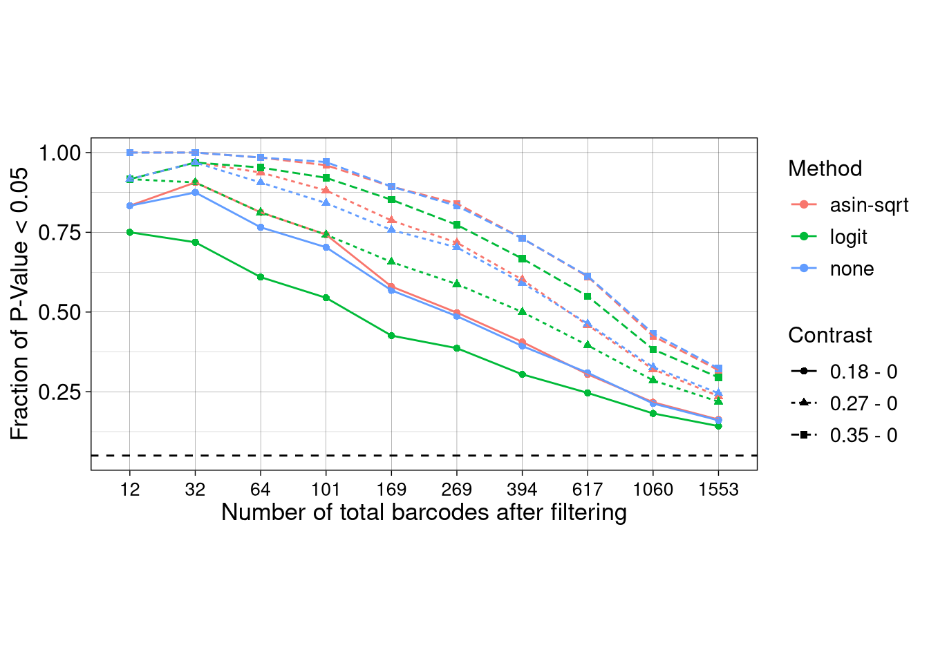

Past versions of unnamed-chunk-36-1.png

Version	Author	Date
34f5894	FeiLiyang	2026-01-01
a2e7a36	FeiLiyang	2025-12-17

rbind(
  data.frame(test_TPR_raw, prop_type  = "Raw proportion"), 
  data.frame(test_TPR, prop_type  = "Updated proportion")
  ) %>% 
  mutate(prop_type = factor(prop_type, levels = c("Updated proportion", "Raw proportion"))) %>% 
  ## plot
  ggplot(aes(x = as.factor(N_BC), y = Frac_signif, color = Method, group = paste0(Method, Contrast))) +
  # geom_boxplot(alpha = 0.6, position = position_dodge(), outliers = T) +
  geom_point(aes(shape = Contrast)) +
  geom_line(aes(linetype = Contrast)) +
    labs(
      x = paste0("Number of total barcodes after filtering"),
      y = "Fraction of P-Value < 0.05", color = "Method", shape = "Contrast", linetype = "Contrast",
      title = "True positive rate to number of barcodes"
      ) +
  geom_hline(yintercept = 0.05, linetype = "dashed") +
  facet_grid(prop_type~1, switch = "y") +
  theme_bw()+
  theme_barbieQ_size() +
  theme(panel.grid.minor = element_blank(), axis.text.x = element_text(angle = 15, vjust = 0.5, hjust = 0.5), 
        legend.position = "top",
        strip.placement = "outside", strip.text.y = element_text(size = 12),
        strip.text.x = element_blank(), strip.background.x = element_blank()) + guides(color = "none") -> f3i

f3i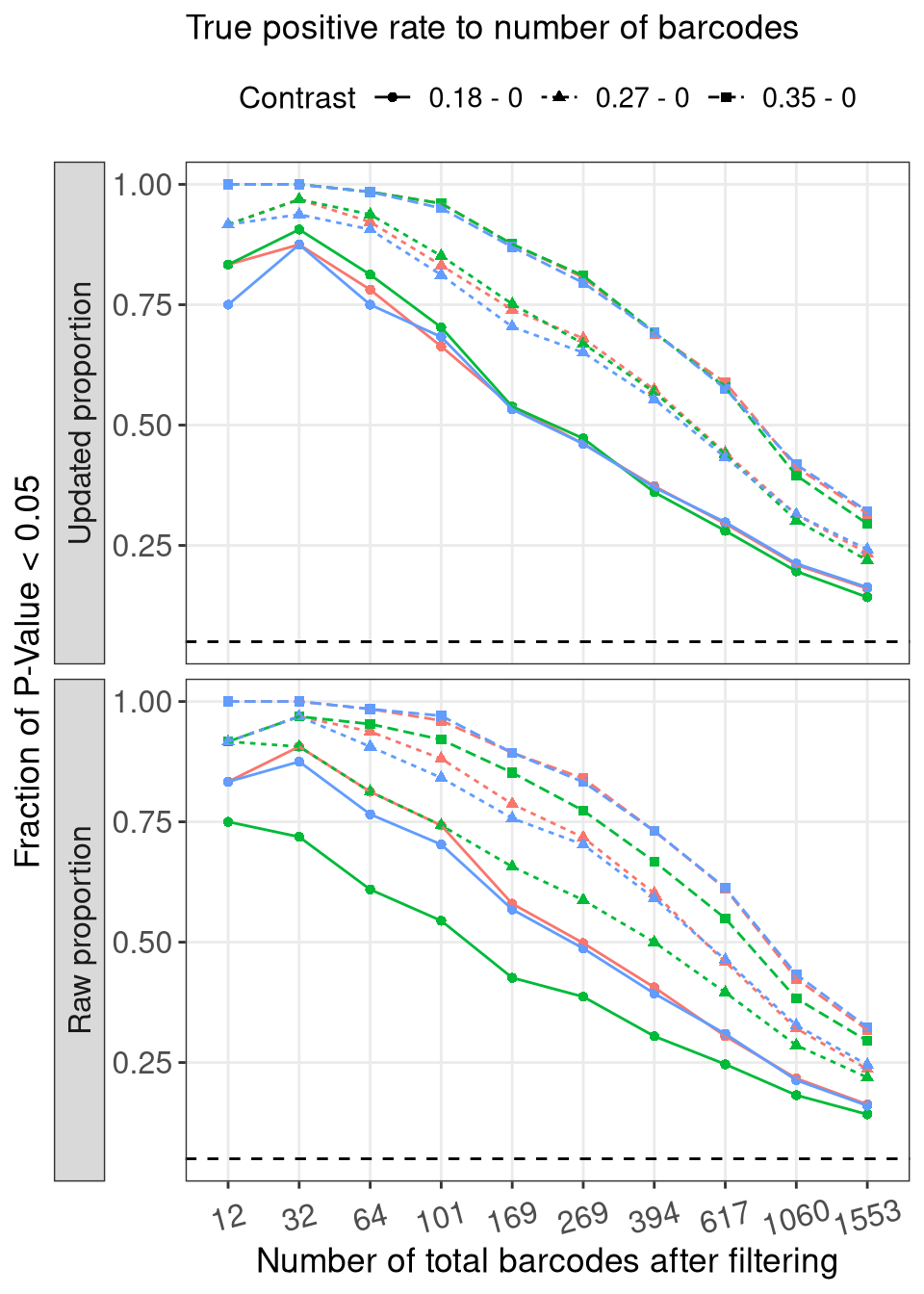

Past versions of unnamed-chunk-37-1.png

Version	Author	Date
34f5894	FeiLiyang	2026-01-01
a2e7a36	FeiLiyang	2025-12-17
dfa737a	FeiLiyang	2025-12-17

8.7 F3F: TPR in quantiles

# plot_tpr_on_quantile(test_all_levels %>% filter(filter_level==0.1), num_quantiles = 4)
# plot_tpr_on_quantile(test_all_levels %>% filter(filter_level==0.2), num_quantiles = 10)
# plot_tpr_on_quantile(test_all_levels %>% filter(filter_level==0.3), num_quantiles = 10)
# plot_tpr_on_quantile(test_all_levels %>% filter(filter_level==0.4), num_quantiles = 10)
# plot_tpr_on_quantile(test_all_levels %>% filter(filter_level==0.5), num_quantiles = 10)
# plot_tpr_on_quantile(test_all_levels %>% filter(filter_level==0.6), num_quantiles = 10)
# plot_tpr_on_quantile(test_all_levels %>% filter(filter_level==0.7), num_quantiles = 10)
# plot_tpr_on_quantile(test_all_levels %>% filter(filter_level==0.8), num_quantiles = 10)
# plot_tpr_on_quantile(test_all_levels %>% filter(filter_level==0.9), num_quantiles = 10)

plot_tpr_on_quantile(test_all_levels %>% filter(filter_level==0.95), num_quantiles = 10) +
  theme_barbieQ() +
  labs(title = "True positive rate in quanties") -> f3f

8.8 FS3B: Residules

resi_none <- lapply(c(0.18, 0.27, 0.35), function(i) get_residules(mixed, mixed_design, myblock, a = i, trans = "none"))
resi_asin <- lapply(c(0.18, 0.27, 0.35), function(i) get_residules(mixed, mixed_design, myblock, a = i, trans = "asin-sqrt"))
resi_logit <- lapply(c(0.18, 0.27, 0.35), function(i) get_residules(mixed, mixed_design, myblock, a = i, trans = "logit"))

resi_df <- rbind(do.call(rbind, resi_none), do.call(rbind, resi_asin), do.call(rbind, resi_logit))

• Distribution and QQ plot.

p_resid_distr_35 <- ggplot(resi_df %>% filter(Contrast == "0.35 - 0"),
                        aes(x = Residual, color = Method)) +
  geom_density() +
  labs(x = "Residual", y = "Density") +
  facet_wrap(~Method, scales = "free", ncol = 1, strip.position = "left") +
  theme_bw() +
  theme(legend.position = "none", plot.title.position = "panel")


p_resid_qq_35 <- ggplot(resi_df %>% filter(Contrast == "0.35 - 0"), 
                     aes(sample = Residual, color = Method)) +
  stat_qq() +
  stat_qq_line(color = "black", linetype = "dashed") +
  labs(x = "Normal Quantiles", y = "\n Residual Quuantiles") +
  facet_wrap(~Method, scales = "free", ncol = 1) +
  theme_bw() +
  theme(legend.position = "none", strip.text = element_blank(), plot.title.position = "panel")

fs3b <- (p_resid_distr_35 + 
  theme(legend.title = element_text(size = 12), legend.text = element_text(size = 11), strip.text = element_text(size = 12),
        axis.title = element_text(size = 13), axis.text = element_text(size = 10))
  ) +
(p_resid_qq_35 + 
  theme(legend.title = element_text(size = 12), legend.text = element_text(size = 11), 
        axis.title = element_text(size = 13), axis.text = element_text(size = 10)))

fs3b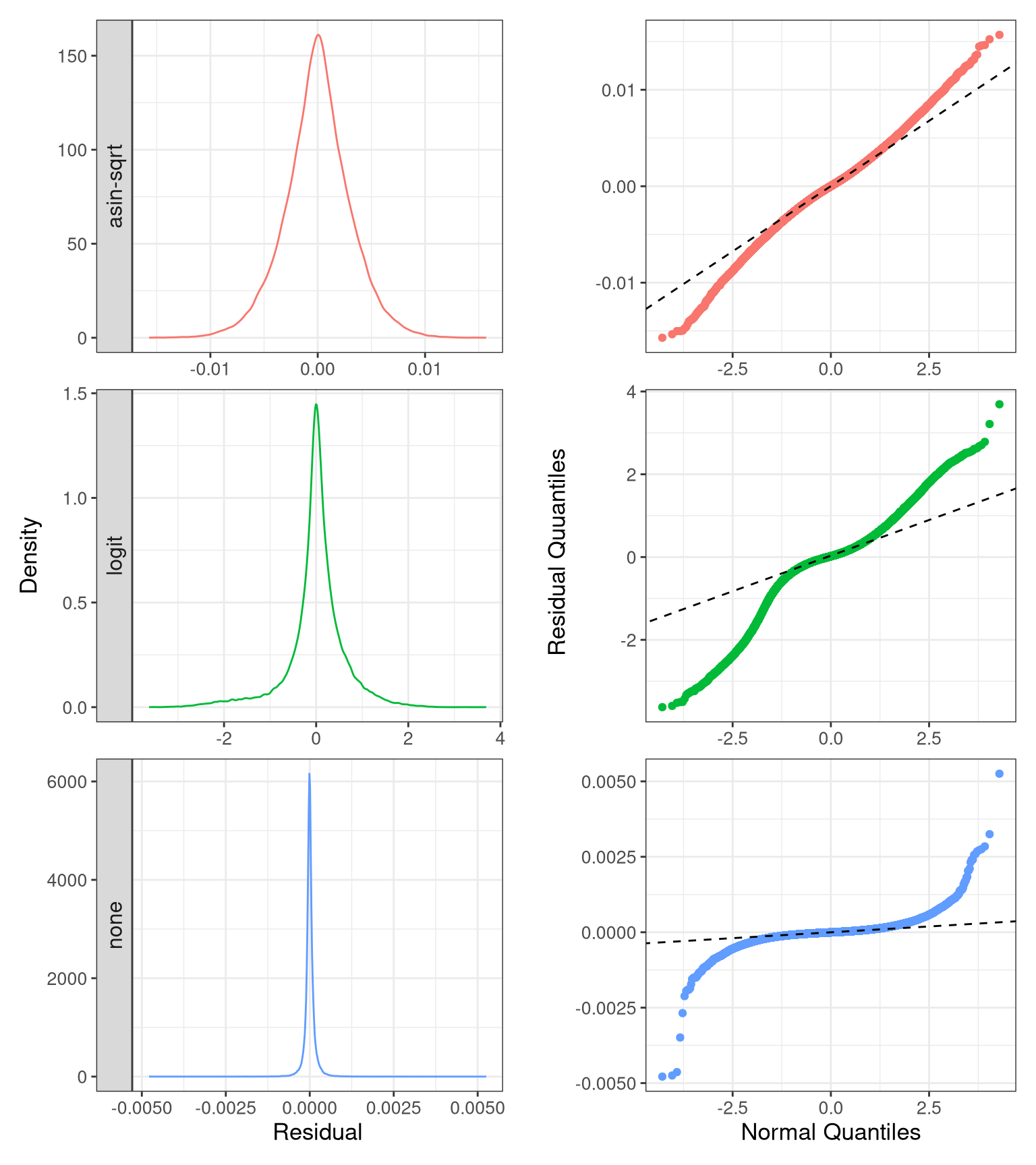

Past versions of unnamed-chunk-41-1.png

Version	Author	Date
34f5894	FeiLiyang	2026-01-01

p_resid_distr_27 <- ggplot(resi_df %>% filter(Contrast == "0.27 - 0"), aes(x = Residual, color = Method)) +
  geom_density() +
  labs(x = "Residual", y = "Density") +
  facet_wrap(~Method, scales = "free", ncol = 1) +
  theme_bw() +
  theme(legend.position = "none", strip.text = element_blank())

p_resid_qq_27 <- ggplot(resi_df %>% filter(Contrast == "0.27 - 0"), aes(sample = Residual, color = Method)) +
  stat_qq() +
  stat_qq_line(color = "black", linetype = "dashed") +
  labs(x = "Normal Quantiles", y = "Residule Quantiles") +
  facet_wrap(~Method, scales = "free", ncol = 1) +
  theme_bw() +
  theme(legend.position = "none", strip.text = element_blank())

p_resid_distr_18 <- ggplot(resi_df %>% filter(Contrast == "0.18 - 0"), aes(x = Residual, color = Method)) +
  geom_density() +
  labs(x = "Residual", y = "Density") +
  facet_wrap(~Method, scales = "free", ncol = 1) +
  theme_bw() +
  theme(legend.position = "none", strip.text = element_blank())

p_resid_qq_18 <- ggplot(resi_df %>% filter(Contrast == "0.18 - 0"), aes(sample = Residual, color = Method)) +
  stat_qq() +
  stat_qq_line(color = "black", linetype = "dashed") +
  labs(x = "Normal Quantiles", y = "Residule Quantiles") +
  facet_wrap(~Method, scales = "free", ncol = 1) +
  theme_bw() +
  theme(legend.position = "none", strip.text = element_blank())

p_resid_distr_35 + p_resid_distr_27 + p_resid_distr_18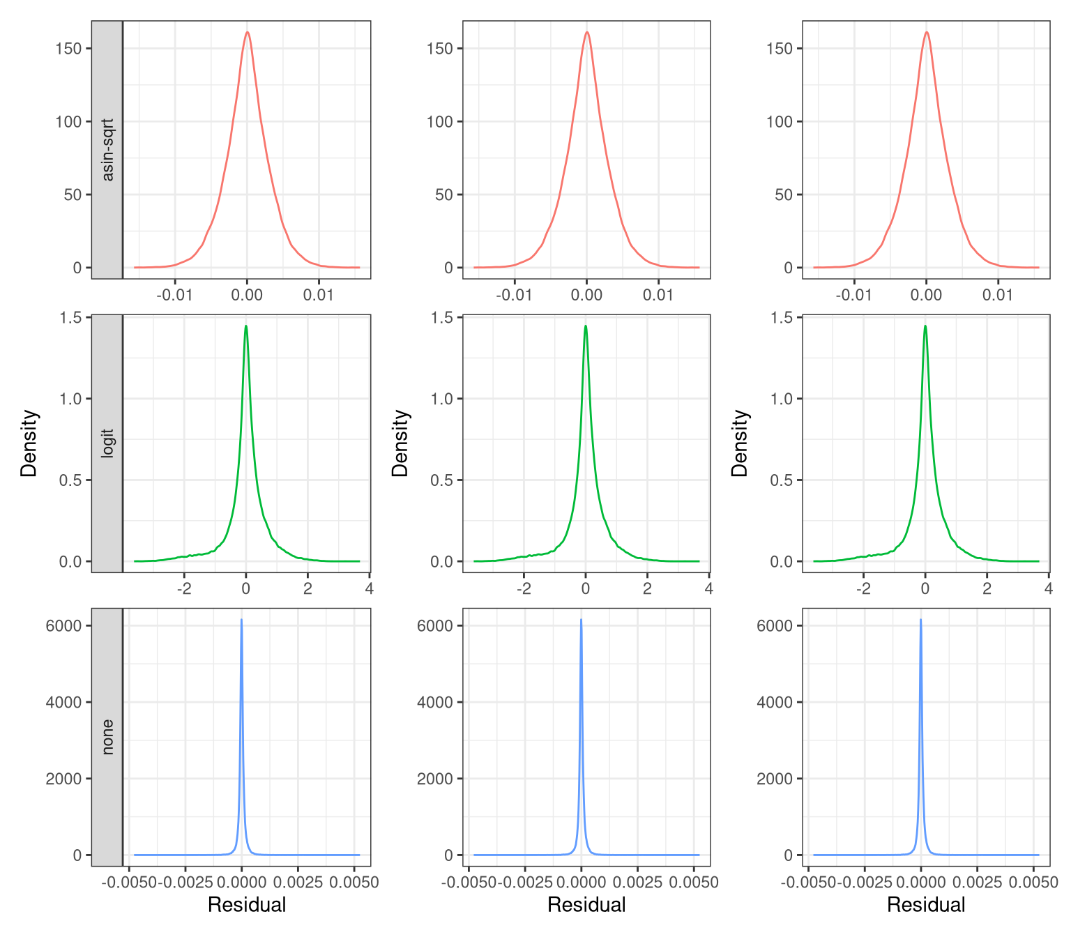

Past versions of unnamed-chunk-43-1.png

Version	Author	Date
34f5894	FeiLiyang	2026-01-01
dfa737a	FeiLiyang	2025-12-17

p_resid_qq_35 + p_resid_qq_27 + p_resid_qq_18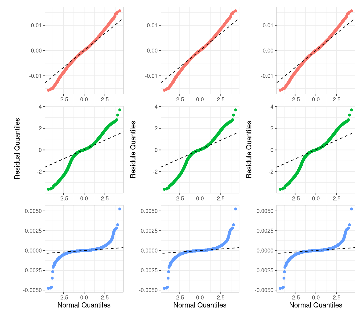

Past versions of unnamed-chunk-43-2.png

Version	Author	Date
34f5894	FeiLiyang	2026-01-01

8.9 Consistency

asin_adjP_3con <- es_de_asin_df %>%
  dplyr::select(BC, Contrast, P.Value) %>%
  tidyr::pivot_wider(
    id_cols = BC,
    names_from = Contrast,
    values_from = P.Value
  )
none_adjP_3con <- es_de_none_df %>%
  dplyr::select(BC, Contrast, P.Value) %>%
  tidyr::pivot_wider(
    id_cols = BC,
    names_from = Contrast,
    values_from = P.Value
  )

eu <- eulerr::euler(list(
  asin_C0.18 = rownames(asin_adjP_3con)[asin_adjP_3con$`0.18 - 0` < 0.05],
  asin_C0.27 = rownames(asin_adjP_3con)[asin_adjP_3con$`0.27 - 0` < 0.05],
  asin_C0.35 = rownames(asin_adjP_3con)[asin_adjP_3con$`0.35 - 0` < 0.05],
  none_C0.18 = rownames(none_adjP_3con)[none_adjP_3con$`0.18 - 0` < 0.05],
  none_C0.27 = rownames(none_adjP_3con)[none_adjP_3con$`0.27 - 0` < 0.05],
  none_C0.35 = rownames(none_adjP_3con)[none_adjP_3con$`0.35 - 0` < 0.05]
))

plot(eu, quantities = TRUE)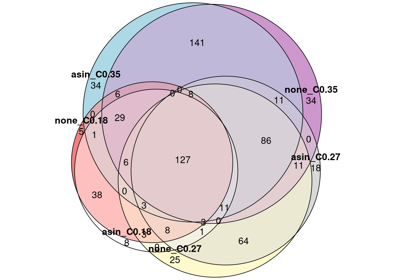

Past versions of unnamed-chunk-45-1.png

Version	Author	Date
34f5894	FeiLiyang	2026-01-01
dfa737a	FeiLiyang	2025-12-17

9 Figure 3

layout = "
AAAAAAAAAAAAA##
AAAAAAAAAAAAA##
AAAAAAAAAAAAA##
BBBBBBBCCCCCCCC
BBBBBBBCCCCCCCC
BBBBBBBCCCCCCCC
BBBBBBBCCCCCCCC
DDDDEEEEEFFFFFF
DDDDEEEEEFFFFFF
DDDDEEEEEFFFFFF
DDDDEEEEEFFFFFF
DDDDEEEEEFFFFFF
GGGGHHHHHIIIIII
GGGGHHHHHIIIIII
GGGGHHHHHIIIIII
GGGGHHHHHIIIIII
GGGGHHHHHIIIIII
GGGGHHHHHIIIIII
GGGGHHHHHIIIIII
"
f3 <- ((wrap_elements(full = f3a) + theme(plot.margin = unit(c(0,0,0,0), "cm"))) + 
    wrap_elements(f3b + theme(plot.margin = unit(rep(0,4), "cm"))) + 
    wrap_elements(f3c + theme(plot.margin = unit(c(0,0,0,0), "cm"))) +
    wrap_elements(f3d + theme(legend.position = "top", plot.margin = unit(rep(0,4), "cm"))) +
    wrap_elements(f3e + theme(legend.position = "top", plot.margin = unit(rep(0,4), "cm"))) +
    wrap_elements(f3f + theme(legend.position = "top", plot.margin = unit(rep(0,4), "cm")) + guides(color = "none")) +
    wrap_elements(f3g + theme(legend.position = "top", plot.margin = unit(c(0,0,0,0), "cm"))) +
    wrap_elements(f3h + theme(legend.position = "top",plot.margin = unit(rep(0,4), "cm"))) +
    wrap_elements(f3i + theme(legend.position = "top",plot.margin = unit(rep(0,4), "cm"))) 
      
    )+ 
  plot_layout(design = layout) +
  ## space is okay but must be unique
  plot_annotation(tag_levels = list(c("A", "B","C", "D", "E", "F", "G", "H", "I"))) &
  theme(plot.tag = element_text(size = 24, face = "bold", family = "arial"))

f3

Ignoring unknown labels:
• titlte : ""

Warning: No shared levels found between `names(values)` of the manual scale and the
data's colour values.

Ignoring unknown labels:
• shape : "N_sample"
• linetype : "N_sample"
Ignoring unknown labels:
• shape : "N_sample"
• linetype : "N_sample"

Warning: Removed 165 rows containing non-finite outside the scale range
(`stat_boxplot()`).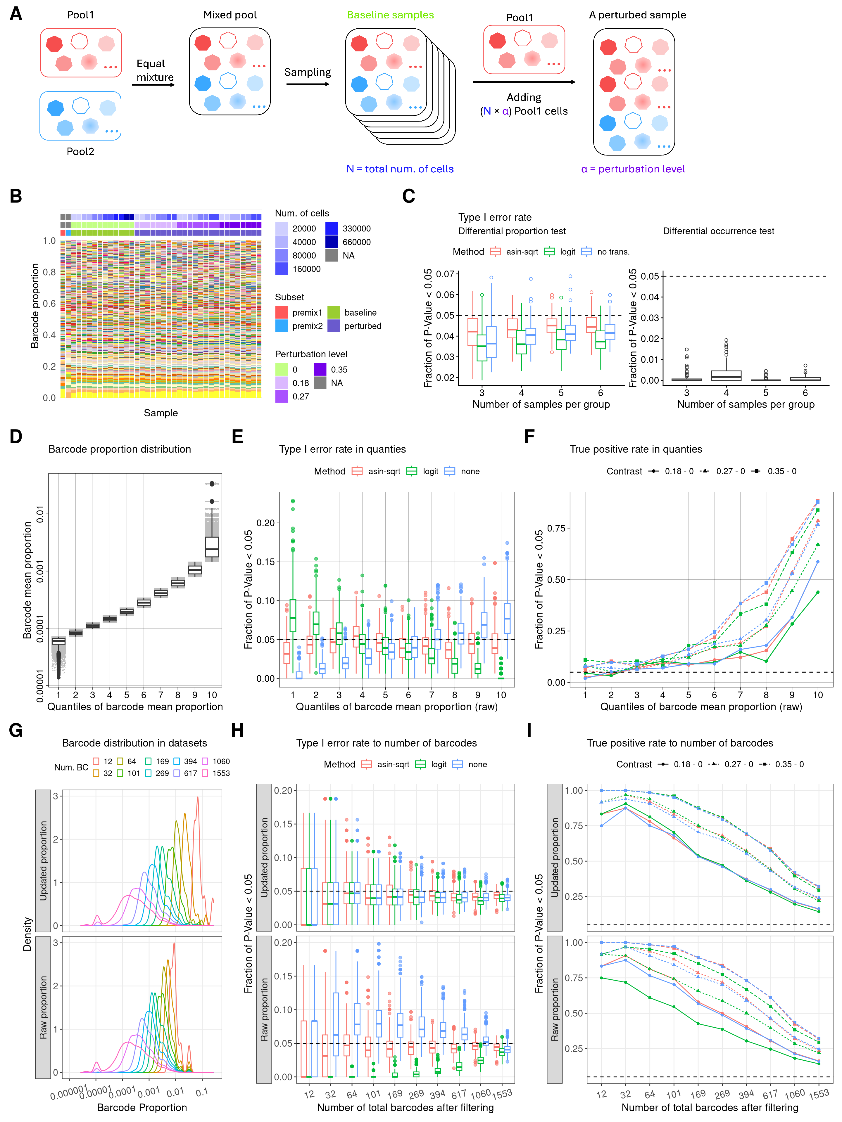

Past versions of unnamed-chunk-46-1.png

Version	Author	Date
34f5894	FeiLiyang	2026-01-01
a2e7a36	FeiLiyang	2025-12-17

ggsave(
  filename = "output/f3.png",
  plot = f3,
  width = 15,
  height = 20,
  units = "in", # for Rmd r chunk fig size, unit default to inch
  dpi = 350
  )

Ignoring unknown labels:
• titlte : ""

Warning: No shared levels found between `names(values)` of the manual scale and the
data's colour values.

Ignoring unknown labels:
• shape : "N_sample"
• linetype : "N_sample"
Ignoring unknown labels:
• shape : "N_sample"
• linetype : "N_sample"

Warning: Removed 165 rows containing non-finite outside the scale range
(`stat_boxplot()`).

Saving this figure in f3

10 Figure S3

layoutS4 = "
AAABB
AAABB
AAABB
"
fs3 <- (
    wrap_elements(fs3a + theme(plot.margin = unit(rep(0,4), "cm"))) + 
    wrap_elements(fs3b + theme(plot.margin = unit(c(0,0,0,0), "cm")))
    )+ 
  plot_layout(design = layoutS4) +
  ## space is okay but must be unique
  plot_annotation(tag_levels = list(c("A", "B"))) &
  theme(plot.tag = element_text(size = 24, face = "bold", family = "arial"))

fs3

Warning: Removed 7 rows containing missing values or values outside the scale range
(`geom_point()`).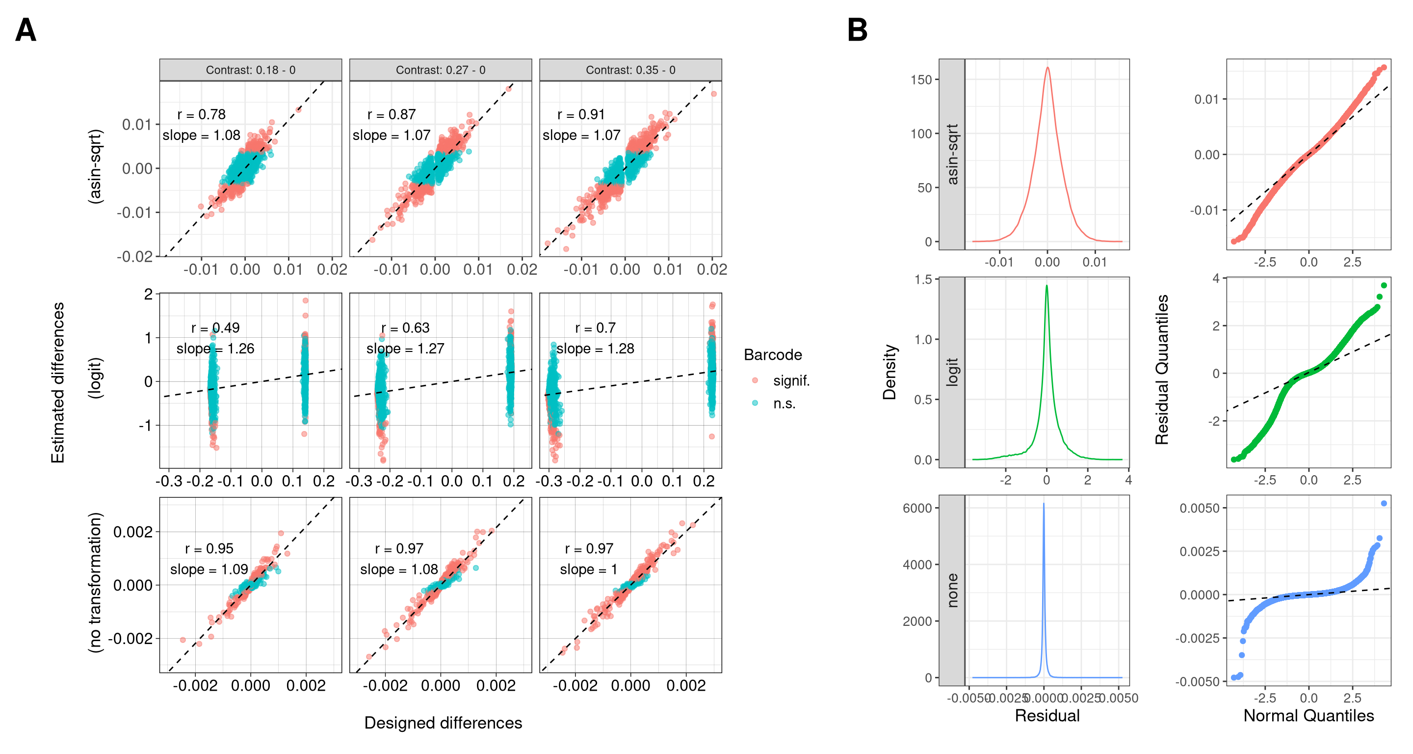

Past versions of unnamed-chunk-48-1.png

Version	Author	Date
34f5894	FeiLiyang	2026-01-01
dfa737a	FeiLiyang	2025-12-17

ggsave(
  filename = "output/fs3.png",
  plot = fs3,
  width = 15,
  height = 8,
  units = "in", # for Rmd r chunk fig size, unit default to inch
  dpi = 350
  )

Warning: Removed 7 rows containing missing values or values outside the scale range
(`geom_point()`).

Saving this figure in fs3

Session information

sessionInfo()

R version 4.5.0 (2025-04-11)
Platform: x86_64-pc-linux-gnu
Running under: Red Hat Enterprise Linux 9.6 (Plow)

Matrix products: default
BLAS/LAPACK: FlexiBLAS OPENBLAS-OPENMP;  LAPACK version 3.9.0

locale:
 [1] LC_CTYPE=en_AU.UTF-8       LC_NUMERIC=C              
 [3] LC_TIME=en_AU.UTF-8        LC_COLLATE=en_AU.UTF-8    
 [5] LC_MONETARY=en_AU.UTF-8    LC_MESSAGES=en_AU.UTF-8   
 [7] LC_PAPER=en_AU.UTF-8       LC_NAME=C                 
 [9] LC_ADDRESS=C               LC_TELEPHONE=C            
[11] LC_MEASUREMENT=en_AU.UTF-8 LC_IDENTIFICATION=C       

time zone: Australia/Melbourne
tzcode source: system (glibc)

attached base packages:
[1] grid      stats4    stats     graphics  grDevices utils     datasets 
[8] methods   base     

other attached packages:
 [1] barbieQ_1.1.3               edgeR_4.6.3                
 [3] limma_3.64.3                eulerr_7.0.4               
 [5] magick_2.9.0                ComplexHeatmap_2.24.1      
 [7] ggVennDiagram_1.5.4         scales_1.4.0               
 [9] patchwork_1.3.2             ggnewscale_0.5.2           
[11] ggbreak_0.1.6               ggplot2_4.0.0              
[13] SummarizedExperiment_1.38.1 Biobase_2.68.0             
[15] GenomicRanges_1.60.0        GenomeInfoDb_1.44.3        
[17] IRanges_2.42.0              S4Vectors_0.48.0           
[19] BiocGenerics_0.54.0         generics_0.1.4             
[21] MatrixGenerics_1.20.0       matrixStats_1.5.0          
[23] data.table_1.17.8           knitr_1.50                 
[25] tibble_3.3.0                tidyr_1.3.1                
[27] dplyr_1.1.4                 magrittr_2.0.4             
[29] readxl_1.4.5                workflowr_1.7.2            

loaded via a namespace (and not attached):
  [1] RColorBrewer_1.1-3      rstudioapi_0.17.1       jsonlite_2.0.0         
  [4] shape_1.4.6.1           jomo_2.7-6              nloptr_2.2.1           
  [7] farver_2.1.2            logistf_1.26.1          rmarkdown_2.30         
 [10] ragg_1.5.0              GlobalOptions_0.1.2     fs_1.6.6               
 [13] vctrs_0.6.5             minqa_1.2.8             memoise_2.0.1          
 [16] htmltools_0.5.8.1       S4Arrays_1.8.1          broom_1.0.10           
 [19] cellranger_1.1.0        SparseArray_1.8.1       gridGraphics_0.5-1     
 [22] mitml_0.4-5             sass_0.4.10             bslib_0.9.0            
 [25] cachem_1.1.0            whisker_0.4.1           igraph_2.1.4           
 [28] lifecycle_1.0.4         iterators_1.0.14        pkgconfig_2.0.3        
 [31] Matrix_1.7-3            R6_2.6.1                fastmap_1.2.0          
 [34] rbibutils_2.3           GenomeInfoDbData_1.2.14 clue_0.3-66            
 [37] digest_0.6.37           aplot_0.2.9             colorspace_2.1-2       
 [40] ps_1.9.1                rprojroot_2.1.1         textshaping_1.0.3      
 [43] labeling_0.4.3          httr_1.4.7              polyclip_1.10-7        
 [46] abind_1.4-8             mgcv_1.9-1              compiler_4.5.0         
 [49] withr_3.0.2             doParallel_1.0.17       backports_1.5.0        
 [52] S7_0.2.0                viridis_0.6.5           ggforce_0.5.0          
 [55] pan_1.9                 MASS_7.3-65             rappdirs_0.3.3         
 [58] DelayedArray_0.34.1     rjson_0.2.23            tools_4.5.0            
 [61] httpuv_1.6.16           nnet_7.3-20             glue_1.8.0             
 [64] callr_3.7.6             nlme_3.1-168            promises_1.3.3         
 [67] polylabelr_0.3.0        getPass_0.2-4           cluster_2.1.8.1        
 [70] operator.tools_1.6.3    gtable_0.3.6            formula.tools_1.7.1    
 [73] tidygraph_1.3.1         XVector_0.48.0          ggrepel_0.9.6          
 [76] foreach_1.5.2           pillar_1.11.1           stringr_1.5.2          
 [79] yulab.utils_0.2.1       later_1.4.4             circlize_0.4.16        
 [82] splines_4.5.0           tweenr_2.0.3            lattice_0.22-6         
 [85] survival_3.8-3          tidyselect_1.2.1        locfit_1.5-9.12        
 [88] git2r_0.36.2            reformulas_0.4.1        gridExtra_2.3          
 [91] xfun_0.53               graphlayouts_1.2.2      statmod_1.5.0          
 [94] stringi_1.8.7           UCSC.utils_1.4.0        boot_1.3-31            
 [97] ggfun_0.2.0             yaml_2.3.10             evaluate_1.0.5         
[100] codetools_0.2-20        ggraph_2.2.2            ggplotify_0.1.3        
[103] cli_3.6.5               rpart_4.1.24            systemfonts_1.3.1      
[106] Rdpack_2.6.4            processx_3.8.6          jquerylib_0.1.4        
[109] Rcpp_1.1.0              png_0.1-8               parallel_4.5.0         
[112] lme4_1.1-37             glmnet_4.1-10           viridisLite_0.4.2      
[115] purrr_1.1.0             crayon_1.5.3            GetoptLong_1.0.5       
[118] rlang_1.1.6             mice_3.18.0