Last updated: 2026-01-11

Checks: 5 2

Knit directory: public_barcode_count/

This reproducible R Markdown analysis was created with workflowr (version 1.7.2). The Checks tab describes the reproducibility checks that were applied when the results were created. The Past versions tab lists the development history.

R Markdown file: uncommitted changes

The R Markdown file has unstaged changes. To know which version of the R Markdown file created these results, you’ll want to first commit it to the Git repo. If you’re still working on the analysis, you can ignore this warning. When you’re finished, you can run wflow_publish to commit the R Markdown file and build the HTML.

Environment: objects present

The global environment had objects present when the code in the R Markdown file was run. These objects can affect the analysis in your R Markdown file in unknown ways. For reproduciblity it’s best to always run the code in an empty environment. Use wflow_publish or wflow_build to ensure that the code is always run in an empty environment.

The following objects were defined in the global environment when these results were created:

Name	Class	Size
module	function	5.6 Kb

Seed: set.seed(20250112)

The command set.seed(20250112) was run prior to running the code in the R Markdown file. Setting a seed ensures that any results that rely on randomness, e.g. subsampling or permutations, are reproducible.

Session information: recorded

Great job! Recording the operating system, R version, and package versions is critical for reproducibility.

Cache: none

Nice! There were no cached chunks for this analysis, so you can be confident that you successfully produced the results during this run.

File paths: relative

Great job! Using relative paths to the files within your workflowr project makes it easier to run your code on other machines.

Repository version: 506c314

Great! You are using Git for version control. Tracking code development and connecting the code version to the results is critical for reproducibility.

The results in this page were generated with repository version 506c314. See the Past versions tab to see a history of the changes made to the R Markdown and HTML files.

Note that you need to be careful to ensure that all relevant files for the analysis have been committed to Git prior to generating the results (you can use wflow_publish or wflow_git_commit). workflowr only checks the R Markdown file, but you know if there are other scripts or data files that it depends on. Below is the status of the Git repository when the results were generated:


Ignored files:
    Ignored:    .RData
    Ignored:    .Rhistory
    Ignored:    .Rproj.user/
    Ignored:    public_barcode_count.Rproj

Unstaged changes:
    Modified:   analysis/barbieQ_paper_Figure4.Rmd

Note that any generated files, e.g. HTML, png, CSS, etc., are not included in this status report because it is ok for generated content to have uncommitted changes.

These are the previous versions of the repository in which changes were made to the R Markdown (analysis/barbieQ_paper_Figure4.Rmd) and HTML (docs/barbieQ_paper_Figure4.html) files. If you’ve configured a remote Git repository (see ?wflow_git_remote), click on the hyperlinks in the table below to view the files as they were in that past version.

File	Version	Author	Date	Message
Rmd	f48add2	FeiLiyang	2026-01-07	supple analyses
Rmd	34f5894	FeiLiyang	2026-01-01	reorder f3
Rmd	7b7813d	FeiLiyang	2025-12-17	update f3 fs4
html	7b7813d	FeiLiyang	2025-12-17	update f3 fs4
Rmd	c2766f9	Liyang Fei	2025-10-07	remake figures

1 Load Dependencies

library(readxl)
library(magrittr)
library(dplyr)
library(tidyr) # for pivot_longer
library(tibble) # for rownames_to _column
library(knitr) # for kable()
library(data.table) # for data.table()
library(SummarizedExperiment)
library(S4Vectors)
library(grid)
library(ggplot2)
library(ggbreak)
library(ggnewscale) # ggnewscale::new_scale_fill() 
library(patchwork)
library(scales)
library(ggVennDiagram)
library(ComplexHeatmap)
library(magick)
library(eulerr)
library(edgeR)

source("analysis/plotBarcodeHistogram.R") ## accommodated from bartools::plotBarcodehistogram
source("analysis/F4_validation.R") ## functions for Figure4 validations
source("analysis/ggplot_theme.R") ## setting ggplot theme

2 Install `barbieQ`

Installing the latest devel version of barbieQ from GitHub.

if (!requireNamespace("barbieQ", quietly = TRUE)) {
  remotes::install_github("Oshlack/barbieQ")
}

Warning: replacing previous import 'data.table::first' by 'dplyr::first' when
loading 'barbieQ'

Warning: replacing previous import 'data.table::last' by 'dplyr::last' when
loading 'barbieQ'

Warning: replacing previous import 'data.table::between' by 'dplyr::between'
when loading 'barbieQ'

Warning: replacing previous import 'dplyr::as_data_frame' by
'igraph::as_data_frame' when loading 'barbieQ'

Warning: replacing previous import 'dplyr::groups' by 'igraph::groups' when
loading 'barbieQ'

Warning: replacing previous import 'dplyr::union' by 'igraph::union' when
loading 'barbieQ'

library(barbieQ)

Check the version of barbieQ.

packageVersion("barbieQ")

[1] '1.1.3'

3 Set seeds

set.seed(2025)

4 Load preprocessed data

Loading barbieQ object preprocessed from barbieQ_paper_Figure2

load("output/monkeyHSPC_barbieQ.rda")
# load("output/monkeyHSPC_raw_barbieQ.rda")

5 F4A: Experimental schematic

schematic <- image_read("output/f4a_schematic.jpeg")
f4a <- rasterGrob(schematic, interpolate = FALSE) 
wrap_elements(full = f4a)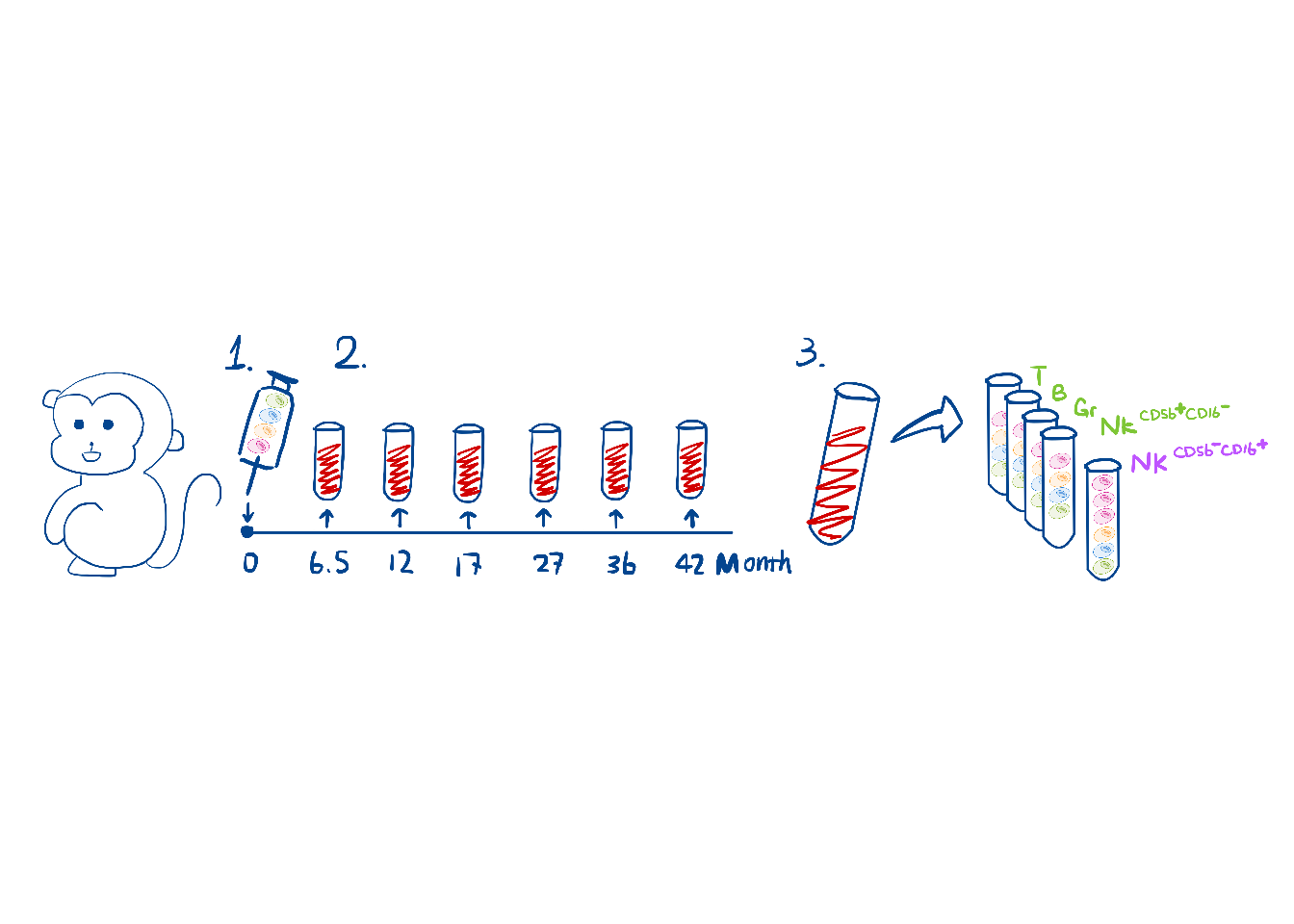

Version	Author	Date
dfa737a	FeiLiyang	2025-12-17

6 F4B: Plot barcode proportion and sample annotation

plotBarcodeHistogram is customized from the bartools package.

## get sample conditions and color mapping
metadata <- monkeyHSPC_merged_top$sampleMetadata %>% as.data.frame()
metadata$sample <- rownames(metadata)
metadata$y = 1.05 ## for ggplot tile position
color_mapping <- monkeyHSPC_merged_top@metadata$factorColors

## order samples
order_sample <- metadata %>% with(order(Celltype, Months))

monkey_dge <- DGEList(
  counts = assay(monkeyHSPC_merged_top), 
  group = metadata$Celltype)

## pull out ggplot data
p_stacked_prop <- plotBarcodeHistogram(monkey_dge, orderSamples = colnames(monkeyHSPC_merged_top)[order_sample])

Warning: Use of .data in tidyselect expressions was deprecated in tidyselect 1.2.0.
ℹ Please use `"barcode"` instead of `.data$barcode`
This warning is displayed once every 8 hours.
Call `lifecycle::last_lifecycle_warnings()` to see where this warning was
generated.

Warning: Use of .data in tidyselect expressions was deprecated in tidyselect 1.2.0.
ℹ Please use `"value"` instead of `.data$value`
This warning is displayed once every 8 hours.
Call `lifecycle::last_lifecycle_warnings()` to see where this warning was
generated.

Warning: Use of .data in tidyselect expressions was deprecated in tidyselect 1.2.0.
ℹ Please use `"name"` instead of `.data$name`
This warning is displayed once every 8 hours.
Call `lifecycle::last_lifecycle_warnings()` to see where this warning was
generated.

Warning: Use of .data in tidyselect expressions was deprecated in tidyselect 1.2.0.
ℹ Please use `"freq"` instead of `.data$freq`
This warning is displayed once every 8 hours.
Call `lifecycle::last_lifecycle_warnings()` to see where this warning was
generated.

f4b <- p_stacked_prop +
  ## label perturbations
  ggnewscale::new_scale_fill() +
  geom_tile(data = metadata, aes(x = sample,y = y, fill = Celltype), height = 0.04, inherit.aes = FALSE, color = "white") +
  scale_fill_manual(values = color_mapping$Celltype) +
  labs(fill = "Cell type") + 
  ## label libsize
  ggnewscale::new_scale_fill() +
  geom_tile(data = metadata, aes(x = sample,y = y+0.05, fill = as.factor(Months)), height = 0.04, inherit.aes = FALSE, color = "white") +
  scale_fill_manual(values = setNames(attr(color_mapping$Months, "colors"), attr(color_mapping$Months, "breaks"))) +
  labs(fill = "Month") +
  labs(x = "Sample", y = "Barcode proportion") +
  theme_minimal() +
  scale_y_continuous(breaks = seq(0, 1, by = 0.2)) +
  theme(axis.text.x = element_blank(), panel.grid.major.x = element_blank())

f4b

Warning: The `guide` argument in `scale_*()` cannot be `FALSE`. This was deprecated in
ggplot2 3.3.4.
ℹ Please use "none" instead.
This warning is displayed once every 8 hours.
Call `lifecycle::last_lifecycle_warnings()` to see where this warning was
generated.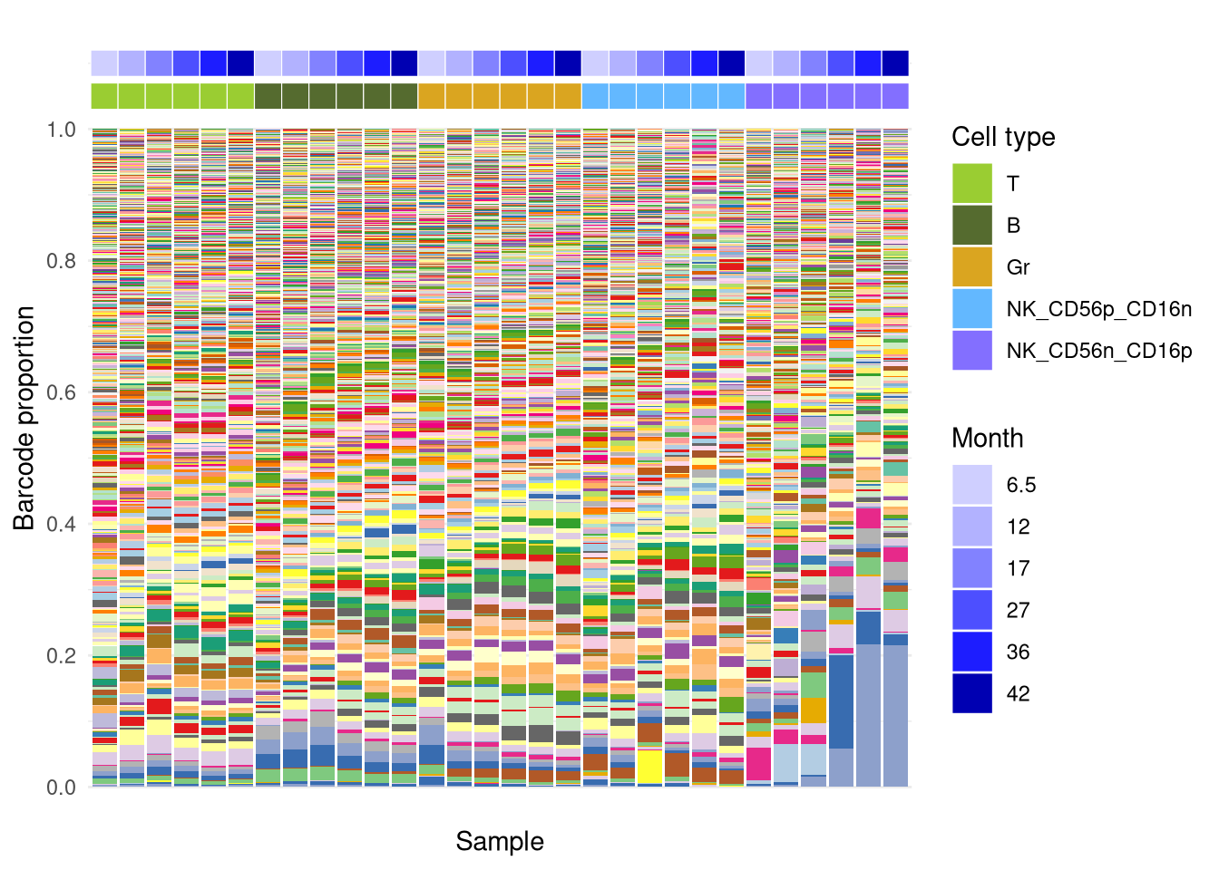

Version	Author	Date
dfa737a	FeiLiyang	2025-12-17

7 Compare filtering

7.1 F4D: top10each vs. barbieQ filter

The original paper filter barcodes by tagging top 10 barcodes from each sample, and collectively keeping the tagged barcodes across all samples. Here we compare this “top10each” (and “top20each”) strategy with barbieQ filtering.

The tagTopN function is sourced from “F4_validation.R”.

## tagging top 10 in all samples
colTags <- lapply(as.data.frame(assays(monkeyHSPC_merged)$proportion), function(col) tagTopN(col, N = 10))
colTagMat <- do.call(cbind, colTags) %>% as.matrix()
colnames(colTagMat) <- colnames(monkeyHSPC_merged)
rownames(colTagMat) <- rownames(monkeyHSPC_merged)
## filtering by keeping barcodes tagged for at least once
colTagVec <- rowSums(colTagMat) >= 1
## ensuring we've tagged 10 barcodes within each sample
all(colSums(colTagMat) == 10)

[1] TRUE

## copying the barbieQ object and manually labeling the filtered barcodes based on the above strategy
monkeyHSPC_top10each <- monkeyHSPC_merged
rowData(monkeyHSPC_top10each)$isTopBarcode$isTop <- colTagVec
assays(monkeyHSPC_top10each)$isTopAssay <- colTagMat
p_sankey_top10 <- barbieQ::plotBarcodeSankey(monkeyHSPC_top10each)
p_sankey_barbieQ <- barbieQ::plotBarcodeSankey(monkeyHSPC_merged)

## repeat the process for top20 each
colTags2 <- lapply(as.data.frame(assays(monkeyHSPC_merged)$proportion), function(col) tagTopN(col, N = 20))
colTagMat2 <- do.call(cbind, colTags2) %>% as.matrix()
colnames(colTagMat2) <- colnames(monkeyHSPC_merged)
rownames(colTagMat2) <- rownames(monkeyHSPC_merged)
colTagVec2 <- rowSums(colTagMat2) >= 1
all(colSums(colTagMat2) == 20)

[1] TRUE

monkeyHSPC_top20each <- monkeyHSPC_merged
rowData(monkeyHSPC_top20each)$isTopBarcode$isTop <- colTagVec2
assays(monkeyHSPC_top20each)$isTopAssay <- colTagMat2
p_sankey_top20 <- barbieQ::plotBarcodeSankey(monkeyHSPC_top20each)


## plot sankeys
f4d <- p_sankey_barbieQ + 
  theme(legend.position = "none", plot.title = element_text(hjust = 0.5, vjust = 1), 
        strip.text.x = element_blank(), strip.text.y = element_blank()) + labs(title = "barbieQ") +
  p_sankey_top10 + 
  theme(legend.position = "none", plot.title = element_text(hjust = 0.5, vjust = 1),
        strip.text.x = element_blank(), strip.text.y = element_blank()) + labs(title = "top10each") + 
  p_sankey_top20 + 
  theme(legend.position = "right", plot.title = element_text(hjust = 0.5, vjust = 1),
        strip.text.x = element_blank(), strip.text.y = element_blank()) + labs(title = "top20each")

f4d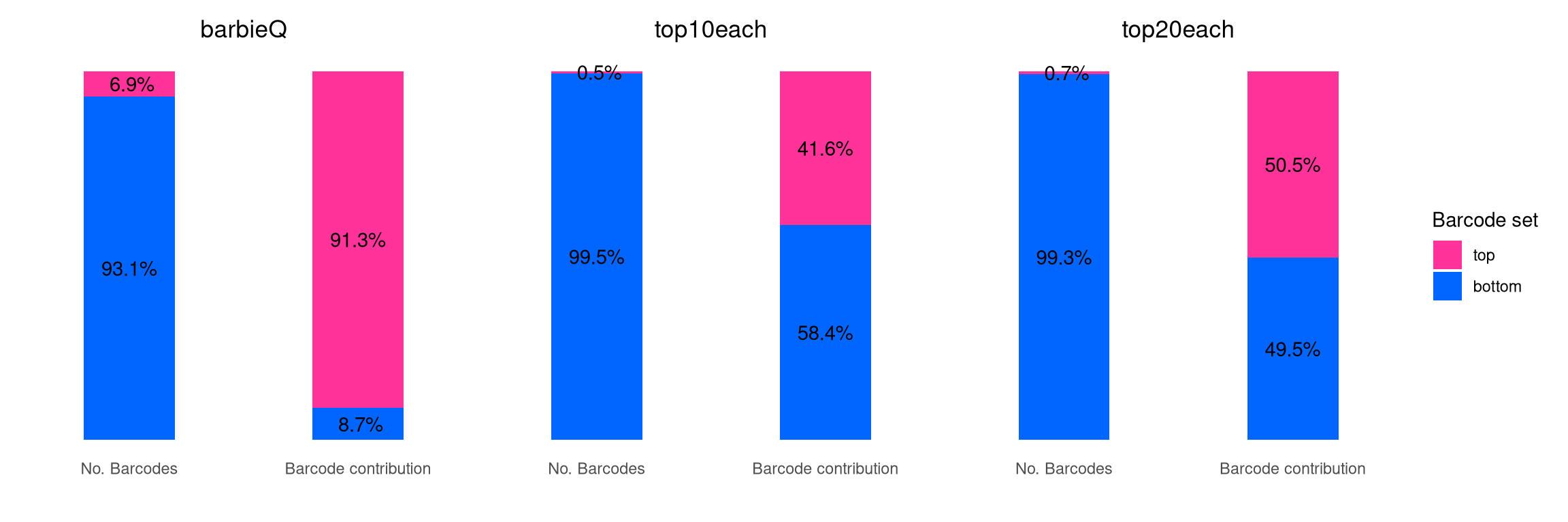

Version	Author	Date
dfa737a	FeiLiyang	2025-12-17

7.2 F4C: overlap

list_top_BC <- list(
  barbieQ = rownames(monkeyHSPC_merged)[monkeyHSPC_merged@elementMetadata$isTopBarcode$isTop],
  top10each = rownames(monkeyHSPC_merged)[colTagVec],
  top20each = rownames(monkeyHSPC_merged)[colTagVec2]
  )

## plot Euler
# venn_filter <- eulerr::euler(list_top_BC) %>% 
#   plot(fills = c("pink", "skyblue", "steelblue"), 
#        alpha = 0.5, labels = list(font = 4, cex = 1), quantities = list(font = 1, cex = 1)) 
# 
# venn_filter %>% plot() %>% grid.grabExpr() %>% wrap_plots()

## plot ggVenn
# ggVennDiagram(list_top_BC, label = "count") + scale_fill_gradient(low="white", high = "skyblue")

## plot UpSet plot
f4c <- list_top_BC %>% 
  Venn() %>% 
  plot_upset(top.bar.numbers.size = 4, relative_width = 0.0) ## limit space for left bar plot

## getting theme settings from an example ggplot using barbieQ theme
tester <- ggplot(data.frame(X = 1:3, Y = 4:6)) +
  geom_point(aes(x = X, y = Y)) +
  theme_barbieQ_size()

tester_col <- ggplot(data.frame(X = 1:3, Y = 4:6)) +
  geom_col(aes(x = X, y = Y), width = 0.2)
tester_col@layers$geom_col$aes_params$width

[1] 0.2

mytittle <- tester@theme$axis.title
mytext <- tester@theme$axis.text

## modifying components in UpSet plots: three gplot objects
f4c[["plotlist"]][[1]]@theme$axis.title <- mytittle
f4c[["plotlist"]][[1]]@theme$axis.text <- mytext

f4c[["plotlist"]][[2]]@theme$axis.title <- mytittle
f4c[["plotlist"]][[2]]@theme$axis.text <- mytext

f4c[["plotlist"]][[2]]@layers$geom_col$aes_params$width <- 0.4

f4c[["plotlist"]][[3]]@theme$axis.title <- mytittle
f4c[["plotlist"]][[3]]@theme$axis.text <- mytext

f4c[["plotlist"]][[3]]@theme$axis.text@size <- 11
f4c[["plotlist"]][[3]]@theme$axis.text@angle <- 15

## removing the left bar plot
f4c[["plotlist"]][[3]] <- f4c[["plotlist"]][[3]] + theme(
    panel.grid = element_blank(),
    axis.text = element_blank(),
    axis.title = element_blank(),
    axis.ticks = element_blank()
  )

## plot 4c
f4c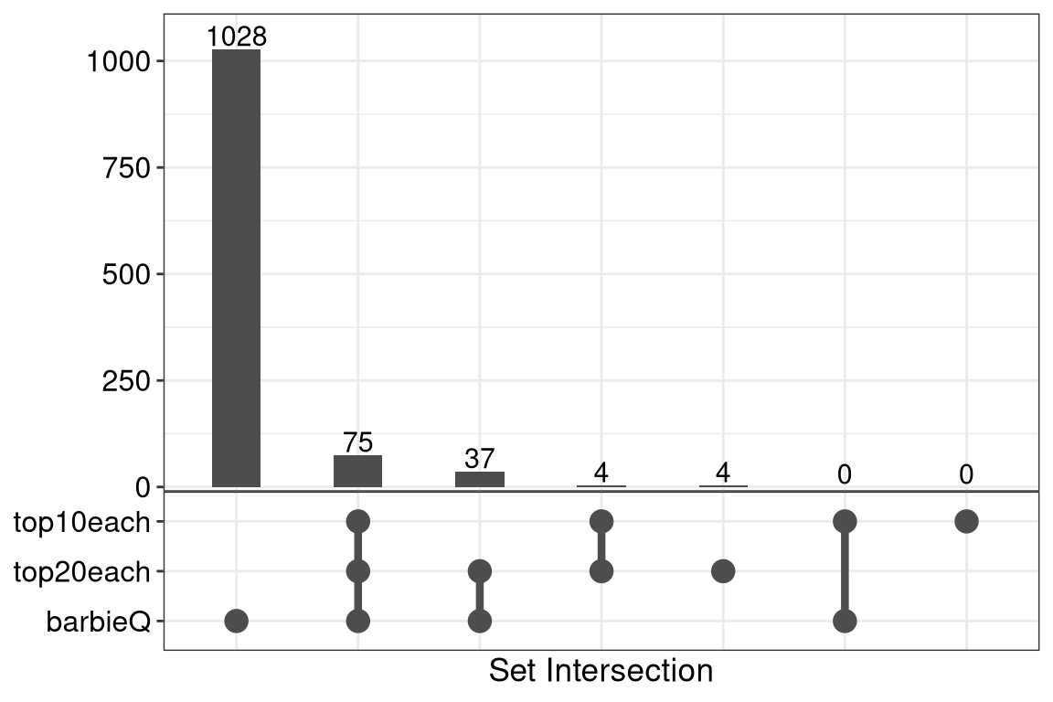

Version	Author	Date
dfa737a	FeiLiyang	2025-12-17

7.3 F4E: inspect two sets: heatmap

barcodeArray <- monkeyHSPC_merged@elementMetadata$isTopBarcode$isTop | colTagVec
length(colTagVec)

[1] 16598

length(monkeyHSPC_merged@elementMetadata$isTopBarcode$isTop)

[1] 16598

table(barcodeArray)

barcodeArray
FALSE  TRUE 
15454  1144

monkeyHSPC_compare_filter <- monkeyHSPC_merged[barcodeArray,]

# Create a named vector indicating where each element belongs
region_labels <- data.frame(
  barcode = rownames(monkeyHSPC_compare_filter),
  region = "both")
region_labels[monkeyHSPC_merged@elementMetadata$isTopBarcode$isTop[barcodeArray] & !(colTagVec[barcodeArray]), "region"] <- "barbieQ only"
region_labels[!(monkeyHSPC_merged@elementMetadata$isTopBarcode$isTop[barcodeArray]) & colTagVec[barcodeArray], "region"] <- "top10each only"

region_labels$region %>% table()

.
  barbieQ only           both top10each only 
          1065             75              4

ht_filter <- plotBarcodeHeatmap(
  monkeyHSPC_compare_filter, 
  barcodeAnnotation = rowAnnotation(
    filteredBy = region_labels$region,
    col = list(filteredBy = c("barbieQ only" = "hotpink", "both" = "slateblue", "top10each only" = "steelblue1")),
    annotation_name_side = "top", annotation_name_rot = 45, annotation_name_gp = grid::gpar(fontsize = 10)))

setting Celltype as the primary factor in `sampleMetadata`.

The automatically generated colors map from the 1^st and 99^th of the
values in the matrix. There are outliers in the matrix whose patterns
might be hidden by this color mapping. You can manually set the color
to `col` argument.

Use `suppressMessages()` to turn off this message.
The automatically generated colors map from the 1^st and 99^th of the
values in the matrix. There are outliers in the matrix whose patterns
might be hidden by this color mapping. You can manually set the color
to `col` argument.

Use `suppressMessages()` to turn off this message.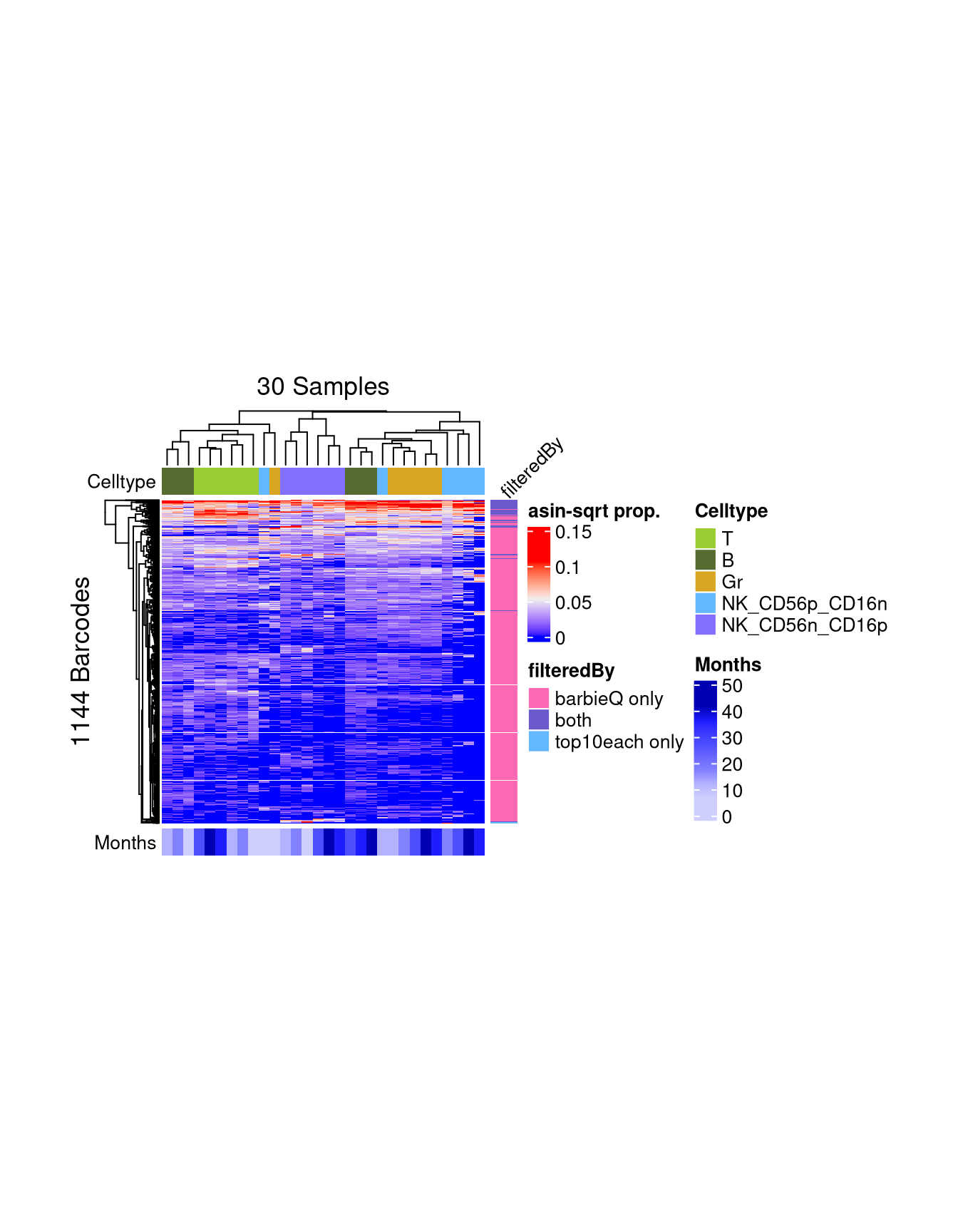

Version	Author	Date
dfa737a	FeiLiyang	2025-12-17

matrix color is mapped to `asin-sqrt proportion` but labeled by raw proportion.

## ht_filter@heatmap_param[["calling_env"]][["sampleAnnotation"]]@anno_list[["Months"]]@show_legend <- FALSE
## ht_filter@heatmap_param[["calling_env"]][["groupAnnotation"]]@anno_list[["Celltype"]]@show_legend <- FALSE

f4e <- draw(ht_filter, row_split = region_labels$region, width = unit(6, "cm"), height = unit(15, "cm")) %>%
  grid.grabExpr() %>% list() %>% wrap_plots()

'width' should not be set in draw() for horizontal heatmap list (Note a
single heatmap is a horizontal heatmap list). Please directly set it in
`Heatmap()`.

f4e <- Heatmap(
  monkeyHSPC_compare_filter@assays@data$proportion %>% sqrt() %>% asin(), name = "asin-sqrt prop.",
  cluster_rows = TRUE, cluster_columns = TRUE, show_row_names = FALSE, show_column_names = FALSE, 
  right_annotation = rowAnnotation(
    filteredBy = region_labels$region,
    col = list(filteredBy = c("barbieQ only" = "hotpink", "both" = "slateblue", "top10each only" = "steelblue1")),
    annotation_name_side = "top", annotation_name_rot = 45),
  row_split = region_labels$region, width = unit(6, "cm"), height = unit(15, "cm"), row_title = "Barcodes",
  top_annotation = HeatmapAnnotation(
    Celltype = monkeyHSPC_compare_filter$sampleMetadata$Celltype,
    Months = monkeyHSPC_compare_filter$sampleMetadata$Months,
    col = monkeyHSPC_compare_filter@metadata$factorColors,
    show_legend = FALSE, annotation_name_side = "left"
  ))

The automatically generated colors map from the 1^st and 99^th of the
values in the matrix. There are outliers in the matrix whose patterns
might be hidden by this color mapping. You can manually set the color
to `col` argument.

Use `suppressMessages()` to turn off this message.

f4e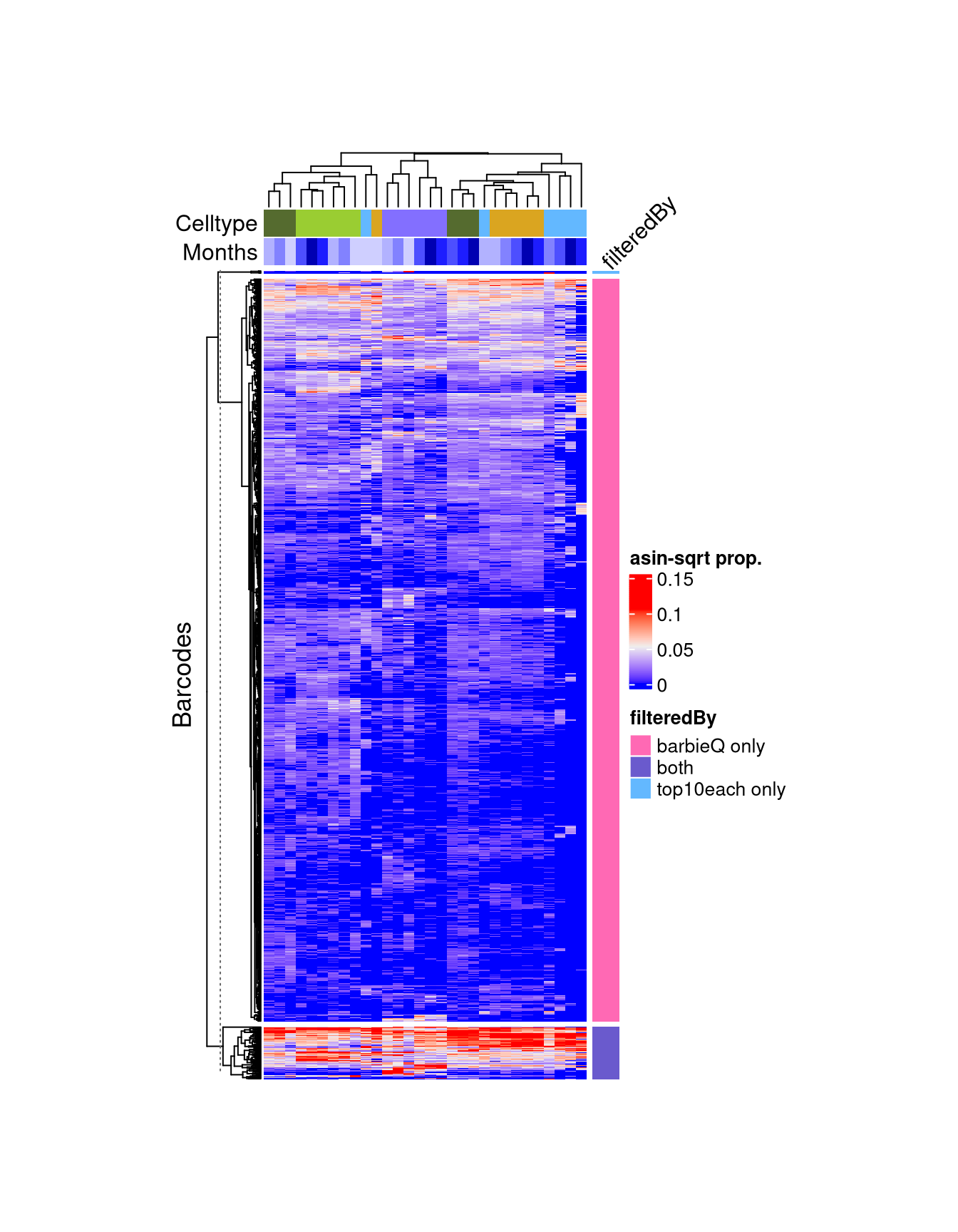

Version	Author	Date
dfa737a	FeiLiyang	2025-12-17

8 Compare difference identification on top10each filtering approach

8.1 barbieQ filter + barbieQ test

monkeyHSPC_top10each@elementMetadata$isTopBarcode$isTop %>% table()

.
FALSE  TRUE 
16519    79

## subset the 79 barcodes filtered by top10each
monkeyHSPC_top10each_79 <- monkeyHSPC_top10each[monkeyHSPC_top10each@elementMetadata$isTopBarcode$isTop,]
##need to take Time into account
designs <- monkeyHSPC_top10each_79$sampleMetadata %>% as.data.frame() %>%
  mutate(Months = as.factor(Months)) %>% 
  with(model.matrix(~0+ Celltype + Months))

monkeyHSPC_top10each_79 <- testBarcodeSignif(
  barbieQ = monkeyHSPC_top10each_79, designMatrix = designs,
  contrastFormula = "(CelltypeNK_CD56n_CD16p) - (CelltypeB+CelltypeGr+CelltypeT+CelltypeNK_CD56p_CD16n)/4",
  method = "diffProp", transformation = "asin-sqrt"
)

setting Celltype as the primary factor in `sampleMetadata`.

deleting 3 nested factor(s) because `designMatrix` must be full rank.

no block specified, so there are no duplicate measurements.

# check design
monkeyHSPC_top10each_79@elementMetadata$testingBarcode@metadata$contrasts

                        Contrasts
Levels                   (CelltypeNK_CD56n_CD16p) - (CelltypeB+CelltypeGr+CelltypeT+CelltypeNK_CD56p_CD16n)/4
  CelltypeT                                                                                             -0.25
  CelltypeB                                                                                             -0.25
  CelltypeGr                                                                                            -0.25
  CelltypeNK_CD56p_CD16n                                                                                -0.25
  CelltypeNK_CD56n_CD16p                                                                                 1.00
  Months12                                                                                               0.00
  Months17                                                                                               0.00
  Months27                                                                                               0.00
  Months36                                                                                               0.00
  Months42                                                                                               0.00

monkeyHSPC_top10each_79@elementMetadata$testingBarcode@metadata$design %>% data.table(keep.rownames = T)

8.2 barbieQ filter + LFC approach

1% contribution to CD56−CD16+ cells and
10-fold abundance in contribution to CD56−CD16+ cells compared with T, B, Gr, and CD56+CD16− cells.

calc_bias_LFC function sourced from “F4_validation.R”.

list_BC_top10each_LFC <- calc_bias_LFC(monkeyHSPC_top10each_79)
union_LFC_top10each <- unlist(list_BC_top10each_LFC) %>% unique()

## check overlaps between months
venn_top10each_LFC <- eulerr::euler(list_BC_top10each_LFC)
plot(venn_top10each_LFC, fills = c("white"), alpha = 0.5, labels = T, quantities = T)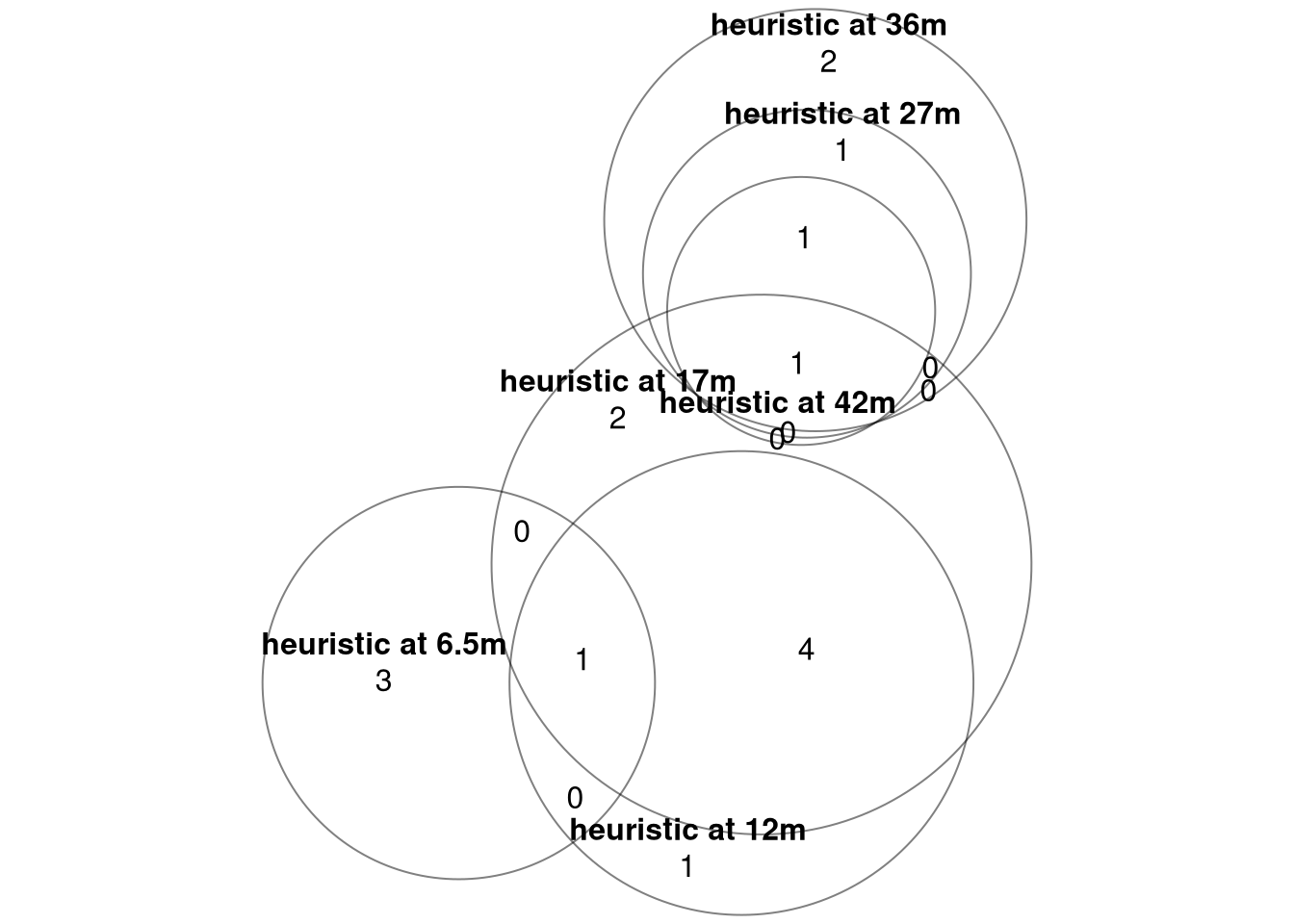

8.3 F4G: overlap

list_top10each_feature <- list(
    barbieQ = rownames(monkeyHSPC_top10each_79)[monkeyHSPC_top10each_79@elementMetadata$testingBarcode$tendencyTo == "CelltypeNK_CD56n_CD16p"],
    heuristics = union_LFC_top10each)

## plot Euler
# venn_top10each_feature <- eulerr::euler(list_top10each_feature) %>% 
#   plot(fills = c("pink","slateblue"),
#        alpha = 0.5, labels = list(font = 4, cex = 1), quantities = list(font = 1, cex = 1)) 
# 
# venn_top10each_feature %>% plot() %>% grid.grabExpr() %>% wrap_plots()

## plot UpSet plot
f4g <- list_top10each_feature %>% 
  Venn() %>% 
  plot_upset(top.bar.numbers.size = 4, relative_width = 0.0) ## limit left bar plot

## getting theme settings from an example ggplot using barbieQ theme
tester <- ggplot(data.frame(X = 1:3, Y = 4:6)) +
  geom_point(aes(x = X, y = Y)) +
  theme_barbieQ_size()

mytittle <- tester@theme$axis.title
mytext <- tester@theme$axis.text

## modifying components in UpSet plots: three gplot objects
f4g[["plotlist"]][[1]]@theme$axis.title <- mytittle
f4g[["plotlist"]][[1]]@theme$axis.text <- mytext

f4g[["plotlist"]][[2]]@theme$axis.title <- mytittle
f4g[["plotlist"]][[2]]@theme$axis.text <- mytext

f4g[["plotlist"]][[2]]@layers$geom_col$aes_params$width <- 0.4

f4g[["plotlist"]][[3]]@theme$axis.title <- mytittle
f4g[["plotlist"]][[3]]@theme$axis.text <- mytext

f4g[["plotlist"]][[3]]@theme$axis.text@size <- 11
f4g[["plotlist"]][[3]]@theme$axis.text@angle <- 15

## removing the left bar plot
f4g[["plotlist"]][[3]] <- f4g[["plotlist"]][[3]] + theme(
    panel.grid = element_blank(),
    axis.text = element_blank(),
    axis.title = element_blank(),
    axis.ticks = element_blank()
  )

## plot 4g
f4g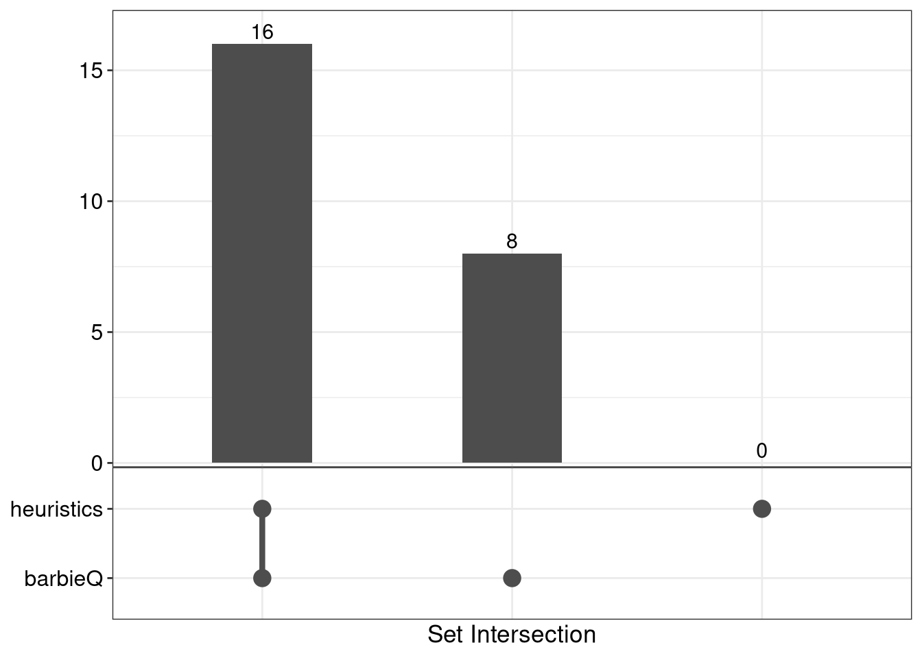

Version	Author	Date
dfa737a	FeiLiyang	2025-12-17

8.4 F4F: inspect two sets: boxplot

Box plot to visualize the LFC of sets of selected barcodes.

FC_top10each <- calc_bias_LFC(barbieQ = monkeyHSPC_top10each_79, get_FC = T) %>% as.data.frame()
rownames(FC_top10each) <- rownames(monkeyHSPC_top10each_79)
## annotating BC by barbieQ seletion
FC_top10each$bbq <- monkeyHSPC_top10each_79@elementMetadata$testingBarcode$direction
## annotating BC by heuristic selection
FC_top10each$heu = 0
FC_top10each[union_LFC_top10each, "heu"] = 1
  ## adding BC name
FC_top10each <- FC_top10each %>% 
  mutate(Barcode = rownames(monkeyHSPC_top10each_79)) %>% 
  ## summarizing two selecting methods overlaps
  mutate(identifiedBy = ifelse(bbq == 1, 
                             ifelse(heu == 1, "both", "barbieQ only"), 
                             ifelse(heu == 1, "heuristics only", "neither"))) %>% 
  dplyr::select(-c(heu, bbq))

## extract FC from testing
coff_FC <- monkeyHSPC_top10each_79@elementMetadata$testingBarcode$meanDiff
FC_top10each$testing_coeff <- coff_FC

long_FC_top10each <- FC_top10each %>% 
  mutate(Barcode = rownames(monkeyHSPC_top10each_79)) %>% 
  pivot_longer(
      cols = -c(Barcode, identifiedBy, testing_coeff),     # keep Celltype and Months fixed
      names_to = "Month",
      values_to = "FC"
    )

Draw box plot, barcodes ordered by mean LFC

## order BC in x axis by contrast coefficient
barcode_order <- long_FC_top10each %>%
  group_by(Barcode) %>%
  summarise(mean_LFC = mean((testing_coeff), na.rm = TRUE)) %>%
  arrange(mean_LFC) %>%
  pull(Barcode)

long_FC_top10each$identifiedBy <- factor(
  long_FC_top10each$identifiedBy,
  levels = c("barbieQ only", "heuristics only", "both", "neither")
)

## remove level "heuristics only"
long_FC_top10each$identifiedBy <- factor(
  long_FC_top10each$identifiedBy,
  levels = c("barbieQ only",  "both", "neither")
)

p_box_coef <- ggplot(long_FC_top10each, aes(x = factor(Barcode, levels = barcode_order), y = log2(FC), group = (Barcode), color = identifiedBy)) +
  geom_boxplot(varwidth = T) +
  # geom_jitter()+
  theme_classic() +
  theme(axis.text.x = element_blank(), legend.position = "right", axis.title = element_text(size = 14)) +
  geom_abline(slope = 0, intercept = 0, linetype = 2, colour = "snow4") +
  labs(x = "",
       y = "LFC",
       title = "Barocdes selected by top10each filtering") +
  scale_color_manual(
    values = c("both" = "slateblue", "barbieQ only" = "hotpink", "heuristics only" = "steelblue1", "neither" = "slategray"),
    drop = FALSE)

p_box_coef_2 <- ggplot(long_FC_top10each, aes(x = factor(Barcode, levels = barcode_order), y = testing_coeff, group = (Barcode), color = identifiedBy)) +
  geom_boxplot(varwidth = T) +
  theme_classic() +
  theme(axis.text.x = element_blank(), legend.position = "none", axis.title = element_text(size = 14)) +
  geom_abline(slope = 0, intercept = 0, linetype = 2, colour = "snow4") +
  labs(x = "Barocdes ordered by barbieQ-estimated size effect",
       y = "Size effect") +
  scale_color_manual(values = c("both" = "slateblue", "barbieQ only" = "hotpink", "heuristics only" = "steelblue1", "neither" = "slategray"))

f4f <- p_box_coef / p_box_coef_2 + plot_layout(heights = c(3, 1))
f4f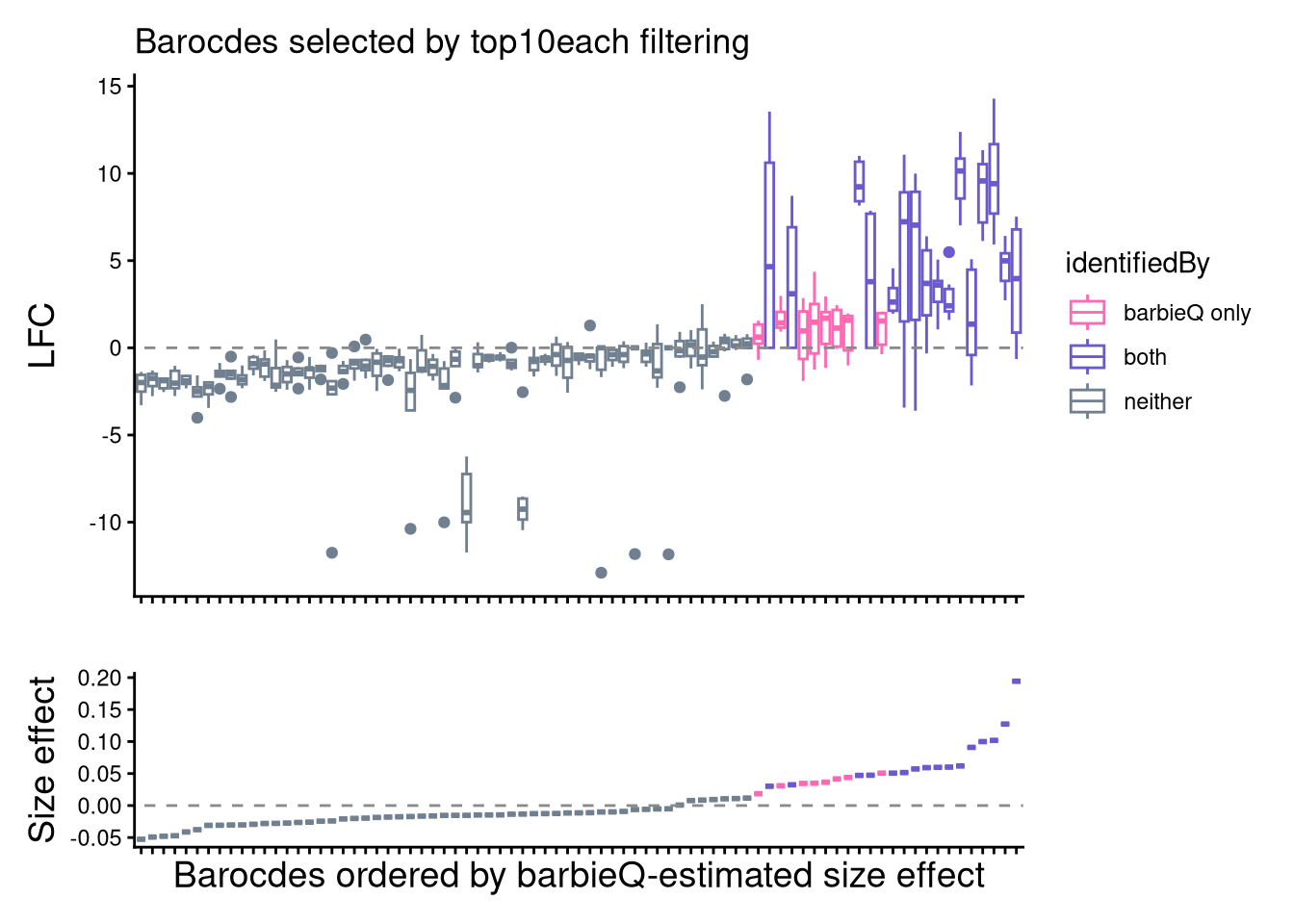

9 Compare fitering with barbieQ testing

9.1 top10each + barbieQ test

##need to take Time into account
designs <- monkeyHSPC_merged_top$sampleMetadata %>% as.data.frame() %>%
  mutate(Months = as.factor(Months)) %>% 
  with(model.matrix(~0+ Celltype + Months))

monkeyHSPC_merged_top <- testBarcodeSignif(
  barbieQ = monkeyHSPC_merged_top, designMatrix = designs,
  contrastFormula = "(CelltypeNK_CD56n_CD16p) - (CelltypeB+CelltypeGr+CelltypeT+CelltypeNK_CD56p_CD16n)/4",
  method = "diffProp", transformation = "asin-sqrt"
)

setting Celltype as the primary factor in `sampleMetadata`.

deleting 3 nested factor(s) because `designMatrix` must be full rank.

no block specified, so there are no duplicate measurements.

# check design
monkeyHSPC_merged_top@elementMetadata$testingBarcode@metadata$contrasts

                        Contrasts
Levels                   (CelltypeNK_CD56n_CD16p) - (CelltypeB+CelltypeGr+CelltypeT+CelltypeNK_CD56p_CD16n)/4
  CelltypeT                                                                                             -0.25
  CelltypeB                                                                                             -0.25
  CelltypeGr                                                                                            -0.25
  CelltypeNK_CD56p_CD16n                                                                                -0.25
  CelltypeNK_CD56n_CD16p                                                                                 1.00
  Months12                                                                                               0.00
  Months17                                                                                               0.00
  Months27                                                                                               0.00
  Months36                                                                                               0.00
  Months42                                                                                               0.00

monkeyHSPC_merged_top@elementMetadata$testingBarcode@metadata$design %>% data.table(keep.rownames = T)

9.2 F4H: stacked proportion

plot_validation sourced from “F4_validation.R”

 f4h <- (plot_validation(monkeyHSPC_top10each_79) + 
    theme( plot.title = element_text(hjust = 0.5, vjust = 1)) + labs(title = "Based on top10each")) +
  (plot_validation(monkeyHSPC_merged_top) + 
     theme( plot.title = element_text(hjust = 0.5, vjust = 1)) + labs(title = "Based on barbieQ"))

f4h

Warning: Removed 5 rows containing missing values or values outside the scale range
(`geom_bar()`).

Warning: Removed 5 rows containing missing values or values outside the scale range
(`geom_tile()`).

Warning: Removed 5 rows containing missing values or values outside the scale range
(`geom_bar()`).

Warning: Removed 5 rows containing missing values or values outside the scale range
(`geom_tile()`).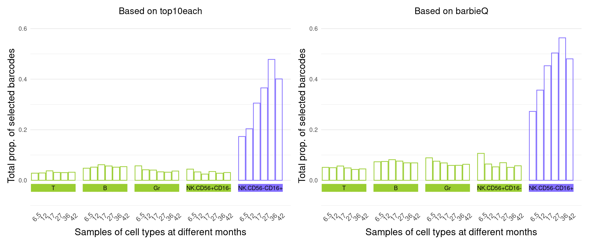

9.3 overlap

compare sets of significant barcodes

## signif. BC
filter_venn_signif_list <- list(
  ## signif. BC
  top10each = rownames(monkeyHSPC_top10each_79)[monkeyHSPC_top10each_79@elementMetadata$testingBarcode$tendencyTo == "CelltypeNK_CD56n_CD16p"],
  barbieQ = rownames(monkeyHSPC_merged_top)[monkeyHSPC_merged_top@elementMetadata$testingBarcode$tendencyTo == "CelltypeNK_CD56n_CD16p"],
  ## all BC in test
  top10each_all = rownames(monkeyHSPC_top10each_79),
  barbieQ_filter_all = rownames(monkeyHSPC_merged_top))

venn_filter_signif <- eulerr::euler(filter_venn_signif_list[1:2]) %>% 
  plot(fills = c("skyblue", "pink"), 
       alpha = 0.5, labels = list(font = 4, cex = 1), quantities = list(font = 1, cex = 1))

venn_filter_signif  %>% plot() %>% grid.grabExpr() %>% wrap_plots()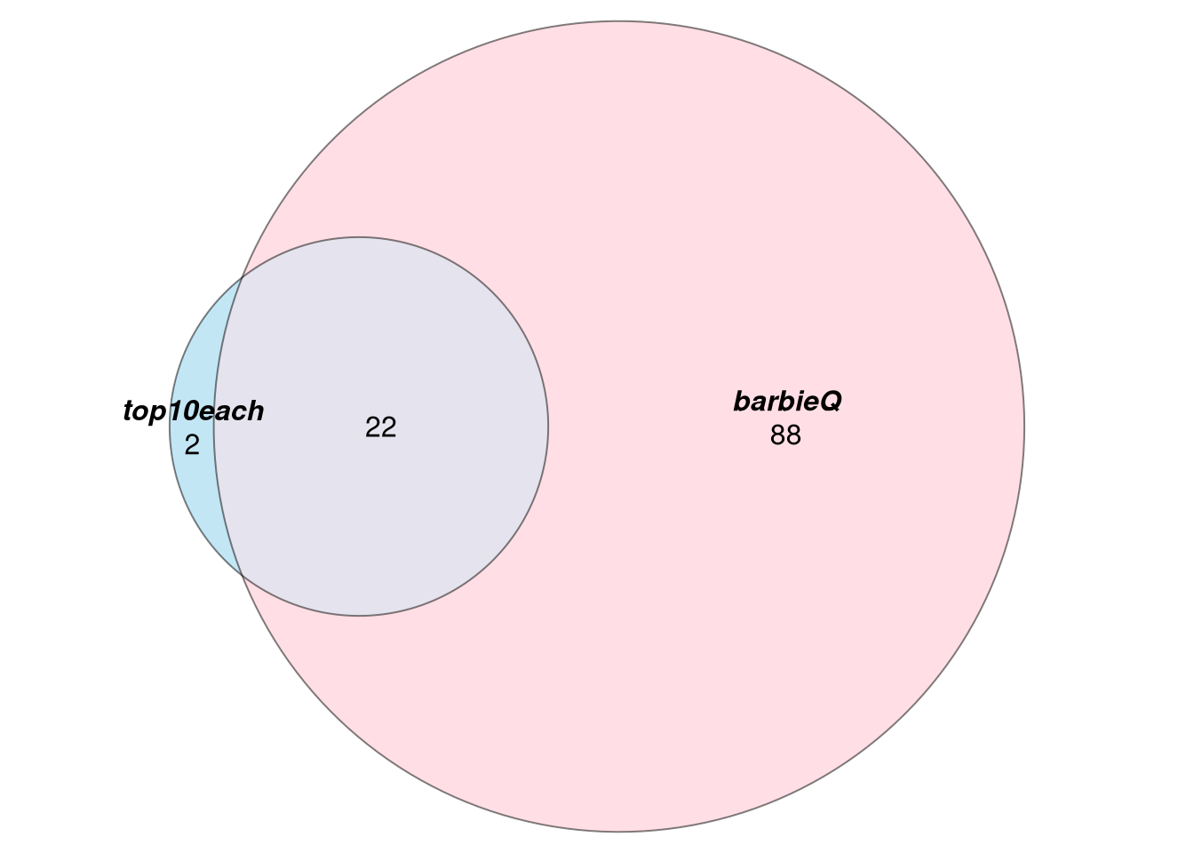

Version	Author	Date
dfa737a	FeiLiyang	2025-12-17

9.4 F4I: inspect two sets: boxplot

box plot on two sets of significant barcodes based on two filtering appraoches

BC_filter_sig <- filter_venn_signif_list[1:2] %>% unlist %>% unique()

FC_filter_sig <- calc_bias_LFC(barbieQ = monkeyHSPC_merged[BC_filter_sig,], get_FC = T) %>% 
  as.data.frame()
Mean_filter_sig <- calc_bias_LFC(barbieQ = monkeyHSPC_merged[BC_filter_sig,], get_AMean = T) %>%
  as.data.frame()
rownames(FC_filter_sig) <- BC_filter_sig
## annotating BC by barbieQ seletion
FC_filter_sig$top10each = 0
FC_filter_sig$bbq = 0
## annotating BC by heuristic selection, `filter_venn_signif_list` obtained from last chunk
FC_filter_sig[filter_venn_signif_list[[1]], "top10each"] = 1
FC_filter_sig[filter_venn_signif_list[[2]], "bbq"] = 1
  ## adding BC name
FC_filter_sig <- FC_filter_sig %>% 
  mutate(Barcode = BC_filter_sig) %>% 
  ## summarizing two selecting methods overlaps
  mutate(FilteringMethod = ifelse(top10each == 1, 
                                  ifelse(bbq == 1, "both", "top10each"),
                                  ifelse(bbq == 1, "barbieQ", "neither"))) %>% 
  dplyr::select(-c(top10each, bbq))

## extract FC from testing

long_FC_filter_sig <- FC_filter_sig %>% 
  mutate(Barcode = BC_filter_sig) %>% 
  pivot_longer(
      cols = -c(Barcode, FilteringMethod),     # keep Celltype and Months fixed
      names_to = "Month",
      values_to = "FC"
    )
# Add barcode column to Mean_filter_sig
Mean_filter_sig <- Mean_filter_sig %>%
  mutate(Barcode = BC_filter_sig)

long_Mean <- Mean_filter_sig %>%
  pivot_longer(
    cols = -Barcode,
    names_to = "Month",
    values_to = "Mean"
  )

long_FC_filter_sig <- long_FC_filter_sig %>%
  left_join(long_Mean, by = c("Barcode", "Month"))

barcode_order_filter_sig <- long_FC_filter_sig %>%
  group_by(Barcode) %>%
  summarise(AMean = mean(Mean, na.rm = TRUE)) %>%
  arrange(AMean) %>%
  pull(Barcode)

barcode_order_df_filter_sig <- long_FC_filter_sig %>%
  group_by(Barcode, FilteringMethod) %>%
  summarise(AMean = mean(Mean, na.rm = TRUE)) %>%
  arrange(AMean)

`summarise()` has grouped output by 'Barcode'. You can override using the
`.groups` argument.

p_AMean_0 <- ggplot()+
  geom_point(data = barcode_order_df_filter_sig,
             aes(x = factor(Barcode, levels = barcode_order_filter_sig),
                 y = log10(AMean),
                 color = FilteringMethod),
             size = 1.5, shape = 15,
             inherit.aes = FALSE) +
  theme_classic() +
  theme(axis.text.x = element_blank(), legend.position = "none", axis.title = element_text(size = 14)) +
  labs(x = "Barocdes ordered by mean proportion across cell types across time",
       y = "Log10 prop.") +
  scale_color_manual(values = c("both" = "slateblue", "barbieQ" = "hotpink", "top10each" = "steelblue1"))


p_box_0 <- ggplot(long_FC_filter_sig, aes(x = factor(Barcode, levels = barcode_order_filter_sig), y = log2(FC), group = (Barcode), color = FilteringMethod)) +
  geom_boxplot(varwidth = T) +
  theme_classic() +
  theme(axis.text.x = element_blank(), legend.position = "right", axis.title = element_text(size = 14)) +
  geom_abline(slope = 0, intercept = 0, linetype = 2, colour = "grey") +
  labs(x = "",
       y = "LFC",
       title = "Barcodes significant in barbieQ test, selected by either barbieQ or top10each filtering") +
  scale_color_manual(values = c("both" = "slateblue", "barbieQ" = "hotpink", "top10each" = "steelblue1"))

f4i <- p_box_0 / p_AMean_0 + plot_layout(heights = c(3, 1))
f4i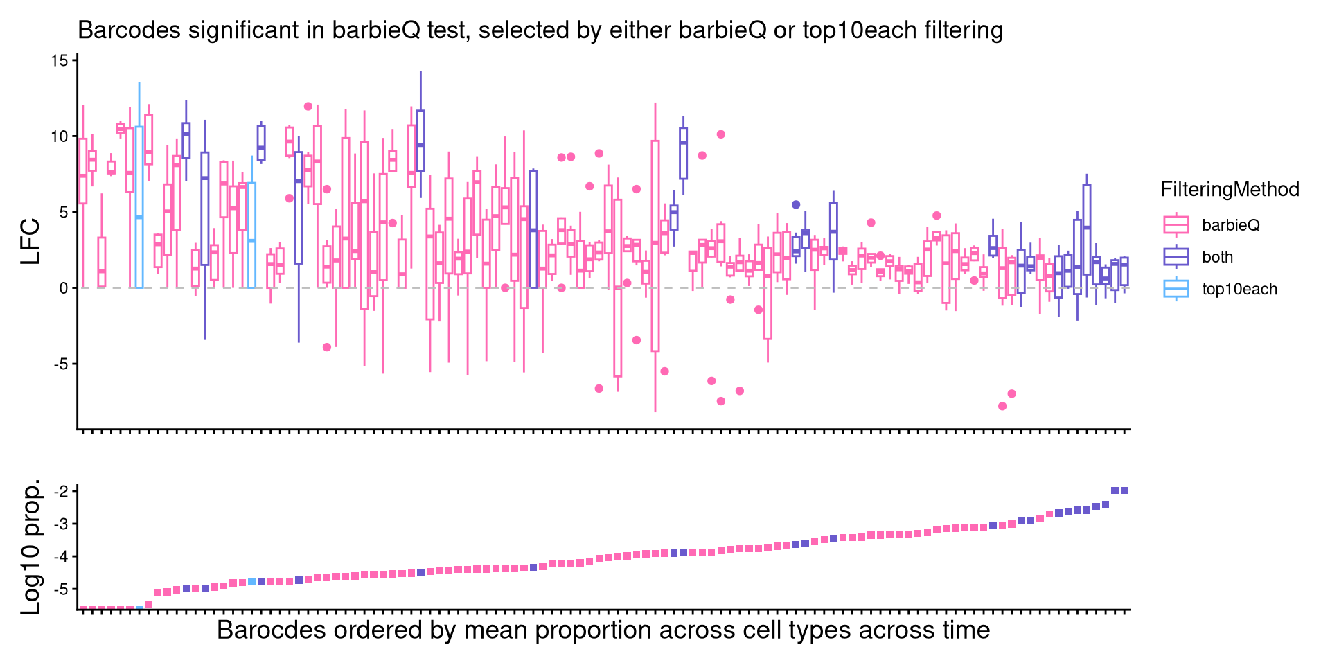

10 F4J: Example difference over time

designs <- monkeyHSPC_top10each_79$sampleMetadata %>% as.data.frame() %>%
  with(model.matrix(~0+ Celltype+ Celltype:Months))
designs <- designs[,c(1:5, 9:13)]
colnames(designs) <- gsub(":", ".", colnames(designs))

monkeyHSPC_top10each_79_NK <- testBarcodeSignif(
  barbieQ = monkeyHSPC_top10each_79, 
  sampleMetadata = designs, designMatrix = designs, sampleGroup = "CelltypeNK_CD56n_CD16p.Months",
  method = "diffProp", transformation = "asin-sqrt"
)

setting CelltypeNK_CD56n_CD16p.Months as the primary factor in `sampleMetadata`.

setting up contrastFormula: CelltypeNK_CD56n_CD16p.Months

no block specified, so there are no duplicate measurements.

monkeyHSPC_top10each_79_NK@elementMetadata$testingBarcode$tendencyTo %>% table()

.
CelltypeNK_CD56n_CD16p.Monthsdowntrend   CelltypeNK_CD56n_CD16p.Monthsuptrend 
                                    16                                     16 
                                  n.s. 
                                    47

monkeyHSPC_top10each_79_NK@elementMetadata$testingBarcode@metadata$design %>% data.table()

monkeyHSPC_top10each_79_NK@elementMetadata$testingBarcode@metadata$contrasts

                               Contrasts
Levels                          CelltypeNK_CD56n_CD16p.Months
  CelltypeT                                                 0
  CelltypeB                                                 0
  CelltypeGr                                                0
  CelltypeNK_CD56p_CD16n                                    0
  CelltypeNK_CD56n_CD16p                                    0
  CelltypeT.Months                                          0
  CelltypeB.Months                                          0
  CelltypeGr.Months                                         0
  CelltypeNK_CD56p_CD16n.Months                             0
  CelltypeNK_CD56n_CD16p.Months                             1

monkeyHSPC_top10each_79_NK@elementMetadata$testingBarcode@metadata$contrastGroups

                                levelLow 
"CelltypeNK_CD56n_CD16p.Monthsdowntrend" 
                               levelHigh 
  "CelltypeNK_CD56n_CD16p.Monthsuptrend"

NKnp_fig <- monkeyHSPC_top10each_79_NK[,monkeyHSPC_top10each_79_NK$sampleMetadata$Celltype == "NK_CD56n_CD16p"]

BC_kinetic <- NKnp_fig@elementMetadata$testingBarcode$tendencyTo

pch_fun <- ifelse(NKnp_fig@elementMetadata$testingBarcode$direction != 0, "*", NA)

kinetic_ha <- rowAnnotation(
  Kinetic = anno_simple(
    BC_kinetic,
    col = NKnp_fig@metadata$factorColors$testingBarcode,
    pch = pch_fun
    ),
  show_annotation_name = TRUE,
  annotation_name_side = "top",
  annotation_name_rot = 45
)

HP_anno_kinetic <- Heatmap(
  asin(sqrt(NKnp_fig@assays@data$proportion)), name = "asin-sqrt prop.",
  show_row_names = FALSE, column_labels = NKnp_fig$sampleMetadata$Months,
  column_title = "Months", column_names_side = "top", column_names_rot = 45,
  row_title = "Barcodes", row_km = 4,
  width = unit(4, "cm"), height = unit(12, "cm"),
  column_order = order(NKnp_fig$sampleMetadata$Months),
  # col = colorRamp2(c(0, -2, -4.602), c("red", "white", "blue")),
  # left_annotation = row_ha,
  right_annotation = kinetic_ha
)

The automatically generated colors map from the 1^st and 99^th of the
values in the matrix. There are outliers in the matrix whose patterns
might be hidden by this color mapping. You can manually set the color
to `col` argument.

Use `suppressMessages()` to turn off this message.

lgd_sig = Legend(pch = "*", type = "points", labels = "signif.")

lgd_kinetic = Legend(labels = c("up", "down", "n.s."), title = "Kinetic", 
             legend_gp = gpar(fill = c("#FF5959", "#33AAFF", "#FFC000"))
             )
## heatmap_legend_side = "top", annotation_legend_side = "top"

f4j <- draw(HP_anno_kinetic, annotation_legend_list = list(lgd_kinetic, lgd_sig),
            annotation_legend_side = "bottom", heatmap_legend_side = "bottom") %>%
  grid.grabExpr() %>% list() %>% wrap_plots()

f4j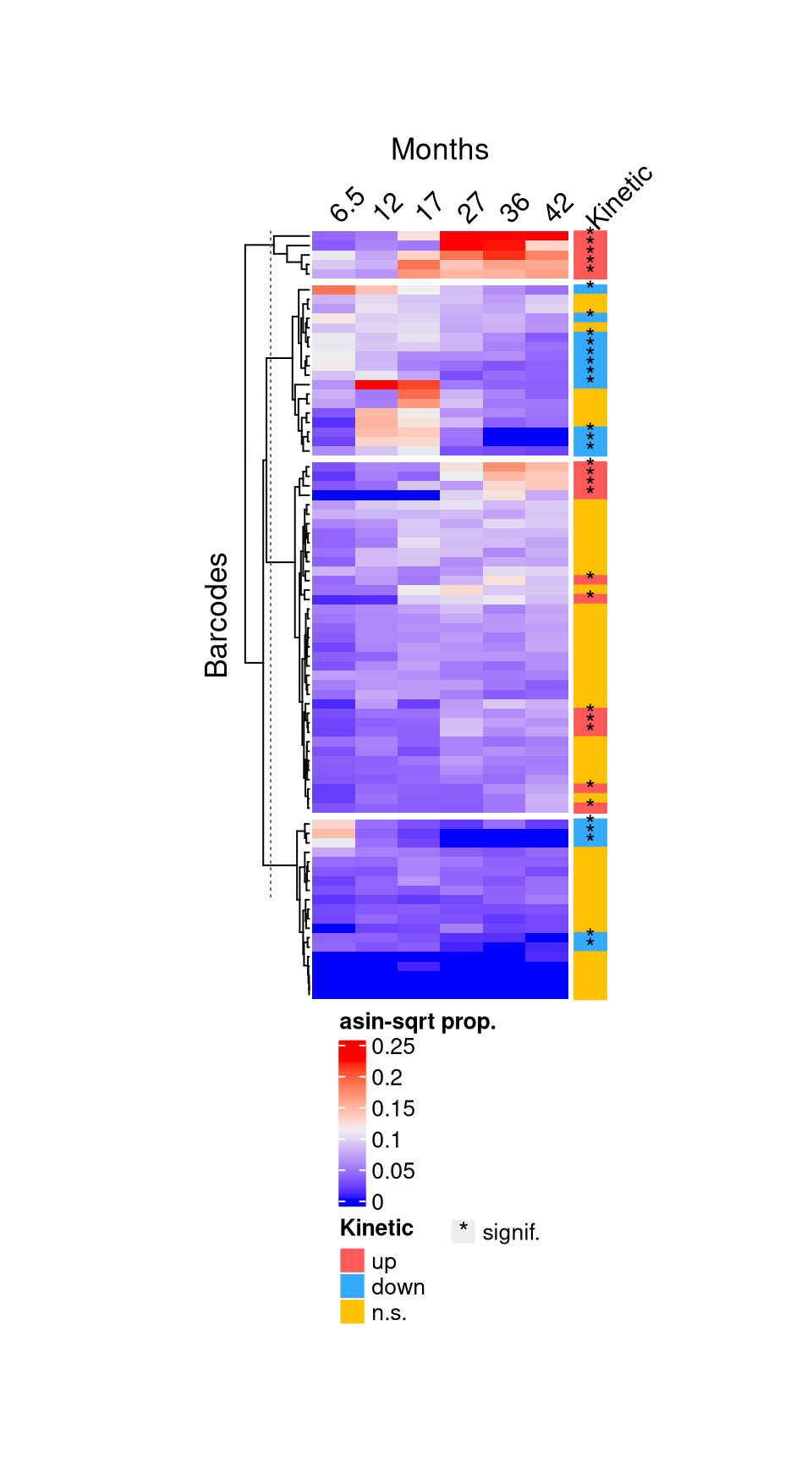

Version	Author	Date
dfa737a	FeiLiyang	2025-12-17

11 Figure 4

layout = "
AAAAAAAAAAAAA##
AAAAAAAAAAAAA##
BBBBBBCCCCEEEEE
BBBBBBCCCCEEEEE
BBBBBBCCCCEEEEE
DDDDDDDDDDEEEEE
DDDDDDDDDDEEEEE
DDDDDDDDDDEEEEE
FFFFFFFFFFGGGG#
FFFFFFFFFFGGGG#
FFFFFFFFFFGGGG#
HHHHHHHHHHJJJJ#
HHHHHHHHHHJJJJ#
HHHHHHHHHHJJJJ#
HHHHHHHHHHJJJJ#
IIIIIIIIIIJJJJ#
IIIIIIIIIIJJJJ#
IIIIIIIIIIJJJJ#
"
f4 <- (wrap_elements(full = f4a) + 
    wrap_elements(f4b + theme(plot.margin = unit(rep(0,4), "cm"))) + 
    wrap_elements(grid.grabExpr(print(f4c))) +
    wrap_elements(f4d + theme(plot.margin = unit(rep(0,4), "cm"))) +
    wrap_plots(list(f4e %>% draw() %>% grid.grabExpr())) +
    wrap_elements(f4f + theme(plot.margin = unit(rep(0,4), "cm"))) + 
    wrap_elements(grid.grabExpr(print(f4g))) + 
    wrap_elements(f4h + theme(plot.margin = unit(c(0,0,0,0), "cm"))) +
    wrap_elements(f4i + theme(plot.margin = unit(rep(0,4), "cm"))) +
    # wrap_elements(f4j + theme(plot.margin = unit(rep(0,4), "cm")))
  wrap_plots(list(HP_anno_kinetic %>% 
          draw(annotation_legend_list = list(lgd_kinetic, lgd_sig), 
               annotation_legend_side = "top",heatmap_legend_side = "top") %>% 
            grid.grabExpr()))
    )+ 
  plot_layout(design = layout) +
  plot_annotation(tag_levels = list(c("A","B","C", "D", "E","F","G","H", "I", "J"))) &
  theme(
    plot.tag = element_text(size = 24, face = "bold", family = "arial"),
    axis.title = element_text(size = 20),
    axis.text = element_text(size = 14),
    legend.title = element_text(size = 13),
    legend.text = element_text(size = 11))

f4

Warning: Removed 5 rows containing missing values or values outside the scale range
(`geom_bar()`).

Warning: Removed 5 rows containing missing values or values outside the scale range
(`geom_tile()`).

Warning: Removed 5 rows containing missing values or values outside the scale range
(`geom_bar()`).

Warning: Removed 5 rows containing missing values or values outside the scale range
(`geom_tile()`).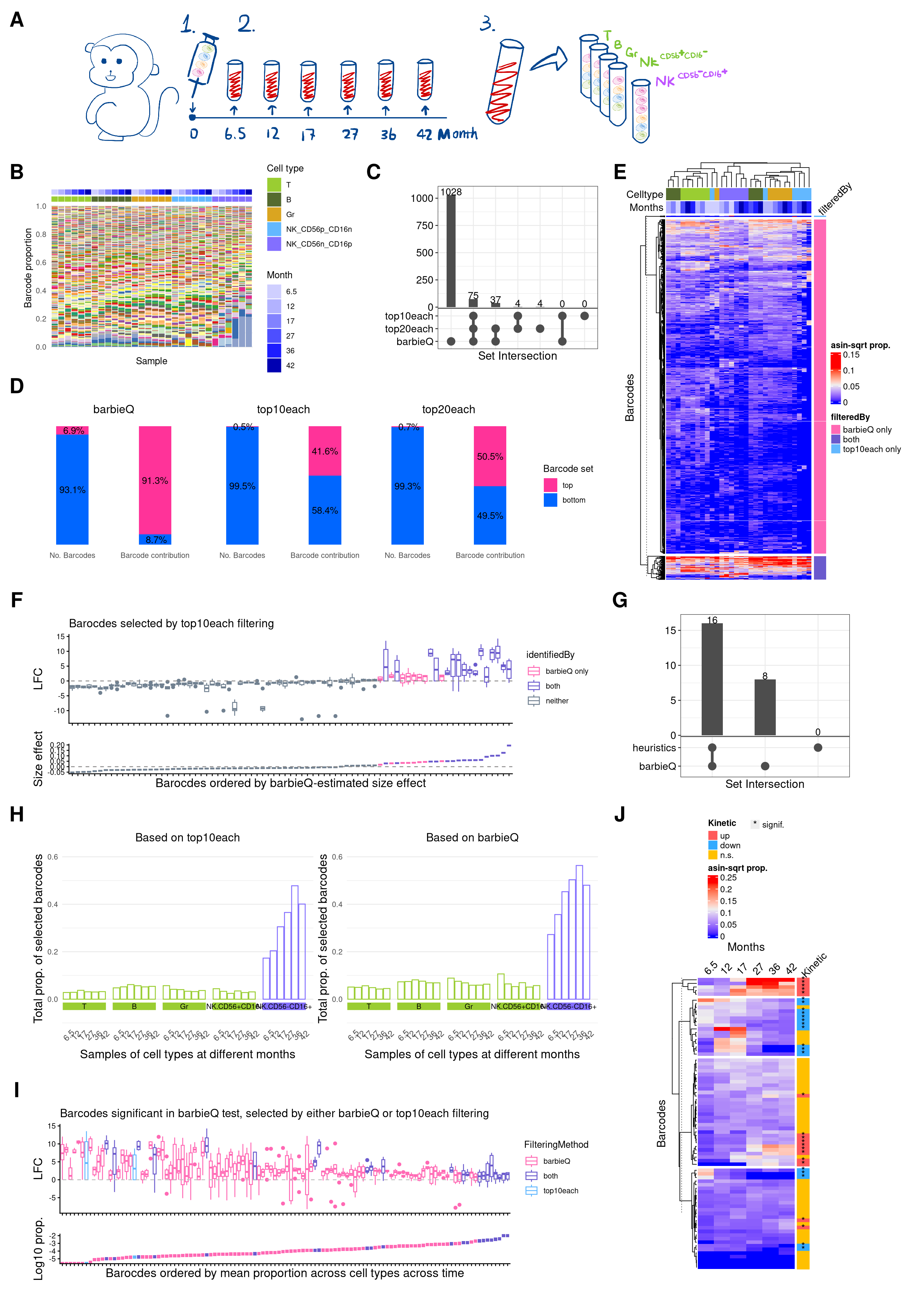

Version	Author	Date
dfa737a	FeiLiyang	2025-12-17

ggsave(
  filename = "output/f4.png",
  plot = f4,
  width = 15,
  height = 21,
  units = "in", # for Rmd r chunk fig size, unit default to inch
  dpi = 350
  )

Warning: Removed 5 rows containing missing values or values outside the scale range
(`geom_bar()`).

Warning: Removed 5 rows containing missing values or values outside the scale range
(`geom_tile()`).

Warning: Removed 5 rows containing missing values or values outside the scale range
(`geom_bar()`).

Warning: Removed 5 rows containing missing values or values outside the scale range
(`geom_tile()`).

Saving this figure in f4

sessionInfo()

R version 4.5.0 (2025-04-11)
Platform: x86_64-pc-linux-gnu
Running under: Red Hat Enterprise Linux 9.6 (Plow)

Matrix products: default
BLAS/LAPACK: FlexiBLAS OPENBLAS-OPENMP;  LAPACK version 3.9.0

locale:
 [1] LC_CTYPE=en_AU.UTF-8       LC_NUMERIC=C              
 [3] LC_TIME=en_AU.UTF-8        LC_COLLATE=en_AU.UTF-8    
 [5] LC_MONETARY=en_AU.UTF-8    LC_MESSAGES=en_AU.UTF-8   
 [7] LC_PAPER=en_AU.UTF-8       LC_NAME=C                 
 [9] LC_ADDRESS=C               LC_TELEPHONE=C            
[11] LC_MEASUREMENT=en_AU.UTF-8 LC_IDENTIFICATION=C       

time zone: Australia/Melbourne
tzcode source: system (glibc)

attached base packages:
[1] grid      stats4    stats     graphics  grDevices utils     datasets 
[8] methods   base     

other attached packages:
 [1] barbieQ_1.1.3               edgeR_4.6.3                
 [3] limma_3.64.3                eulerr_7.0.4               
 [5] magick_2.9.0                ComplexHeatmap_2.24.1      
 [7] ggVennDiagram_1.5.4         scales_1.4.0               
 [9] patchwork_1.3.2             ggnewscale_0.5.2           
[11] ggbreak_0.1.6               ggplot2_4.0.0              
[13] SummarizedExperiment_1.38.1 Biobase_2.68.0             
[15] GenomicRanges_1.60.0        GenomeInfoDb_1.44.3        
[17] IRanges_2.42.0              S4Vectors_0.48.0           
[19] BiocGenerics_0.54.0         generics_0.1.4             
[21] MatrixGenerics_1.20.0       matrixStats_1.5.0          
[23] data.table_1.17.8           knitr_1.50                 
[25] tibble_3.3.0                tidyr_1.3.1                
[27] dplyr_1.1.4                 magrittr_2.0.4             
[29] readxl_1.4.5                workflowr_1.7.2            

loaded via a namespace (and not attached):
  [1] RColorBrewer_1.1-3      rstudioapi_0.17.1       jsonlite_2.0.0         
  [4] shape_1.4.6.1           jomo_2.7-6              nloptr_2.2.1           
  [7] farver_2.1.2            logistf_1.26.1          rmarkdown_2.30         
 [10] ragg_1.5.0              GlobalOptions_0.1.2     fs_1.6.6               
 [13] vctrs_0.6.5             minqa_1.2.8             memoise_2.0.1          
 [16] forcats_1.0.1           htmltools_0.5.8.1       S4Arrays_1.8.1         
 [19] broom_1.0.10            cellranger_1.1.0        SparseArray_1.8.1      
 [22] gridGraphics_0.5-1      mitml_0.4-5             sass_0.4.10            
 [25] bslib_0.9.0             cachem_1.1.0            whisker_0.4.1          
 [28] igraph_2.1.4            lifecycle_1.0.4         iterators_1.0.14       
 [31] pkgconfig_2.0.3         Matrix_1.7-3            R6_2.6.1               
 [34] fastmap_1.2.0           rbibutils_2.3           GenomeInfoDbData_1.2.14
 [37] clue_0.3-66             digest_0.6.37           aplot_0.2.9            
 [40] colorspace_2.1-2        ps_1.9.1                rprojroot_2.1.1        
 [43] textshaping_1.0.3       labeling_0.4.3          httr_1.4.7             
 [46] polyclip_1.10-7         abind_1.4-8             mgcv_1.9-1             
 [49] compiler_4.5.0          withr_3.0.2             doParallel_1.0.17      
 [52] backports_1.5.0         S7_0.2.0                viridis_0.6.5          
 [55] ggforce_0.5.0           pan_1.9                 MASS_7.3-65            
 [58] rappdirs_0.3.3          DelayedArray_0.34.1     rjson_0.2.23           
 [61] tools_4.5.0             httpuv_1.6.16           nnet_7.3-20            
 [64] glue_1.8.0              callr_3.7.6             nlme_3.1-168           
 [67] promises_1.3.3          polylabelr_0.3.0        getPass_0.2-4          
 [70] cluster_2.1.8.1         operator.tools_1.6.3    gtable_0.3.6           
 [73] formula.tools_1.7.1     tidygraph_1.3.1         XVector_0.48.0         
 [76] ggrepel_0.9.6           foreach_1.5.2           pillar_1.11.1          
 [79] stringr_1.5.2           yulab.utils_0.2.1       later_1.4.4            
 [82] circlize_0.4.16         splines_4.5.0           tweenr_2.0.3           
 [85] lattice_0.22-6          survival_3.8-3          tidyselect_1.2.1       
 [88] locfit_1.5-9.12         git2r_0.36.2            reformulas_0.4.1       
 [91] gridExtra_2.3           xfun_0.53               graphlayouts_1.2.2     
 [94] statmod_1.5.0           stringi_1.8.7           UCSC.utils_1.4.0       
 [97] boot_1.3-31             ggfun_0.2.0             yaml_2.3.10            
[100] evaluate_1.0.5          codetools_0.2-20        ggraph_2.2.2           
[103] ggplotify_0.1.3         cli_3.6.5               rpart_4.1.24           
[106] systemfonts_1.3.1       Rdpack_2.6.4            processx_3.8.6         
[109] jquerylib_0.1.4         Rcpp_1.1.0              png_0.1-8              
[112] parallel_4.5.0          lme4_1.1-37             glmnet_4.1-10          
[115] viridisLite_0.4.2       purrr_1.1.0             crayon_1.5.3           
[118] GetoptLong_1.0.5        rlang_1.1.6             mice_3.18.0

barbieQ_paper_Figure4: Case study of `monkey HSPC`

Liyang Fei

Initiate: 2025-09-07

Last update: 2026-01-11

1 Load Dependencies

2 Install `barbieQ`

3 Set seeds

4 Load preprocessed data

5 F4A: Experimental schematic

6 F4B: Plot barcode proportion and sample annotation

7 Compare filtering

7.1 F4D: top10each vs. barbieQ filter

7.2 F4C: overlap

7.3 F4E: inspect two sets: heatmap

8 Compare difference identification on top10each filtering approach

8.1 barbieQ filter + barbieQ test

8.2 barbieQ filter + LFC approach

8.3 F4G: overlap

8.4 F4F: inspect two sets: boxplot

9 Compare fitering with barbieQ testing

9.1 top10each + barbieQ test

9.2 F4H: stacked proportion

9.3 overlap

9.4 F4I: inspect two sets: boxplot

10 F4J: Example difference over time

11 Figure 4

barbieQ_paper_Figure4: Case study of monkey HSPC

Liyang Fei

Initiate: 2025-09-07 Last update: 2026-01-11

1 Load Dependencies

2 Install barbieQ

3 Set seeds

4 Load preprocessed data

5 F4A: Experimental schematic

6 F4B: Plot barcode proportion and sample annotation

7 Compare filtering

7.1 F4D: top10each vs. barbieQ filter

7.2 F4C: overlap

7.3 F4E: inspect two sets: heatmap

8 Compare difference identification on top10each filtering approach

8.1 barbieQ filter + barbieQ test

8.2 barbieQ filter + LFC approach

8.3 F4G: overlap

8.4 F4F: inspect two sets: boxplot

9 Compare fitering with barbieQ testing

9.1 top10each + barbieQ test

9.2 F4H: stacked proportion

9.3 overlap

9.4 F4I: inspect two sets: boxplot

10 F4J: Example difference over time

11 Figure 4

barbieQ_paper_Figure4: Case study of `monkey HSPC`

Initiate: 2025-09-07

Last update: 2026-01-11

2 Install `barbieQ`