barbieQ_paper Supplementary 1:
Preprocessing Mixture data
Liyang Fei
Initiate: 2025-09-07
Last update: 2026-01-11
Last updated: 2026-01-11
Checks: 6 1
Knit directory: public_barcode_count/
This reproducible R Markdown analysis was created with workflowr (version 1.7.2). The Checks tab describes the reproducibility checks that were applied when the results were created. The Past versions tab lists the development history.
Great! Since the R Markdown file has been committed to the Git repository, you know the exact version of the code that produced these results.
The global environment had objects present when the code in the R
Markdown file was run. These objects can affect the analysis in your R
Markdown file in unknown ways. For reproduciblity it’s best to always
run the code in an empty environment. Use wflow_publish or
wflow_build to ensure that the code is always run in an
empty environment.
The following objects were defined in the global environment when these results were created:
| Name | Class | Size |
|---|---|---|
| module | function | 5.6 Kb |
The command set.seed(20250112) was run prior to running
the code in the R Markdown file. Setting a seed ensures that any results
that rely on randomness, e.g. subsampling or permutations, are
reproducible.
Great job! Recording the operating system, R version, and package versions is critical for reproducibility.
Nice! There were no cached chunks for this analysis, so you can be confident that you successfully produced the results during this run.
Great job! Using relative paths to the files within your workflowr project makes it easier to run your code on other machines.
Great! You are using Git for version control. Tracking code development and connecting the code version to the results is critical for reproducibility.
The results in this page were generated with repository version 670258c. See the Past versions tab to see a history of the changes made to the R Markdown and HTML files.
Note that you need to be careful to ensure that all relevant files for
the analysis have been committed to Git prior to generating the results
(you can use wflow_publish or
wflow_git_commit). workflowr only checks the R Markdown
file, but you know if there are other scripts or data files that it
depends on. Below is the status of the Git repository when the results
were generated:
Ignored files:
    Ignored:    .RData
    Ignored:    .Rhistory
    Ignored:    .Rproj.user/
    Ignored:    public_barcode_count.Rproj
Note that any generated files, e.g. HTML, png, CSS, etc., are not included in this status report because it is ok for generated content to have uncommitted changes.
These are the previous versions of the repository in which changes were
made to the R Markdown
(analysis/barbieQ_paper_FigureS1_Mixture.Rmd) and HTML
(docs/barbieQ_paper_FigureS1_Mixture.html) files. If you’ve
configured a remote Git repository (see ?wflow_git_remote),
click on the hyperlinks in the table below to view the files as they
were in that past version.
| File | Version | Author | Date | Message |
|---|---|---|---|---|
| html | 4226c0f | FeiLiyang | 2026-01-07 | update readme |
| Rmd | f48add2 | FeiLiyang | 2026-01-07 | supple analyses |
Links to preprocessing other datasets in the barbieQ paper:
1 Load Dependencies
library(readxl)
library(magrittr)
library(dplyr)
library(tidyr) # for pivot_longer
library(tibble) # for rownames_to _column
library(knitr) # for kable()
library(data.table) # for data.table()
library(SummarizedExperiment)
library(S4Vectors)
library(grid)
library(ggplot2)
library(ggbreak)
library(ggnewscale) # ggnewscale::new_scale_fill()
library(patchwork)
library(scales)
library(ggVennDiagram)
library(ComplexHeatmap)
library(magick) # image_read()
library(eulerr)
library(edgeR)

source("analysis/plotBarcodeHistogram.R") ## accommodated from bartools::plotBarcodehistogram
source("analysis/ggplot_theme.R") ## setting ggplot theme
2 Install
barbieQ
Installing the latest devel version of barbieQ from
GitHub.
if (!requireNamespace("barbieQ", quietly = TRUE)) {
  remotes::install_github("Oshlack/barbieQ")
}
Warning: replacing previous import 'data.table::first' by 'dplyr::first' when
loading 'barbieQ'Warning: replacing previous import 'data.table::last' by 'dplyr::last' when
loading 'barbieQ'Warning: replacing previous import 'data.table::between' by 'dplyr::between'
when loading 'barbieQ'Warning: replacing previous import 'dplyr::as_data_frame' by
'igraph::as_data_frame' when loading 'barbieQ'Warning: replacing previous import 'dplyr::groups' by 'igraph::groups' when
loading 'barbieQ'Warning: replacing previous import 'dplyr::union' by 'igraph::union' when
loading 'barbieQ'library(barbieQ)Check the version of barbieQ.
packageVersion("barbieQ")[1] '1.1.3'3 Set seeds
set.seed(2025)4 Clean up data
EV1 <- read.csv("data/DEBRA/msb199195-sup-0004-datasetev1.csv", row.names = 1)Here, TechRep 1 and 2 only means two replicates under the same condition. They don’t match between conditions.
The actual “block” should be
paste0(Subset, BarcodeSize, Perturbation).
sampleName <- colnames(EV1)

## extract P1P2, nulls and perturbs
Subset <- gsub("m_null_.*", "perturb", sampleName)
Subset <- gsub("null.*", "null", Subset)
Subset[Subset=="P1"] <- "premix1"
Subset[Subset=="P2"] <- "premix2"

## extract cell size (Barcode size, i.e. total number of Barcodes in each sample)
BarcodeSize <- gsub(".*null_(\\d+)\\..*", "\\1", sampleName)
BarcodeSize <- gsub("(P\\d)", "", BarcodeSize)

## extract perturbation level in the perturb samples
Perturbation <- gsub(".*p(\\d+).*", "\\1", sampleName)
Perturbation <- gsub("null.*", "0", Perturbation)
Perturbation <- gsub("[A-Za-z]+.*", "", Perturbation)

## extract technical rep
TechRep <- gsub(".*\\.(\\d)", "\\1", sampleName)
TechRep <- gsub("P\\d", "1", TechRep)

## combine these into a data.frame
Design <- data.frame(
  Subset = factor(Subset, levels = c("premix1", "premix2", "null", "perturb")),
  BarcodeSize = as.numeric(BarcodeSize) * 1000,
  Perturbation = as.numeric(Perturbation) / 100,
  TechRep = factor(TechRep)
)

lapply(Design, table)
$Subset
premix1 premix2 null perturb
1 1 12 24
$BarcodeSize
20000 40000 80000 160000 330000 660000
8 8 8 8 2 2
$Perturbation
0 0.18 0.27 0.35
12 8 8 8
$TechRep
1 2
20 18 color mapping.
color_mapping <- list(
  Subset = setNames(
    c("#FF5959", "#33AAFF", "yellowgreen", "slateblue"),
    c("premix1", "premix2", "null", "perturb")),
  BarcodeSize = setNames(
    c("#CFCFFF", "#B2B2FF", "#8282FF", "#4D4FFF", "#1D1DFF", "#0000B2"),
    c(20000, 40000, 80000, 160000, 330000, 660000)),
  Perturbation = setNames(
    c("#C3FF85", "#DBB8FF", "#A951FF", "#7500EA"),
    c(0, 0.18, 0.27, 0.35)),
  TechRep = setNames(c("grey25", "grey75"), c(1, 2))
)
5 Save to barbieQ
Save count to a barbieQ object
Save (count+1) to a barbieQ object to address the drop-out issue.
mixture <- createBarbieQ(object = EV1, sampleMetadata = Design, factorColors = color_mapping)sample names set up in line with `object`mixture_plus1 <- createBarbieQ(object = EV1+1, sampleMetadata = Design, factorColors = color_mapping)sample names set up in line with `object`6 Tag top barcodes
Getting minimum group size for filtering parameter.
- Set
nSampleThreshold = 8for subsequent filtering.
## check min group size
mixture$sampleMetadata %>% as.data.frame() %>% with(paste0(Subset, Perturbation, BarcodeSize)) %>% table()
.
null0160000 null020000 null0330000 null040000
2 2 2 2
null0660000 null080000 perturb0.18160000 perturb0.1820000
2 2 2 2
perturb0.1840000 perturb0.1880000 perturb0.27160000 perturb0.2720000
2 2 2 2
perturb0.2740000 perturb0.2780000 perturb0.35160000 perturb0.3520000
2 2 2 2
perturb0.3540000 perturb0.3580000 premix1NANA premix2NANA
2 2 1 1 mixture$sampleMetadata %>% as.data.frame() %>% with(paste0(Subset, Perturbation)) %>% table().
null0 perturb0.18 perturb0.27 perturb0.35 premix1NA premix2NA
12 8 8 8 1 1 Find appropriate proportionThreshold.
In the two premix samples, solid barcodes should be only detected once.
Minimize the number of barcodes being tagged as “top” in twice, which are considered “noisy barcodes” based on the experimental design, that barcodes shouldn’t overlap between the two premix samples.
## tag top barcodes, `proportionThreshold` defaults to 0.99
mixture <- tagTopBarcodes(mixture, nSampleThreshold = 8)
mixture_plus1 <- tagTopBarcodes(mixture_plus1, nSampleThreshold = 8)

## flag the two premix samples
flag_premix <- mixture$sampleMetadata$Subset %in% c("premix1", "premix2") ## two in total
## frequency of being tagged top for each barcode
mixture@assays@data$isTopAssay[,flag_premix] %>% rowSums() %>% table()
.
0 1 2
1555 2382 61 ## if going ahead with the current `proportionThreshold` to select "top" barcodes
## frequency of being tagged top for each "selected" barcode
mixture@assays@data$isTopAssay[mixture@elementMetadata$isTopBarcode$isTop,flag_premix] %>% rowSums() %>% table().
0 1 2
47 2116 61 ## same applied to mixture_plus1
mixture_plus1@assays@data$isTopAssay[,flag_premix] %>% rowSums() %>% table().
0 1 2
699 3211 88 mixture_plus1@assays@data$isTopAssay[mixture_plus1@elementMetadata$isTopBarcode$isTop,flag_premix] %>% rowSums() %>% table().
0 1 2
113 2632 88 Default
proportionThreshold=0.99keeps too many noisy barcodes.Setting
proportionThreshold=0.95keeps small amount of noisy barcodes, and gets close sets of selected barcodes betweenmxitureandmixture_plus1data.Set
proportionThreshold=0.95for subsequent filtering.
## tag top barcodes, `proportionThreshold` set to 0.97
mixture <- tagTopBarcodes(mixture, nSampleThreshold = 8, proportionThreshold = 0.95)
mixture_plus1 <- tagTopBarcodes(mixture_plus1, nSampleThreshold = 8, proportionThreshold = 0.95)

## flag the two premix samples
flag_premix <- mixture$sampleMetadata$Subset %in% c("premix1", "premix2") ## two in total
## frequency of being tagged top for each barcode
mixture@assays@data$isTopAssay[,flag_premix] %>% rowSums() %>% table()
.
0 1 2
2673 1323 2 ## if going ahead with the current `proportionThreshold` to select "top" barcodes
## frequency of being tagged top for each "selected" barcode
mixture@assays@data$isTopAssay[mixture@elementMetadata$isTopBarcode$isTop,flag_premix] %>% rowSums() %>% table().
0 1 2
99 1282 2 ## same applied to mixture_plus1
mixture_plus1@assays@data$isTopAssay[,flag_premix] %>% rowSums() %>% table().
0 1 2
2550 1445 3 mixture_plus1@assays@data$isTopAssay[mixture_plus1@elementMetadata$isTopBarcode$isTop,flag_premix] %>% rowSums() %>% table().
0 1 2
128 1422 3 7 Determine barcode occurrence
Zeros per BC.
Total cell number for the “null” samples is known as
mixture_plus1$sampleMetadata$BarcodeSize; for the “perturbed” samples, total cell number should be(mixture_plus1$sampleMetadata$BarcodeSize)*(1+mixture_plus1$sampleMetadata$Perturbation). The “perturbation” for the null samples is 0.Raw counts bigger than (total barcode count / total cell number) are considered “present”, otherwise “absent”. Note that we’ve added 1 to the raw counts before.
detection_level <- colSums(assay(mixture_plus1)) / ((mixture_plus1$sampleMetadata$BarcodeSize)*(1+mixture_plus1$sampleMetadata$Perturbation))

detection <- sweep(assay(mixture_plus1), 2, detection_level, FUN = "-")

## plot the number of absence for each barcode.
ggplot(data.frame(N_zero = rowSums(detection <= 0, na.rm = T))) +
  geom_freqpoly(aes(x = N_zero))
`stat_bin()` using `bins = 30`. Pick better value `binwidth`.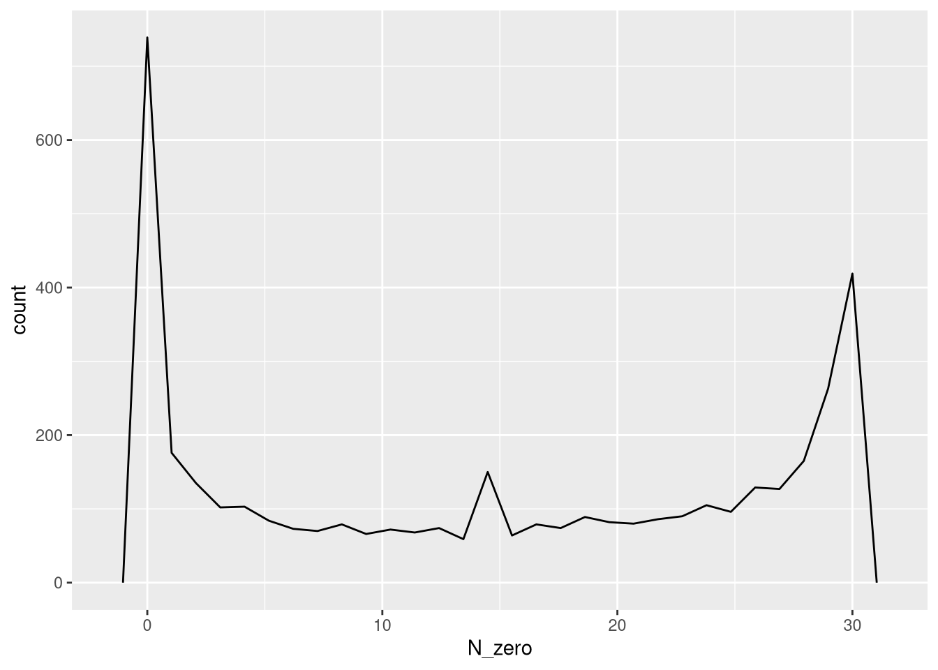
| Version | Author | Date |
|---|---|---|
| 4226c0f | FeiLiyang | 2026-01-07 |
## plot the number of absence for each selected barcode by filtering.
ggplot(data.frame(N_zero = rowSums(detection[mixture_plus1@elementMetadata$isTopBarcode$isTop,] <= 0, na.rm = T))) +
  geom_freqpoly(aes(x = N_zero))
`stat_bin()` using `bins = 30`. Pick better value `binwidth`.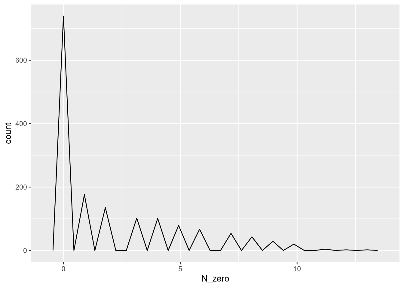
| Version | Author | Date |
|---|---|---|
| 4226c0f | FeiLiyang | 2026-01-07 |
## update the "occurrence" assay based on the detection here.
mixture_plus1@assays@data$occurrence <- detection <= 0
Barcode detection in the two premix samples.
8 Detect correlating barcodes
8.1 FS1D: pairwise correlation
No correlating barcodes detected.Actually,
plotBarcodePairCorrelation(barbieQ = mixture_plus1[rowData(mixture_plus1)$isTopBarcode$isTop,], transformation = "none") +
  theme(legend.position = "top") +
  labs(title = "Mixture data") -> fs1d
processing Barcode pairwise pearson correlation on propotion (none transformation).fs1d Warning: The dot-dot notation (`..y..`) was deprecated in ggplot2 3.4.0.
ℹ Please use `after_stat(y)` instead.
ℹ The deprecated feature was likely used in the barbieQ package.
Please report the issue at <https://github.com/Oshlack/barbieQ>.
This warning is displayed once every 8 hours.
Call `lifecycle::last_lifecycle_warnings()` to see where this warning was
generated.Warning: Removed 2 rows containing missing values or values outside the scale range
(`geom_bar()`).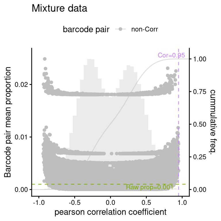
| Version | Author | Date |
|---|---|---|
| 4226c0f | FeiLiyang | 2026-01-07 |
- looking weird if using “asin-sqrt” transformation here.
clusterCorrelatingBarcodes(barbieQ = mixture_plus1[rowData(mixture_plus1)$isTopBarcode$isTop,], transformation = "asin-sqrt") %>%
  inspectCorrelatingBarcodes()
processing Barcode pairwise pearson correlation on propotion (asin-sqrt transformation).identified 3 clusters, including 32 Barcodes.$p_cluster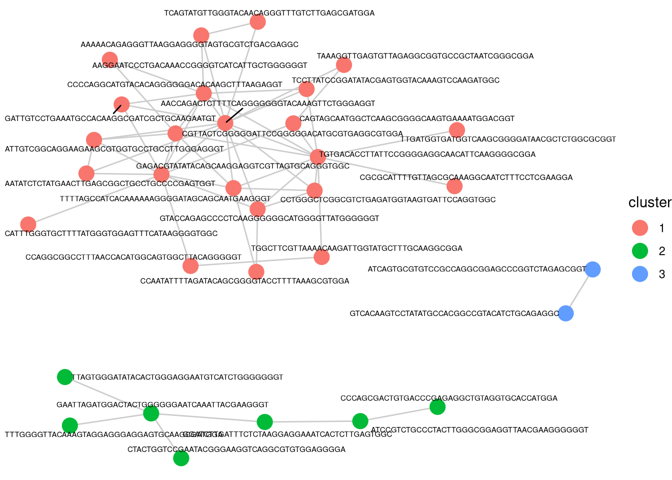
| Version | Author | Date |
|---|---|---|
| 4226c0f | FeiLiyang | 2026-01-07 |
$p_cluster_size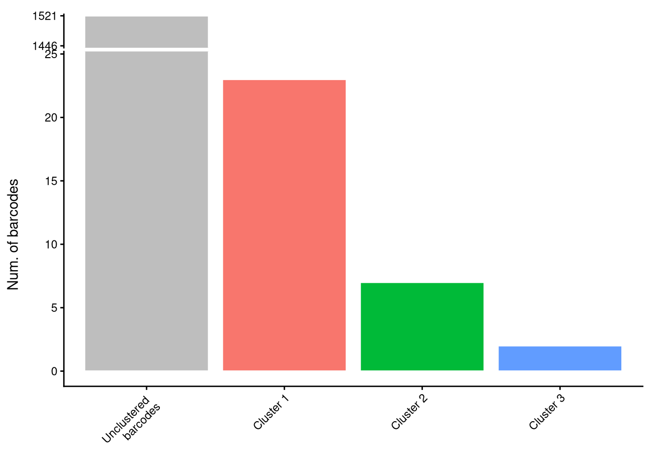
| Version | Author | Date |
|---|---|---|
| 4226c0f | FeiLiyang | 2026-01-07 |
$p_cluster_prop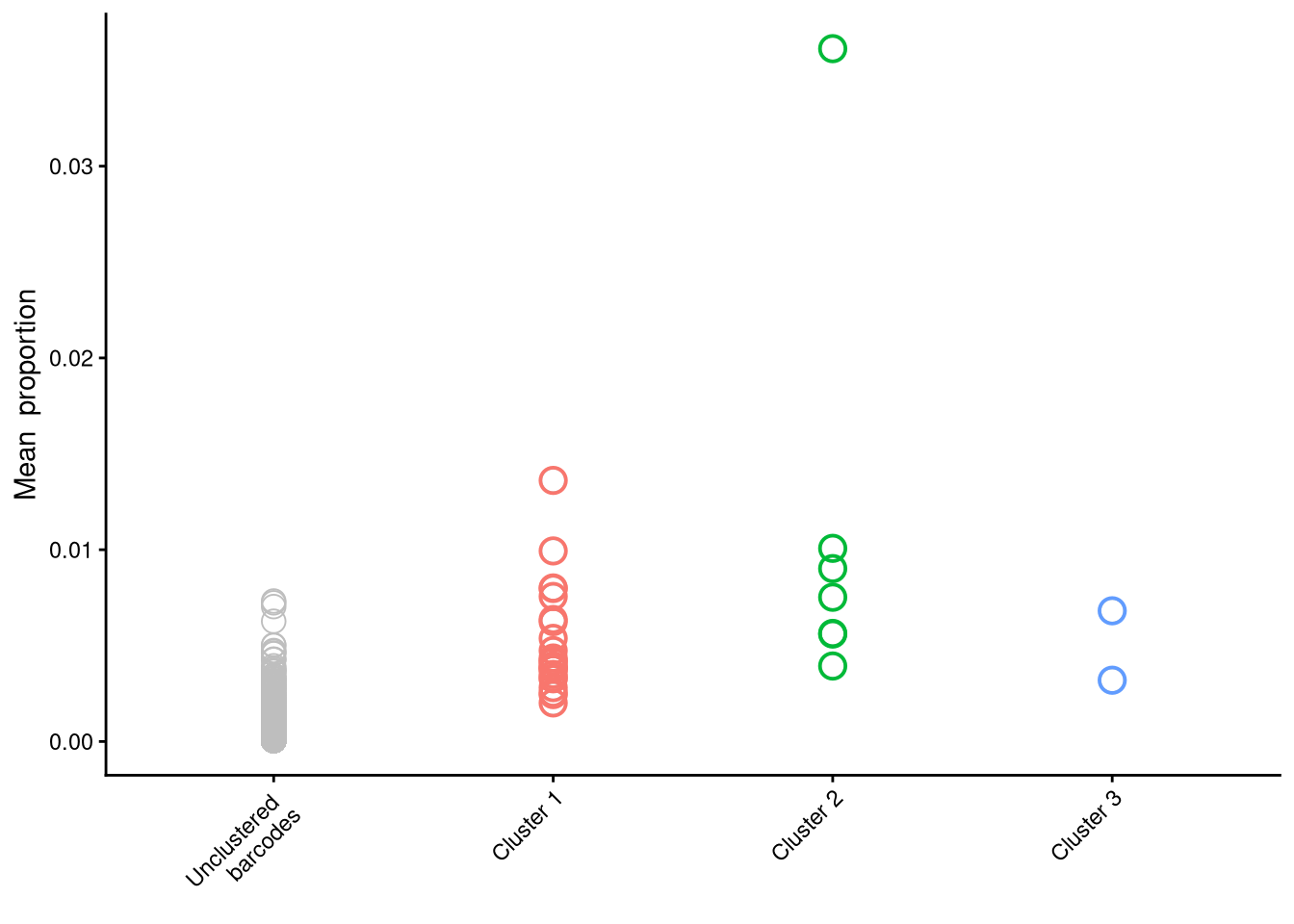
| Version | Author | Date |
|---|---|---|
| 4226c0f | FeiLiyang | 2026-01-07 |
9 Filter top barcodes
9.1 FS1I,L: inspect top/bottom
plotBarcodePareto(mixture_plus1) +
  ylim(-8, 7) +
  annotate("text", x = c(pi * 0.05), y = c(7),
           label = c("Relative proportion %"), color = "#999966",
           size = 3, angle = 0, fontface = "bold", hjust = 1) -> fs1i
Scale for y is already present.
Adding another scale for y, which will replace the existing scale.fs1iWarning: Removed 10 rows containing missing values or values outside the scale range
(`geom_bar()`).Warning: Removed 1 row containing missing values or values outside the scale range
(`geom_segment()`).
Removed 1 row containing missing values or values outside the scale range
(`geom_segment()`).
Removed 1 row containing missing values or values outside the scale range
(`geom_segment()`).Warning: Removed 4 rows containing missing values or values outside the scale range
(`geom_text()`).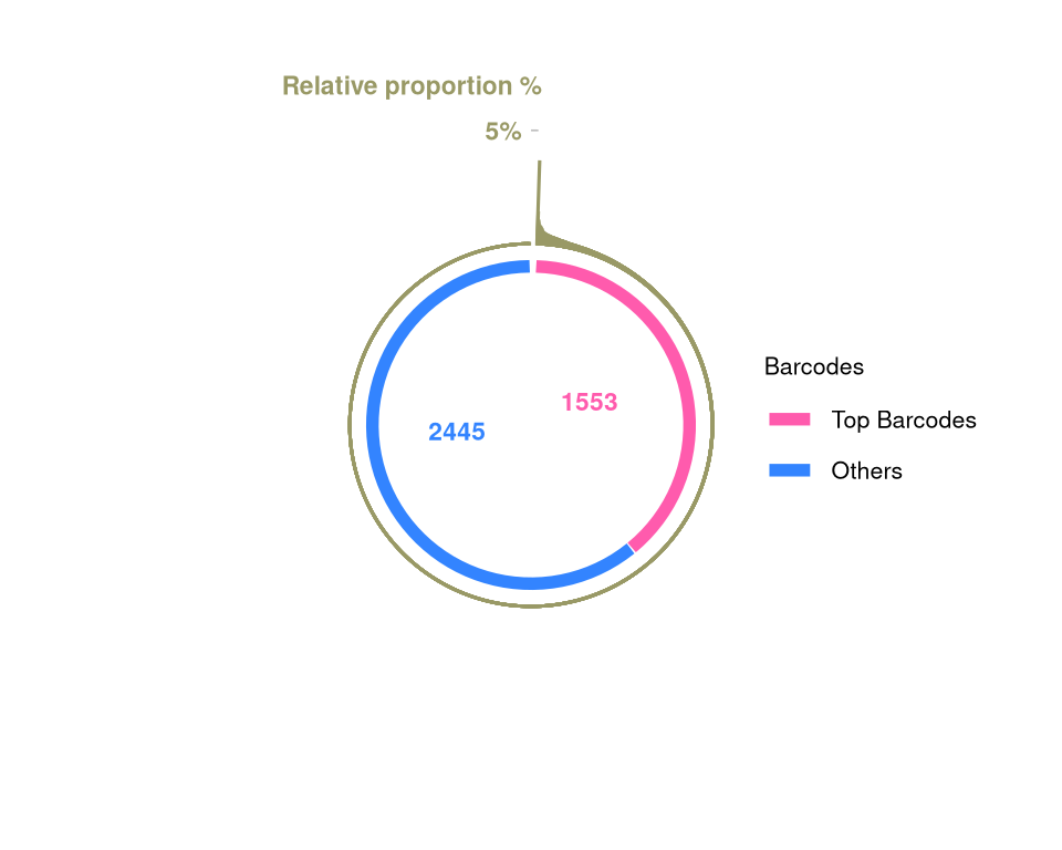
| Version | Author | Date |
|---|---|---|
| 4226c0f | FeiLiyang | 2026-01-07 |
plotBarcodeSankey(mixture_plus1) +
  theme(legend.position = "top") -> fs1l

fs1l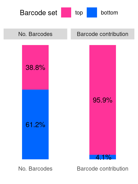
| Version | Author | Date |
|---|---|---|
| 4226c0f | FeiLiyang | 2026-01-07 |
9.2 Filter “top” barcodes
mixture_plus1_top <- mixture_plus1[rowData(mixture_plus1)$isTopBarcode$isTop,]9.3 Heatmap
## pre-filtering
Heatmap(name = "asin-sqrt prop.",
  matrix = asin(sqrt(assays(mixture_plus1)$proportion)),
  row_title = paste0(nrow(mixture_plus1), " Barcodes"),
  show_row_names = FALSE, show_column_names = FALSE)
The automatically generated colors map from the 1^st and 99^th of the
values in the matrix. There are outliers in the matrix whose patterns
might be hidden by this color mapping. You can manually set the color
to `col` argument.
Use `suppressMessages()` to turn off this message.`use_raster` is automatically set to TRUE for a matrix with more than
2000 rows. You can control `use_raster` argument by explicitly setting
TRUE/FALSE to it.
Set `ht_opt$message = FALSE` to turn off this message.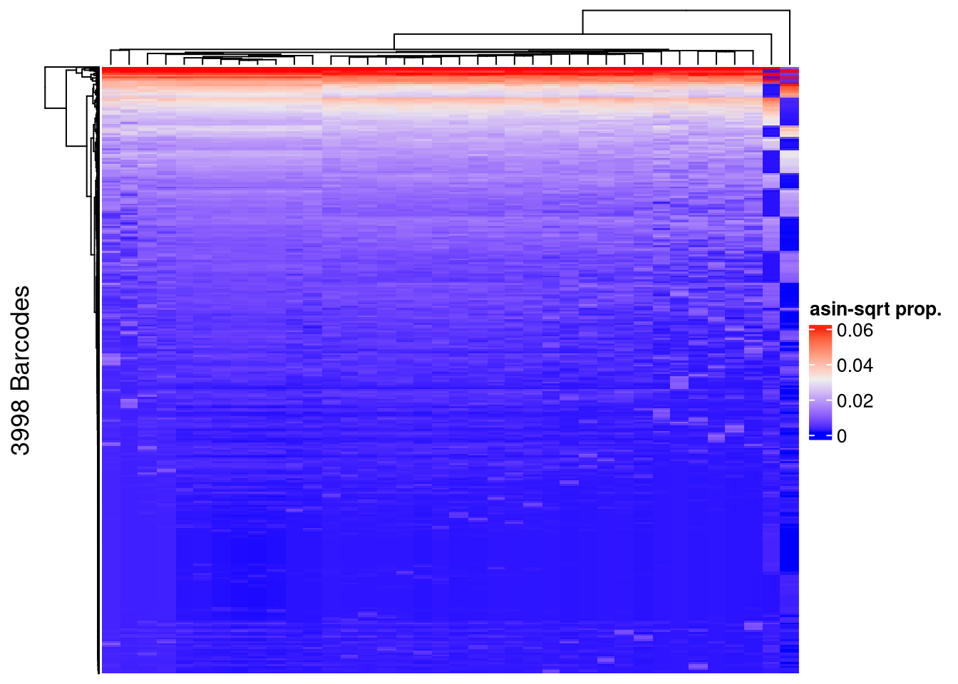
| Version | Author | Date |
|---|---|---|
| 4226c0f | FeiLiyang | 2026-01-07 |
## post-filtering
Heatmap(name = "asin-sqrt prop.",
  matrix = asin(sqrt(assays(mixture_plus1_top)$proportion)),
  row_title = paste0(nrow(mixture_plus1_top), " Barcodes"),
  show_row_names = FALSE, show_column_names = FALSE)
The automatically generated colors map from the 1^st and 99^th of the
values in the matrix. There are outliers in the matrix whose patterns
might be hidden by this color mapping. You can manually set the color
to `col` argument.
Use `suppressMessages()` to turn off this message.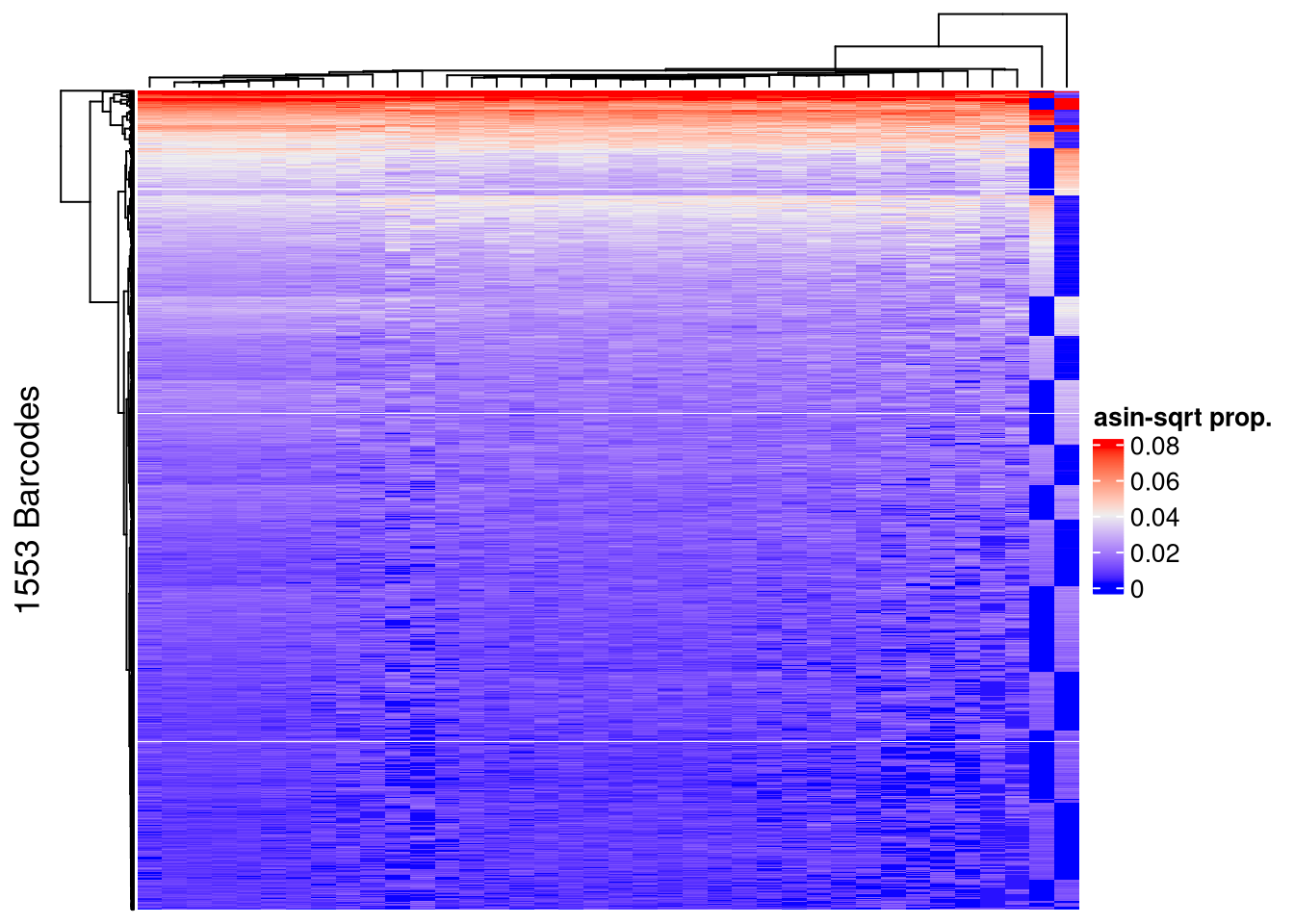
| Version | Author | Date |
|---|---|---|
| 4226c0f | FeiLiyang | 2026-01-07 |
10 Save to rda
save(mixture_plus1, mixture_plus1_top, file = "output/mixture_barbieQ.rda")11 FigureS1-Mixture
layout = "
DDDD
####
IIII
LLLL
"
fs1_mixture <- (
  wrap_elements(fs1d + theme(plot.margin = unit(c(0,0,0,0), "line"))) +
    wrap_elements(fs1i + theme(plot.margin = unit(rep(0,4), "cm"))) +
    wrap_elements(fs1l + theme(plot.margin = unit(rep(0,4), "cm")))
  ) +
  plot_layout(design = layout) +
  plot_annotation(tag_levels = list(c("D"," ", "I","L"))) &
  theme(
    plot.tag = element_text(size = 20, face = "bold", family = "arial"),
    axis.title = element_text(size = 17),
    axis.text = element_text(size = 12),
    legend.title = element_text(size = 13),
    legend.text = element_text(size = 11))

fs1_mixture
Warning: Removed 2 rows containing missing values or values outside the scale range
(`geom_bar()`).Warning: Removed 10 rows containing missing values or values outside the scale range
(`geom_bar()`).Warning: Removed 1 row containing missing values or values outside the scale range
(`geom_segment()`).
Removed 1 row containing missing values or values outside the scale range
(`geom_segment()`).
Removed 1 row containing missing values or values outside the scale range
(`geom_segment()`).Warning: Removed 4 rows containing missing values or values outside the scale range
(`geom_text()`).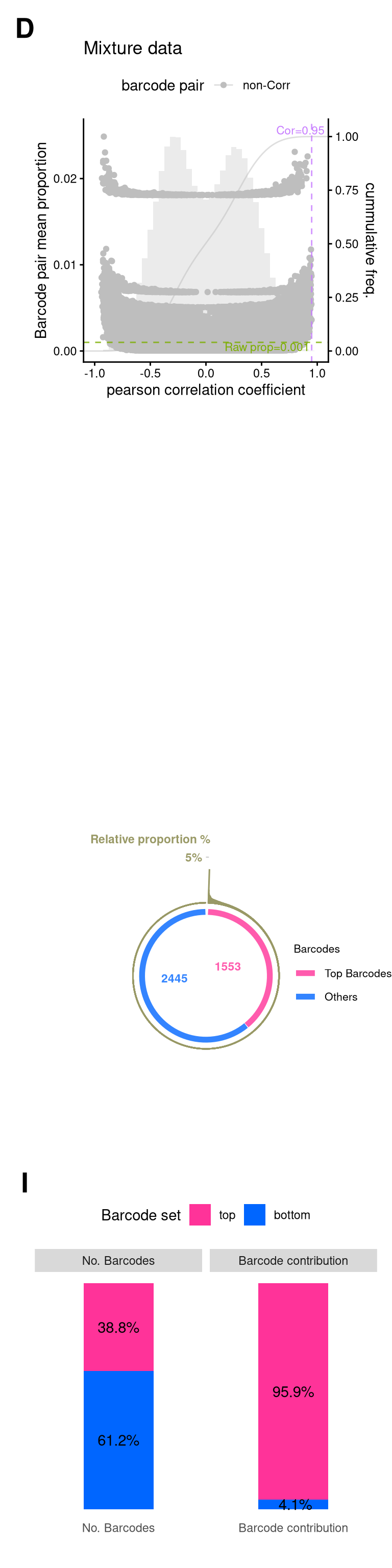
| Version | Author | Date |
|---|---|---|
| 4226c0f | FeiLiyang | 2026-01-07 |
ggsave(
  filename = "output/fs1_mixture.png",
  plot = fs1_mixture,
  width = 4,
  height = 16,
  units = "in", # for Rmd r chunk fig size, unit default to inch
  dpi = 350
  )
Warning: Removed 2 rows containing missing values or values outside the scale range
(`geom_bar()`).Warning: Removed 10 rows containing missing values or values outside the scale range
(`geom_bar()`).Warning: Removed 1 row containing missing values or values outside the scale range
(`geom_segment()`).
Removed 1 row containing missing values or values outside the scale range
(`geom_segment()`).
Removed 1 row containing missing values or values outside the scale range
(`geom_segment()`).Warning: Removed 4 rows containing missing values or values outside the scale range
(`geom_text()`).Saving this figure in fs1_mixture
sessionInfo()R version 4.5.0 (2025-04-11)
Platform: x86_64-pc-linux-gnu
Running under: Red Hat Enterprise Linux 9.6 (Plow)
Matrix products: default
BLAS/LAPACK: FlexiBLAS OPENBLAS-OPENMP; LAPACK version 3.9.0
locale:
[1] LC_CTYPE=en_AU.UTF-8 LC_NUMERIC=C
[3] LC_TIME=en_AU.UTF-8 LC_COLLATE=en_AU.UTF-8
[5] LC_MONETARY=en_AU.UTF-8 LC_MESSAGES=en_AU.UTF-8
[7] LC_PAPER=en_AU.UTF-8 LC_NAME=C
[9] LC_ADDRESS=C LC_TELEPHONE=C
[11] LC_MEASUREMENT=en_AU.UTF-8 LC_IDENTIFICATION=C
time zone: Australia/Melbourne
tzcode source: system (glibc)
attached base packages:
[1] grid stats4 stats graphics grDevices utils datasets
[8] methods base
other attached packages:
[1] barbieQ_1.1.3 edgeR_4.6.3
[3] limma_3.64.3 eulerr_7.0.4
[5] magick_2.9.0 ComplexHeatmap_2.24.1
[7] ggVennDiagram_1.5.4 scales_1.4.0
[9] patchwork_1.3.2 ggnewscale_0.5.2
[11] ggbreak_0.1.6 ggplot2_4.0.0
[13] SummarizedExperiment_1.38.1 Biobase_2.68.0
[15] GenomicRanges_1.60.0 GenomeInfoDb_1.44.3
[17] IRanges_2.42.0 S4Vectors_0.48.0
[19] BiocGenerics_0.54.0 generics_0.1.4
[21] MatrixGenerics_1.20.0 matrixStats_1.5.0
[23] data.table_1.17.8 knitr_1.50
[25] tibble_3.3.0 tidyr_1.3.1
[27] dplyr_1.1.4 magrittr_2.0.4
[29] readxl_1.4.5 workflowr_1.7.2
loaded via a namespace (and not attached):
[1] RColorBrewer_1.1-3 rstudioapi_0.17.1 jsonlite_2.0.0
[4] shape_1.4.6.1 jomo_2.7-6 nloptr_2.2.1
[7] farver_2.1.2 logistf_1.26.1 rmarkdown_2.30
[10] ragg_1.5.0 GlobalOptions_0.1.2 fs_1.6.6
[13] vctrs_0.6.5 minqa_1.2.8 memoise_2.0.1
[16] htmltools_0.5.8.1 S4Arrays_1.8.1 broom_1.0.10
[19] cellranger_1.1.0 SparseArray_1.8.1 gridGraphics_0.5-1
[22] mitml_0.4-5 sass_0.4.10 bslib_0.9.0
[25] cachem_1.1.0 whisker_0.4.1 igraph_2.1.4
[28] lifecycle_1.0.4 iterators_1.0.14 pkgconfig_2.0.3
[31] Matrix_1.7-3 R6_2.6.1 fastmap_1.2.0
[34] rbibutils_2.3 GenomeInfoDbData_1.2.14 clue_0.3-66
[37] digest_0.6.37 aplot_0.2.9 colorspace_2.1-2
[40] ps_1.9.1 rprojroot_2.1.1 textshaping_1.0.3
[43] labeling_0.4.3 httr_1.4.7 polyclip_1.10-7
[46] abind_1.4-8 mgcv_1.9-1 compiler_4.5.0
[49] withr_3.0.2 doParallel_1.0.17 backports_1.5.0
[52] S7_0.2.0 viridis_0.6.5 ggforce_0.5.0
[55] pan_1.9 MASS_7.3-65 rappdirs_0.3.3
[58] DelayedArray_0.34.1 rjson_0.2.23 tools_4.5.0
[61] httpuv_1.6.16 nnet_7.3-20 glue_1.8.0
[64] callr_3.7.6 nlme_3.1-168 promises_1.3.3
[67] getPass_0.2-4 cluster_2.1.8.1 operator.tools_1.6.3
[70] gtable_0.3.6 formula.tools_1.7.1 tidygraph_1.3.1
[73] XVector_0.48.0 ggrepel_0.9.6 foreach_1.5.2
[76] pillar_1.11.1 stringr_1.5.2 yulab.utils_0.2.1
[79] later_1.4.4 circlize_0.4.16 splines_4.5.0
[82] tweenr_2.0.3 lattice_0.22-6 survival_3.8-3
[85] tidyselect_1.2.1 locfit_1.5-9.12 git2r_0.36.2
[88] reformulas_0.4.1 gridExtra_2.3 xfun_0.53
[91] graphlayouts_1.2.2 statmod_1.5.0 stringi_1.8.7
[94] UCSC.utils_1.4.0 boot_1.3-31 ggfun_0.2.0
[97] yaml_2.3.10 evaluate_1.0.5 codetools_0.2-20
[100] ggraph_2.2.2 ggplotify_0.1.3 cli_3.6.5
[103] rpart_4.1.24 systemfonts_1.3.1 Rdpack_2.6.4
[106] processx_3.8.6 jquerylib_0.1.4 Rcpp_1.1.0
[109] png_0.1-8 parallel_4.5.0 lme4_1.1-37
[112] glmnet_4.1-10 viridisLite_0.4.2 purrr_1.1.0
[115] crayon_1.5.3 GetoptLong_1.0.5 rlang_1.1.6
[118] mice_3.18.0