Last updated: 2026-01-07

Checks: 5 2

Knit directory: public_barcode_count/

This reproducible R Markdown analysis was created with workflowr (version 1.7.2). The Checks tab describes the reproducibility checks that were applied when the results were created. The Past versions tab lists the development history.

R Markdown file: uncommitted changes

The R Markdown is untracked by Git. To know which version of the R Markdown file created these results, you’ll want to first commit it to the Git repo. If you’re still working on the analysis, you can ignore this warning. When you’re finished, you can run wflow_publish to commit the R Markdown file and build the HTML.

Environment: objects present

The global environment had objects present when the code in the R Markdown file was run. These objects can affect the analysis in your R Markdown file in unknown ways. For reproduciblity it’s best to always run the code in an empty environment. Use wflow_publish or wflow_build to ensure that the code is always run in an empty environment.

The following objects were defined in the global environment when these results were created:

Name	Class	Size
module	function	5.6 Kb

Seed: set.seed(20250112)

The command set.seed(20250112) was run prior to running the code in the R Markdown file. Setting a seed ensures that any results that rely on randomness, e.g. subsampling or permutations, are reproducible.

Session information: recorded

Great job! Recording the operating system, R version, and package versions is critical for reproducibility.

Cache: none

Nice! There were no cached chunks for this analysis, so you can be confident that you successfully produced the results during this run.

File paths: relative

Great job! Using relative paths to the files within your workflowr project makes it easier to run your code on other machines.

Repository version: 34f5894

Great! You are using Git for version control. Tracking code development and connecting the code version to the results is critical for reproducibility.

The results in this page were generated with repository version 34f5894. See the Past versions tab to see a history of the changes made to the R Markdown and HTML files.

Note that you need to be careful to ensure that all relevant files for the analysis have been committed to Git prior to generating the results (you can use wflow_publish or wflow_git_commit). workflowr only checks the R Markdown file, but you know if there are other scripts or data files that it depends on. Below is the status of the Git repository when the results were generated:


Ignored files:
    Ignored:    .RData
    Ignored:    .Rhistory
    Ignored:    .Rproj.user/
    Ignored:    public_barcode_count.Rproj

Untracked files:
    Untracked:  analysis/barbieQ_paper_FigureS1_AML.Rmd
    Untracked:  analysis/barbieQ_paper_FigureS1_Mixture.Rmd
    Untracked:  analysis/barbieQ_paper_FigureS1_xenoHSPC.Rmd
    Untracked:  analysis/barbieQ_paper_FigureS2_AML.Rmd
    Untracked:  analysis/barbieQ_paper_FigureS2_xenoHSPC.Rmd
    Untracked:  output/AML_barbieQ.rda
    Untracked:  output/AML_negative_simulation.rda
    Untracked:  output/fs1_aml.png
    Untracked:  output/fs1_mixture.png
    Untracked:  output/fs1_xeno.png
    Untracked:  output/fs1a_knowncluster.png
    Untracked:  output/fs2_aml.png
    Untracked:  output/fs2_xeno.png
    Untracked:  output/xenoC21_negative_simulation.rda
    Untracked:  output/xenoC22_negative_simulation.rda
    Untracked:  output/xenoC23_negative_simulation.rda
    Untracked:  output/xenoHSPC_barbieQ.rda

Unstaged changes:
    Modified:   analysis/F3_simulation.R
    Modified:   analysis/barbieQ_paper_Figure2.Rmd
    Deleted:    analysis/barbieQ_paper_S1.Rmd
    Modified:   analysis/index.Rmd
    Modified:   data/BelderbosME/README.md
    Modified:   output/f2.png
    Modified:   output/monkeyHSPC_barbieQ.rda
    Modified:   output/monkeyHSPC_raw_barbieQ.rda

Note that any generated files, e.g. HTML, png, CSS, etc., are not included in this status report because it is ok for generated content to have uncommitted changes.

There are no past versions. Publish this analysis with wflow_publish() to start tracking its development.

Links to Type I error rate assessment using other datasets in the barbieQ paper:

1 Load Dependencies

library(readxl)
library(magrittr)
library(dplyr)
library(tidyr) # for pivot_longer
library(tibble) # for rownames_to _column
library(knitr) # for kable()
library(ggplot2)
library(patchwork)
library(scales)
library(ggVennDiagram)
library(ComplexHeatmap)
library(limma)
library(edgeR)
library(SummarizedExperiment)
library(SEtools)
library(S4Vectors)
library(devtools)
# devtools::install_github("DaneVass/bartools", dependencies = TRUE, force = TRUE)
# library(bartools)

source("analysis/plotBarcodeHistogram.R") ## accommodated from bartools::plotBarcodehistogram
source("analysis/F3_simulation.R") ## for negative simulation
source("analysis/ggplot_theme.R") ## setting ggplot theme

2 Install `barbieQ`

Installing the latest devel version of barbieQ from GitHub.

if (!requireNamespace("barbieQ", quietly = TRUE)) {
  remotes::install_github("Oshlack/barbieQ")
}

Warning: replacing previous import 'data.table::first' by 'dplyr::first' when
loading 'barbieQ'

Warning: replacing previous import 'data.table::last' by 'dplyr::last' when
loading 'barbieQ'

Warning: replacing previous import 'data.table::between' by 'dplyr::between'
when loading 'barbieQ'

Warning: replacing previous import 'dplyr::as_data_frame' by
'igraph::as_data_frame' when loading 'barbieQ'

Warning: replacing previous import 'dplyr::groups' by 'igraph::groups' when
loading 'barbieQ'

Warning: replacing previous import 'dplyr::union' by 'igraph::union' when
loading 'barbieQ'

Registered S3 method overwritten by 'formula.tools':
  method               from    
  as.character.formula openxlsx

library(barbieQ)

Check the version of barbieQ.

packageVersion("barbieQ")

[1] '1.1.3'

3 Set seeds

set.seed(2025)

4 Load preprocessed data

Links to AML data preprocessing

load("output/AML_barbieQ.rda")

5 Samples level QC

5.1 PCA

pca_results <- (assays(AML_top)$proportion) %>% sqrt() %>% asin() %>% 
  t() %>% 
  prcomp()

var_pct <- pca_results$sdev^2 / sum(pca_results$sdev^2) * 100
var_pct

 [1] 4.076279e+01 2.507797e+01 1.531253e+01 5.537856e+00 3.346360e+00
 [6] 2.044106e+00 1.625127e+00 1.106829e+00 7.862013e-01 7.028069e-01
[11] 6.121548e-01 5.392358e-01 3.813225e-01 2.848237e-01 2.636818e-01
[16] 2.415583e-01 2.224249e-01 1.783012e-01 1.293819e-01 1.141377e-01
[21] 9.559165e-02 8.685013e-02 7.950005e-02 6.285928e-02 5.813735e-02
[26] 4.994494e-02 4.071874e-02 3.821716e-02 3.269847e-02 2.767458e-02
[31] 2.619478e-02 2.492990e-02 2.221603e-02 2.060769e-02 1.861592e-02
[36] 1.411699e-02 1.063725e-02 8.653785e-03 7.951038e-03 4.283570e-03
[41] 8.039042e-30

pca_df <- data.frame(
  PC1 = pca_results$x[, 1],
  PC2 = pca_results$x[, 2],
  AML_top$sampleMetadata
)

ggplot(pca_df, aes(x = PC1, y = PC2, color = Treatment)) +
  geom_point(size = 3) +
  labs(title = "PCA on asin-sqrt prop.", 
       x = paste0("PC1 (", round(var_pct[1], 2), " %)"), 
       y = paste0("PC2 (", round(var_pct[2], 2), " %)")) +
  theme_classic() +
  theme(aspect.ratio = 1)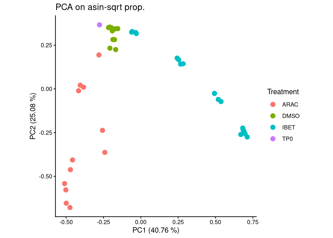

ggplot(pca_df, aes(x = PC1, y = PC2, color = Dose)) +
  geom_point(size = 3) +
  labs(title = "PCA on asin-sqrt prop.", 
       x = paste0("PC1 (", round(var_pct[1], 2), " %)"), 
       y = paste0("PC2 (", round(var_pct[2], 2), " %)")) +
  theme_classic() +
  theme(aspect.ratio = 1)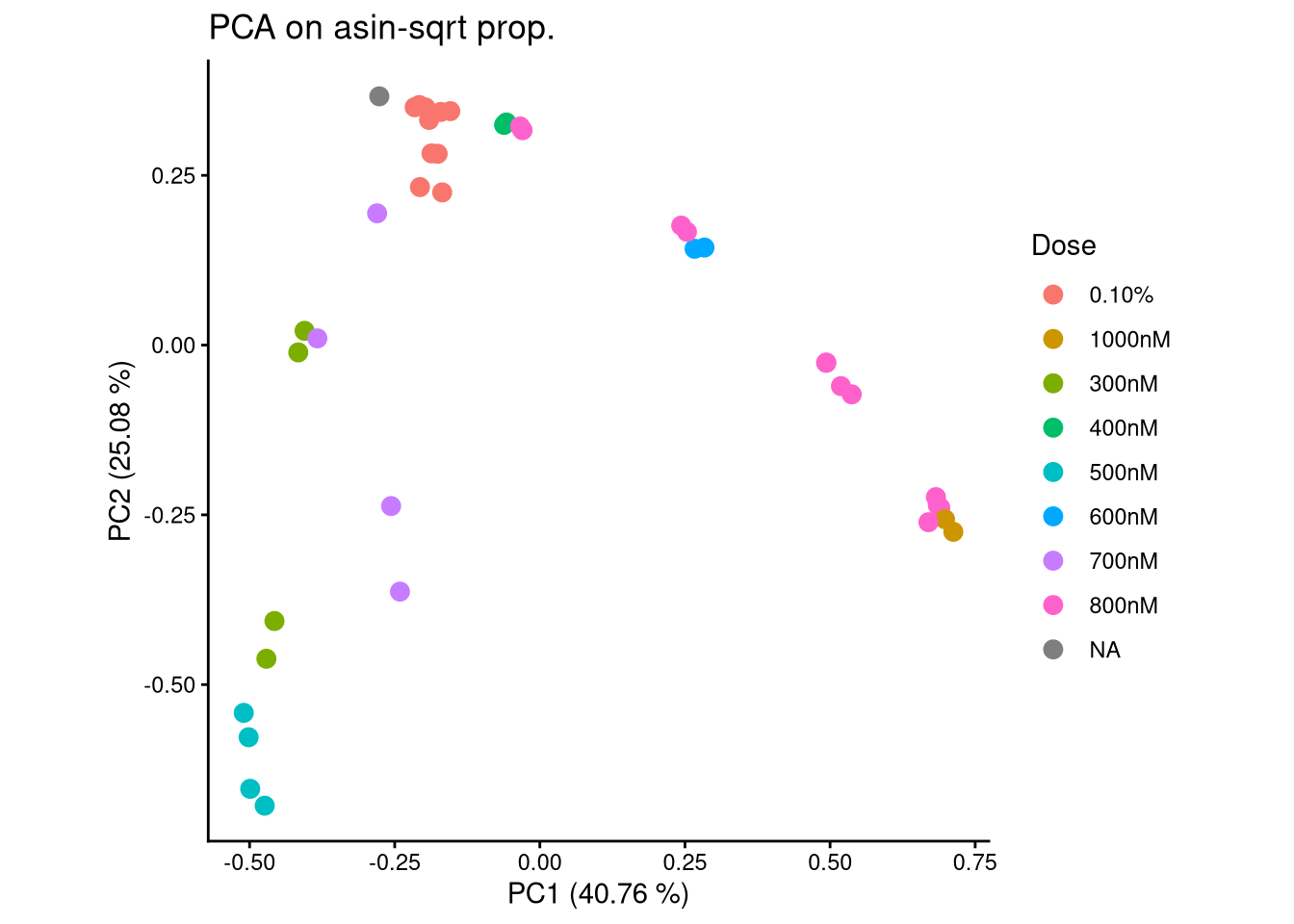

ggplot(pca_df, aes(x = PC1, y = PC2, color = Timepoint)) +
  geom_point(size = 3) +
  labs(title = "PCA on asin-sqrt prop.", 
       x = paste0("PC1 (", round(var_pct[1], 2), " %)"), 
       y = paste0("PC2 (", round(var_pct[2], 2), " %)")) +
  theme_classic() +
  theme(aspect.ratio = 1)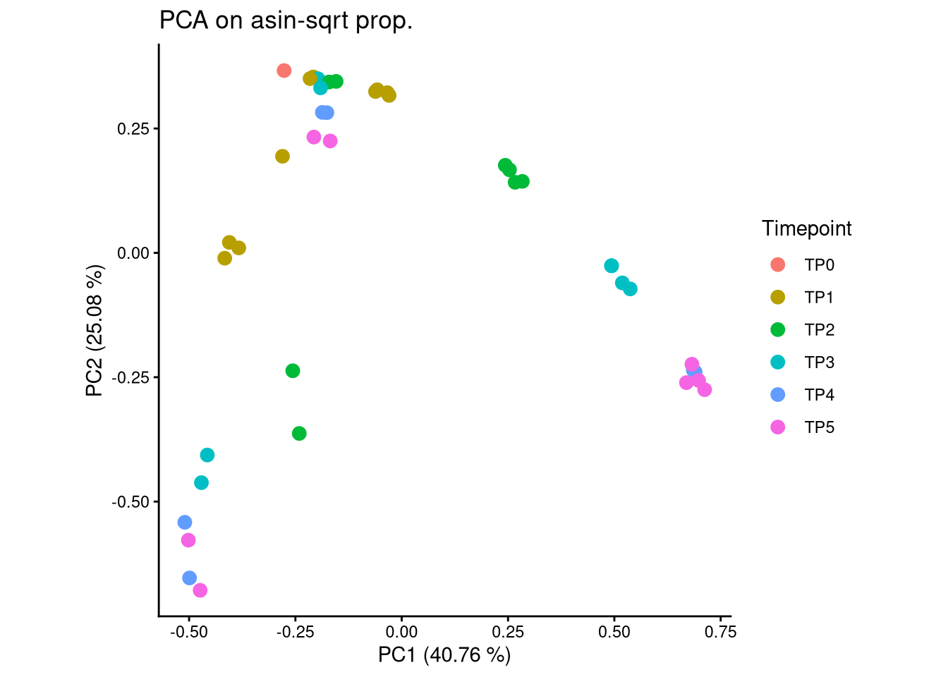

5.2 Plot propportion

## order samples
order_sample <- AML_top$sampleMetadata %>% with(order(Treatment, Dose, Timepoint))

## create bartools object
AML_dge <- DGEList(
  counts = assay(AML_top), 
  group = AML_top$sampleMetadata$Treatment)

## plot 
plotBarcodeHistogram(AML_dge, orderSamples = colnames(AML_top)[order_sample])

Warning: Use of .data in tidyselect expressions was deprecated in tidyselect 1.2.0.
ℹ Please use `"barcode"` instead of `.data$barcode`
This warning is displayed once every 8 hours.
Call `lifecycle::last_lifecycle_warnings()` to see where this warning was
generated.

Warning: Use of .data in tidyselect expressions was deprecated in tidyselect 1.2.0.
ℹ Please use `"value"` instead of `.data$value`
This warning is displayed once every 8 hours.
Call `lifecycle::last_lifecycle_warnings()` to see where this warning was
generated.

Warning: Use of .data in tidyselect expressions was deprecated in tidyselect 1.2.0.
ℹ Please use `"name"` instead of `.data$name`
This warning is displayed once every 8 hours.
Call `lifecycle::last_lifecycle_warnings()` to see where this warning was
generated.

Warning: Use of .data in tidyselect expressions was deprecated in tidyselect 1.2.0.
ℹ Please use `"freq"` instead of `.data$freq`
This warning is displayed once every 8 hours.
Call `lifecycle::last_lifecycle_warnings()` to see where this warning was
generated.

Warning: The `guide` argument in `scale_*()` cannot be `FALSE`. This was deprecated in
ggplot2 3.3.4.
ℹ Please use "none" instead.
This warning is displayed once every 8 hours.
Call `lifecycle::last_lifecycle_warnings()` to see where this warning was
generated.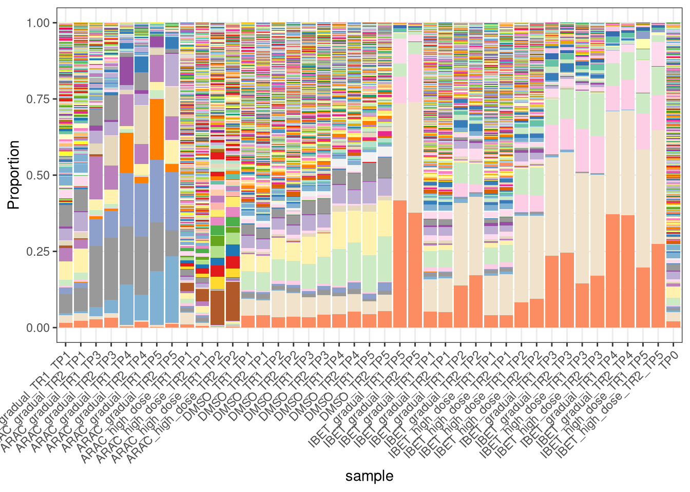

5.3 Subet DMSO

DMSO <- AML_top[, AML_top$sampleMetadata$Treatment == "DMSO"]

pca_results <- (assays(DMSO)$proportion) %>% sqrt() %>% asin() %>% 
  t() %>% 
  prcomp()

var_pct <- pca_results$sdev^2 / sum(pca_results$sdev^2) * 100
var_pct

 [1] 7.752146e+01 9.395912e+00 4.157909e+00 3.336706e+00 2.553178e+00
 [6] 1.079995e+00 8.330679e-01 7.617977e-01 3.599713e-01 4.692581e-30

pca_dmso <- data.frame(
  PC1 = pca_results$x[, 1],
  PC2 = pca_results$x[, 2],
  DMSO$sampleMetadata
)

ggplot(pca_dmso, aes(x = PC1, y = PC2, color = Timepoint)) +
  geom_point(size = 3) +
  labs(title = "PCA on asin-sqrt prop.", 
       x = paste0("PC1 (", round(var_pct[1], 2), " %)"), 
       y = paste0("PC2 (", round(var_pct[2], 2), " %)")) +
  theme_classic() +
  theme(aspect.ratio = 1)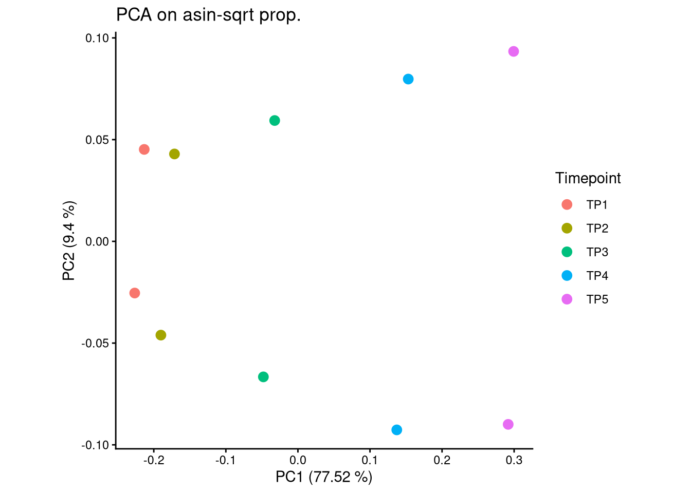

5.4 FS2G: prop. DMSO

## order samples
order_sample <- DMSO$sampleMetadata %>% with(order(Timepoint))

## create bartools object
DMSO_dge <- DGEList(
  counts = assay(DMSO), 
  group = DMSO$sampleMetadata$Timepoint)

## plot 
plotBarcodeHistogram(DMSO_dge, orderSamples = colnames(DMSO)[order_sample]) + 
  labs(title = "AML: DMSO") -> p_prop_DMSO

p_prop_DMSO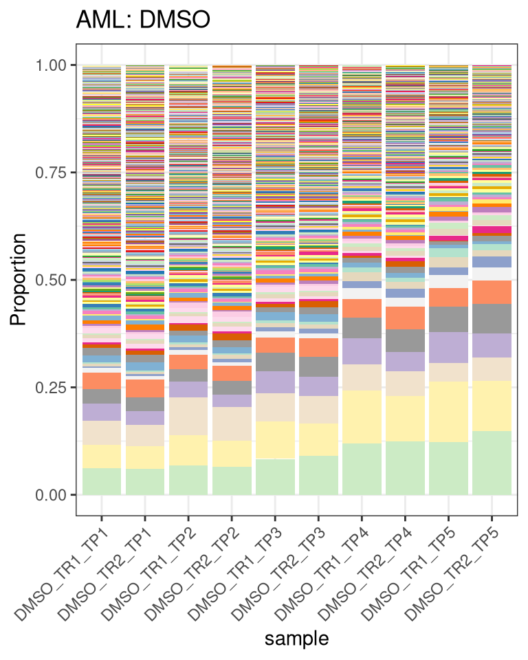

6 Type I error rate

6.1 Negative simulation

avoid running this chunk during rendering. global_all_loops was saved from the first run.

results_negsi <- suppressMessages({
  random_sampling(barbieQ = DMSO, loop_times = 100)
  })

## `random_sampling()` save the simulations to global environment as `global_all_loops`
save(global_all_loops, file = "output/AML_negative_simulation.rda")

load results

## loading random sampling results to avoid running it repeatedly
load("output/AML_negative_simulation.rda")

# extract results from the loops
end_sampling <- floor(ncol(DMSO)/2)

## extract FPR
all_FPR <- lapply(seq(3:end_sampling), function(n) {
  global_all_loops[[n]]$FPR
})
df_FPR_DMSO <- do.call(rbind, all_FPR)

plot FPR

df_FPR_DMSO$N_Samples <- as.factor(df_FPR_DMSO$N_Samples)

## Diff_Prop
## reshape the data to fit methods for testing
df_FPR_DMSO_long <- df_FPR_DMSO %>%
  pivot_longer(cols = starts_with("Prop_"),
               names_to = "Method",
               values_to = "Pval_Prop") %>%
  mutate(Method = factor(Method, levels = c("Prop_asin", "Prop_logit", "Prop_noTrans"),
                         labels = c("asin-sqrt", "logit", "no trans.")))

P_FPR_prop_DMSO <- ggplot(
  df_FPR_DMSO_long, aes(x = factor(N_Samples), y = Pval_Prop, color = Method)) +
  geom_boxplot(outlier.shape = 1, position = position_dodge(width = 0.7)) +
  # geom_jitter(size = 1, position = position_dodge(width = 0.7)) +
  geom_hline(yintercept = 0.05, linetype = "dashed", color = "black") +
  # coord_cartesian(ylim = c(0, 0.2)) + 
  labs(
       y = "Fraction of P-Value < 0.05",
       x = "Number of samples per group",
       # title = "DMSO",
       subtitle = "Differential proportion test") +
  # facet_wrap(~Method, scales = "free_y") +
  theme_classic() +
  theme(legend.position = "top")

## Diff_Occ
P_FPR_occ_DMSO <- ggplot(
  df_FPR_DMSO, aes(x = factor(N_Samples), y = Occ_firth)) +
  geom_boxplot(outlier.shape = 1, position = position_dodge(width = 0.7)) +
  # geom_jitter(size = 1, position = position_dodge(width = 0.7)) +
  geom_hline(yintercept = 0.05, linetype = "dashed", color = "black") +
  scale_color_manual(values = c("Differential occurrrence test" = "black")) +
  # coord_cartesian(ylim = c(0, 0.2)) + 
  labs(
       y = "Fraction of P-Value < 0.05",
       x = "Number of samples per group",
       titlte = "",
       subtitle = "Differential occurrence test") +
  theme_classic() +
  theme(legend.position = "top")

6.2 FS2H: FPR

(P_FPR_prop_DMSO + theme(legend.position = "top")) + (P_FPR_occ_DMSO) -> P_FPR_DMSO

P_FPR_DMSO

Ignoring unknown labels:
• titlte : ""

Warning: No shared levels found between `names(values)` of the manual scale and the
data's colour values.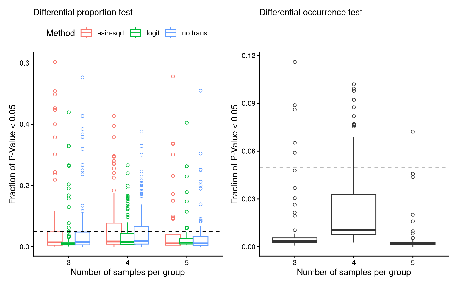

7 Figure S2-AML

layout = "
GHH
"
fs2_aml <- (
    wrap_elements(p_prop_DMSO + theme(plot.margin = unit(c(0,0,0,0), "line"))) + 
  wrap_elements(P_FPR_DMSO + theme(legend.position = "top") + theme(plot.margin = unit(rep(0,4), "cm")))
) + 
  plot_layout(design = layout) +
  plot_annotation(tag_levels = list(c("G", "H"))) &
  theme(
    plot.tag = element_text(size = 20, face = "bold", family = "arial"),
    axis.title = element_text(size = 17),
    axis.text = element_text(size = 12),
    legend.title = element_text(size = 13),
    legend.text = element_text(size = 11))

fs2_aml

Ignoring unknown labels:
• titlte : ""

Warning: No shared levels found between `names(values)` of the manual scale and the
data's colour values.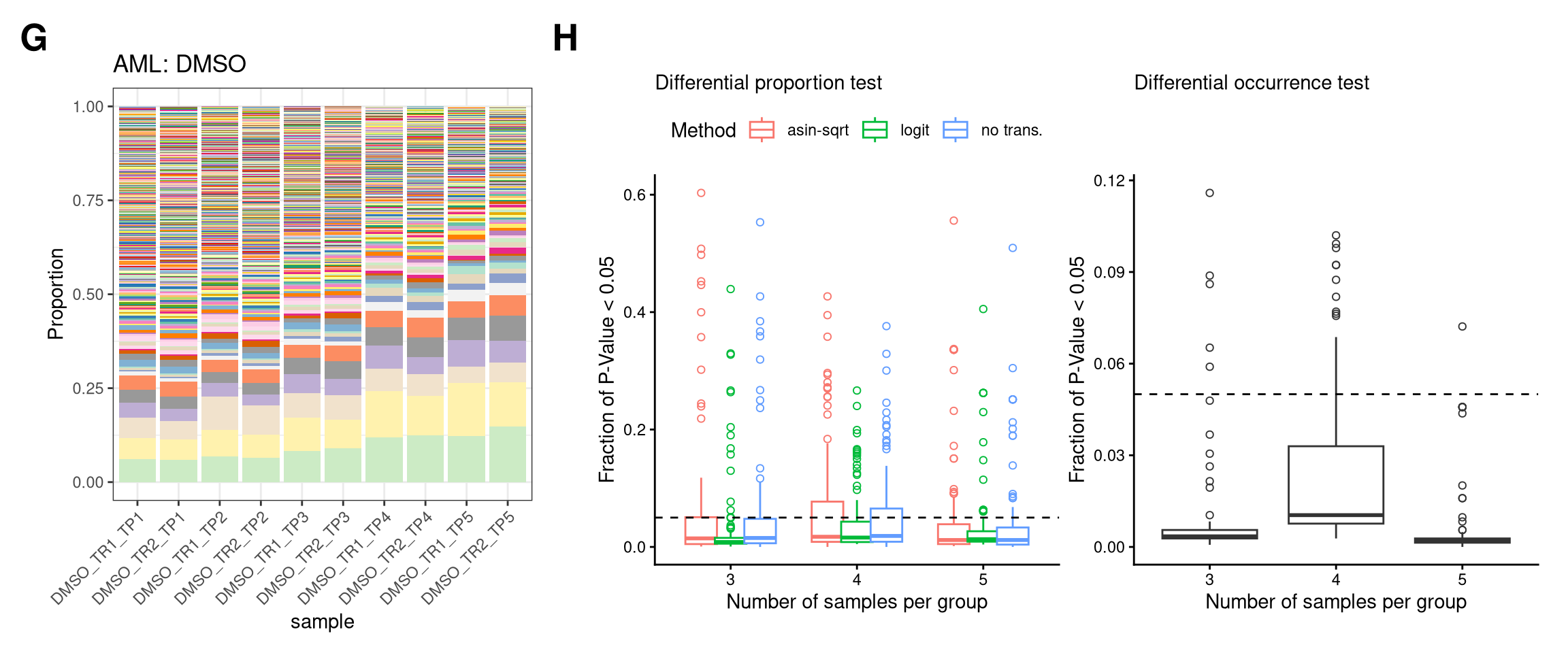

ggsave(
  filename = "output/fs2_aml.png",
  plot = fs2_aml,
  width = 12,
  height = 5,
  units = "in", # for Rmd r chunk fig size, unit default to inch
  dpi = 350
  )

Ignoring unknown labels:
• titlte : ""

Warning: No shared levels found between `names(values)` of the manual scale and the
data's colour values.

Saving this figure in fs2_AML

sessionInfo()

R version 4.5.0 (2025-04-11)
Platform: x86_64-pc-linux-gnu
Running under: Red Hat Enterprise Linux 9.6 (Plow)

Matrix products: default
BLAS/LAPACK: FlexiBLAS OPENBLAS-OPENMP;  LAPACK version 3.9.0

locale:
 [1] LC_CTYPE=en_AU.UTF-8       LC_NUMERIC=C              
 [3] LC_TIME=en_AU.UTF-8        LC_COLLATE=en_AU.UTF-8    
 [5] LC_MONETARY=en_AU.UTF-8    LC_MESSAGES=en_AU.UTF-8   
 [7] LC_PAPER=en_AU.UTF-8       LC_NAME=C                 
 [9] LC_ADDRESS=C               LC_TELEPHONE=C            
[11] LC_MEASUREMENT=en_AU.UTF-8 LC_IDENTIFICATION=C       

time zone: Australia/Melbourne
tzcode source: system (glibc)

attached base packages:
[1] stats4    grid      stats     graphics  grDevices utils     datasets 
[8] methods   base     

other attached packages:
 [1] barbieQ_1.1.3               devtools_2.4.6             
 [3] usethis_3.2.1               SEtools_1.22.0             
 [5] sechm_1.16.0                SummarizedExperiment_1.38.1
 [7] Biobase_2.68.0              GenomicRanges_1.60.0       
 [9] GenomeInfoDb_1.44.3         IRanges_2.42.0             
[11] S4Vectors_0.48.0            BiocGenerics_0.54.0        
[13] generics_0.1.4              MatrixGenerics_1.20.0      
[15] matrixStats_1.5.0           edgeR_4.6.3                
[17] limma_3.64.3                ComplexHeatmap_2.24.1      
[19] ggVennDiagram_1.5.4         scales_1.4.0               
[21] patchwork_1.3.2             ggplot2_4.0.0              
[23] knitr_1.50                  tibble_3.3.0               
[25] tidyr_1.3.1                 dplyr_1.1.4                
[27] magrittr_2.0.4              readxl_1.4.5               
[29] workflowr_1.7.2            

loaded via a namespace (and not attached):
  [1] splines_4.5.0           later_1.4.4             ggplotify_0.1.3        
  [4] cellranger_1.1.0        polyclip_1.10-7         rpart_4.1.24           
  [7] XML_3.99-0.20           lifecycle_1.0.4         Rdpack_2.6.4           
 [10] formula.tools_1.7.1     doParallel_1.0.17       rprojroot_2.1.1        
 [13] processx_3.8.6          lattice_0.22-6          MASS_7.3-65            
 [16] backports_1.5.0         openxlsx_4.2.8.1        sass_0.4.10            
 [19] rmarkdown_2.30          jquerylib_0.1.4         yaml_2.3.10            
 [22] remotes_2.5.0           httpuv_1.6.16           zip_2.3.3              
 [25] sessioninfo_1.2.3       pkgbuild_1.4.8          minqa_1.2.8            
 [28] DBI_1.2.3               RColorBrewer_1.1-3      abind_1.4-8            
 [31] pkgload_1.4.1           Rtsne_0.17              purrr_1.1.0            
 [34] ggraph_2.2.2            nnet_7.3-20             yulab.utils_0.2.1      
 [37] tweenr_2.0.3            rappdirs_0.3.3          git2r_0.36.2           
 [40] sva_3.56.0              circlize_0.4.16         seriation_1.5.8        
 [43] GenomeInfoDbData_1.2.14 ggrepel_0.9.6           genefilter_1.90.0      
 [46] pheatmap_1.0.13         annotate_1.86.1         codetools_0.2-20       
 [49] DelayedArray_0.34.1     ggforce_0.5.0           tidyselect_1.2.1       
 [52] shape_1.4.6.1           aplot_0.2.9             UCSC.utils_1.4.0       
 [55] farver_2.1.2            lme4_1.1-37             viridis_0.6.5          
 [58] TSP_1.2.6               jsonlite_2.0.0          GetoptLong_1.0.5       
 [61] mitml_0.4-5             ellipsis_0.3.2          tidygraph_1.3.1        
 [64] ggbreak_0.1.6           randomcoloR_1.1.0.1     survival_3.8-3         
 [67] iterators_1.0.14        systemfonts_1.3.1       foreach_1.5.2          
 [70] tools_4.5.0             ragg_1.5.0              Rcpp_1.1.0             
 [73] glue_1.8.0              pan_1.9                 gridExtra_2.3          
 [76] SparseArray_1.8.1       xfun_0.53               mgcv_1.9-1             
 [79] DESeq2_1.48.2           logistf_1.26.1          ca_0.71.1              
 [82] withr_3.0.2             fastmap_1.2.0           boot_1.3-31            
 [85] callr_3.7.6             digest_0.6.37           R6_2.6.1               
 [88] gridGraphics_0.5-1      textshaping_1.0.3       mice_3.18.0            
 [91] colorspace_2.1-2        RSQLite_2.4.5           data.table_1.17.8      
 [94] graphlayouts_1.2.2      httr_1.4.7              S4Arrays_1.8.1         
 [97] whisker_0.4.1           pkgconfig_2.0.3         gtable_0.3.6           
[100] blob_1.2.4              registry_0.5-1          S7_0.2.0               
[103] XVector_0.48.0          htmltools_0.5.8.1       clue_0.3-66            
[106] png_0.1-8               reformulas_0.4.1        ggfun_0.2.0            
[109] rstudioapi_0.17.1       rjson_0.2.23            nloptr_2.2.1           
[112] nlme_3.1-168            curl_7.0.0              cachem_1.1.0           
[115] GlobalOptions_0.1.2     stringr_1.5.2           operator.tools_1.6.3   
[118] parallel_4.5.0          AnnotationDbi_1.70.0    pillar_1.11.1          
[121] vctrs_0.6.5             promises_1.3.3          jomo_2.7-6             
[124] xtable_1.8-4            cluster_2.1.8.1         evaluate_1.0.5         
[127] cli_3.6.5               locfit_1.5-9.12         compiler_4.5.0         
[130] rlang_1.1.6             crayon_1.5.3            labeling_0.4.3         
[133] ps_1.9.1                getPass_0.2-4           fs_1.6.6               
[136] stringi_1.8.7           viridisLite_0.4.2       BiocParallel_1.42.2    
[139] Biostrings_2.76.0       glmnet_4.1-10           V8_8.0.1               
[142] Matrix_1.7-3            bit64_4.6.0-1           KEGGREST_1.48.1        
[145] statmod_1.5.0           rbibutils_2.3           broom_1.0.10           
[148] igraph_2.1.4            memoise_2.0.1           bslib_0.9.0            
[151] bit_4.6.0

barbieQ_paper Supplementary 2: Type I error rate using `AML data`

Liyang Fei

Initiated: 2025-04-04 Rendered: 2026-01-07

1 Load Dependencies

2 Install `barbieQ`

3 Set seeds

4 Load preprocessed data

5 Samples level QC

5.1 PCA

5.2 Plot propportion

5.3 Subet DMSO

5.4 FS2G: prop. DMSO

6 Type I error rate

6.1 Negative simulation

6.2 FS2H: FPR

7 Figure S2-AML

barbieQ_paper Supplementary 2: Type I error rate using AML data

Liyang Fei

Initiated: 2025-04-04 Rendered: 2026-01-07

1 Load Dependencies

2 Install barbieQ

3 Set seeds

4 Load preprocessed data

5 Samples level QC

5.1 PCA

5.2 Plot propportion

5.3 Subet DMSO

5.4 FS2G: prop. DMSO

6 Type I error rate

6.1 Negative simulation

6.2 FS2H: FPR

7 Figure S2-AML

barbieQ_paper Supplementary 2: Type I error rate using `AML data`

2 Install `barbieQ`