Last updated: 2026-01-07

Checks: 5 2

Knit directory: public_barcode_count/

This reproducible R Markdown analysis was created with workflowr (version 1.7.2). The Checks tab describes the reproducibility checks that were applied when the results were created. The Past versions tab lists the development history.

R Markdown file: uncommitted changes

The R Markdown is untracked by Git. To know which version of the R Markdown file created these results, you’ll want to first commit it to the Git repo. If you’re still working on the analysis, you can ignore this warning. When you’re finished, you can run wflow_publish to commit the R Markdown file and build the HTML.

Environment: objects present

The global environment had objects present when the code in the R Markdown file was run. These objects can affect the analysis in your R Markdown file in unknown ways. For reproduciblity it’s best to always run the code in an empty environment. Use wflow_publish or wflow_build to ensure that the code is always run in an empty environment.

The following objects were defined in the global environment when these results were created:

Name	Class	Size
module	function	5.6 Kb

Seed: set.seed(20250112)

The command set.seed(20250112) was run prior to running the code in the R Markdown file. Setting a seed ensures that any results that rely on randomness, e.g. subsampling or permutations, are reproducible.

Session information: recorded

Great job! Recording the operating system, R version, and package versions is critical for reproducibility.

Cache: none

Nice! There were no cached chunks for this analysis, so you can be confident that you successfully produced the results during this run.

File paths: relative

Great job! Using relative paths to the files within your workflowr project makes it easier to run your code on other machines.

Repository version: 34f5894

Great! You are using Git for version control. Tracking code development and connecting the code version to the results is critical for reproducibility.

The results in this page were generated with repository version 34f5894. See the Past versions tab to see a history of the changes made to the R Markdown and HTML files.

Note that you need to be careful to ensure that all relevant files for the analysis have been committed to Git prior to generating the results (you can use wflow_publish or wflow_git_commit). workflowr only checks the R Markdown file, but you know if there are other scripts or data files that it depends on. Below is the status of the Git repository when the results were generated:


Ignored files:
    Ignored:    .RData
    Ignored:    .Rhistory
    Ignored:    .Rproj.user/
    Ignored:    public_barcode_count.Rproj

Untracked files:
    Untracked:  analysis/barbieQ_paper_FigureS1_AML.Rmd
    Untracked:  analysis/barbieQ_paper_FigureS1_Mixture.Rmd
    Untracked:  analysis/barbieQ_paper_FigureS1_xenoHSPC.Rmd
    Untracked:  analysis/barbieQ_paper_FigureS2_AML.Rmd
    Untracked:  analysis/barbieQ_paper_FigureS2_xenoHSPC.Rmd
    Untracked:  output/AML_barbieQ.rda
    Untracked:  output/AML_negative_simulation.rda
    Untracked:  output/fs1_aml.png
    Untracked:  output/fs1_mixture.png
    Untracked:  output/fs1_xeno.png
    Untracked:  output/fs1a_knowncluster.png
    Untracked:  output/fs2_aml.png
    Untracked:  output/fs2_xeno.png
    Untracked:  output/xenoC21_negative_simulation.rda
    Untracked:  output/xenoC22_negative_simulation.rda
    Untracked:  output/xenoC23_negative_simulation.rda
    Untracked:  output/xenoHSPC_barbieQ.rda

Unstaged changes:
    Modified:   analysis/F3_simulation.R
    Modified:   analysis/barbieQ_paper_Figure2.Rmd
    Deleted:    analysis/barbieQ_paper_S1.Rmd
    Modified:   analysis/index.Rmd
    Modified:   data/BelderbosME/README.md
    Modified:   output/f2.png
    Modified:   output/monkeyHSPC_barbieQ.rda
    Modified:   output/monkeyHSPC_raw_barbieQ.rda

Note that any generated files, e.g. HTML, png, CSS, etc., are not included in this status report because it is ok for generated content to have uncommitted changes.

There are no past versions. Publish this analysis with wflow_publish() to start tracking its development.

Links to Type I error rate assessment using other datasets in the barbieQ paper:

1 Load Dependencies

library(readxl)
library(magrittr)
library(dplyr)
library(tidyr) # for pivot_longer
library(tibble) # for rownames_to _column
library(knitr) # for kable()
library(ggplot2)
library(patchwork)
library(scales)
library(ggVennDiagram)
library(ComplexHeatmap)
library(limma)
library(edgeR)
library(SummarizedExperiment)
library(SEtools)
library(S4Vectors)
library(devtools)
# devtools::install_github("DaneVass/bartools", dependencies = TRUE, force = TRUE)
# library(bartools)

source("analysis/plotBarcodeHistogram.R") ## accommodated from bartools::plotBarcodehistogram
source("analysis/F3_simulation.R") ## for negative simulation
source("analysis/ggplot_theme.R") ## setting ggplot theme

2 Install `barbieQ`

Installing the latest devel version of barbieQ from GitHub.

if (!requireNamespace("barbieQ", quietly = TRUE)) {
  remotes::install_github("Oshlack/barbieQ")
}

Warning: replacing previous import 'data.table::first' by 'dplyr::first' when
loading 'barbieQ'

Warning: replacing previous import 'data.table::last' by 'dplyr::last' when
loading 'barbieQ'

Warning: replacing previous import 'data.table::between' by 'dplyr::between'
when loading 'barbieQ'

Warning: replacing previous import 'dplyr::as_data_frame' by
'igraph::as_data_frame' when loading 'barbieQ'

Warning: replacing previous import 'dplyr::groups' by 'igraph::groups' when
loading 'barbieQ'

Warning: replacing previous import 'dplyr::union' by 'igraph::union' when
loading 'barbieQ'

Registered S3 method overwritten by 'formula.tools':
  method               from    
  as.character.formula openxlsx

library(barbieQ)

Check the version of barbieQ.

packageVersion("barbieQ")

[1] '1.1.3'

3 Set seeds

set.seed(2025)

4 Load preprocessed data

Links to HSPC xenograft data preprocessing

load("output/xenoHSPC_barbieQ.rda")

5 Samples level QC

5.1 PCA

“library” samples and “time0” samples differ from recipient samples.

pca_results <- (assays(xenoHSPC_top)$proportion) %>% sqrt() %>% asin() %>% 
  t() %>% 
  prcomp( scale. = TRUE)

var_pct <- pca_results$sdev^2 / sum(pca_results$sdev^2) * 100
var_pct

  [1] 1.673472e+01 9.449378e+00 5.643660e+00 5.174831e+00 2.767210e+00
  [6] 2.576622e+00 2.229979e+00 1.884169e+00 1.620489e+00 1.501799e+00
 [11] 1.405215e+00 1.337911e+00 1.233879e+00 1.173340e+00 1.136801e+00
 [16] 1.060319e+00 1.027356e+00 1.009341e+00 9.409308e-01 9.299162e-01
 [21] 8.829134e-01 8.358819e-01 7.953846e-01 7.484856e-01 7.164036e-01
 [26] 7.118961e-01 7.057700e-01 6.561875e-01 6.295169e-01 6.261068e-01
 [31] 6.154881e-01 6.012391e-01 5.973716e-01 5.802232e-01 5.761825e-01
 [36] 5.652231e-01 5.475790e-01 5.466940e-01 5.391431e-01 5.253487e-01
 [41] 5.200450e-01 5.071721e-01 5.041168e-01 4.998970e-01 4.859487e-01
 [46] 4.755708e-01 4.657337e-01 4.565075e-01 4.524140e-01 4.457249e-01
 [51] 4.381417e-01 4.285282e-01 4.236772e-01 4.141519e-01 4.114354e-01
 [56] 4.013761e-01 3.925548e-01 3.897378e-01 3.838273e-01 3.734571e-01
 [61] 3.643586e-01 3.609219e-01 3.513618e-01 3.493754e-01 3.473751e-01
 [66] 3.339100e-01 3.300894e-01 3.229913e-01 3.211806e-01 3.126226e-01
 [71] 3.075182e-01 3.024934e-01 3.012490e-01 2.952735e-01 2.908955e-01
 [76] 2.830301e-01 2.785298e-01 2.760561e-01 2.711758e-01 2.677341e-01
 [81] 2.608393e-01 2.575148e-01 2.549283e-01 2.480486e-01 2.425328e-01
 [86] 2.404941e-01 2.367816e-01 2.317224e-01 2.276698e-01 2.258269e-01
 [91] 2.240805e-01 2.172764e-01 2.156079e-01 2.132558e-01 2.046226e-01
 [96] 2.024676e-01 1.988295e-01 1.940078e-01 1.902020e-01 1.874167e-01
[101] 1.851496e-01 1.814007e-01 1.768315e-01 1.758461e-01 1.716682e-01
[106] 1.678890e-01 1.667009e-01 1.569901e-01 1.568721e-01 1.562068e-01
[111] 1.521822e-01 1.476811e-01 1.465953e-01 1.462261e-01 1.409973e-01
[116] 1.394036e-01 1.366029e-01 1.337264e-01 1.321260e-01 1.305145e-01
[121] 1.249595e-01 1.219075e-01 1.214562e-01 1.192255e-01 1.171134e-01
[126] 1.160705e-01 1.149845e-01 1.101500e-01 1.084513e-01 1.071608e-01
[131] 1.053531e-01 1.044931e-01 9.909064e-02 9.774744e-02 9.407976e-02
[136] 9.050756e-02 8.603238e-02 8.427798e-02 8.271749e-02 8.008922e-02
[141] 7.548010e-02 7.336617e-02 7.207667e-02 7.096954e-02 6.946199e-02
[146] 6.731243e-02 6.295175e-02 6.032776e-02 5.559617e-02 5.289016e-02
[151] 5.172823e-02 4.911386e-02 4.712306e-02 4.478460e-02 4.381994e-02
[156] 4.206303e-02 3.834513e-02 3.701540e-02 3.633331e-02 3.270825e-02
[161] 2.980189e-02 2.913121e-02 2.707072e-02 2.467756e-02 2.324433e-02
[166] 2.004474e-02 1.811865e-02 1.760977e-02 1.744382e-02 1.568872e-02
[171] 1.488070e-02 1.245837e-02 1.009196e-02 5.726546e-03 4.849909e-03
[176] 3.426821e-03 8.236424e-04 6.158245e-04 9.062207e-05 6.789099e-05
[181] 2.834347e-12 3.300342e-30 1.512784e-31 1.512784e-31 1.512784e-31
[186] 1.512784e-31 1.512784e-31 1.512784e-31 1.512784e-31 1.512784e-31
[191] 1.512784e-31 1.512784e-31 1.512784e-31 1.512784e-31 1.512784e-31
[196] 1.512784e-31 1.512784e-31 1.512784e-31 1.512784e-31

pca_df <- data.frame(
  PC1 = pca_results$x[, 1],
  PC2 = pca_results$x[, 2],
  xenoHSPC_top$sampleMetadata
)

ggplot(pca_df, aes(x = PC1, y = PC2, color = Tissue)) +
  geom_point(size = 3) +
  labs(title = "PCA on asin-sqrt prop.", 
       x = paste0("PC1 (", round(var_pct[1], 2), " %)"), 
       y = paste0("PC2 (", round(var_pct[2], 2), " %)")) +
  theme_classic() +
  theme(aspect.ratio = 1)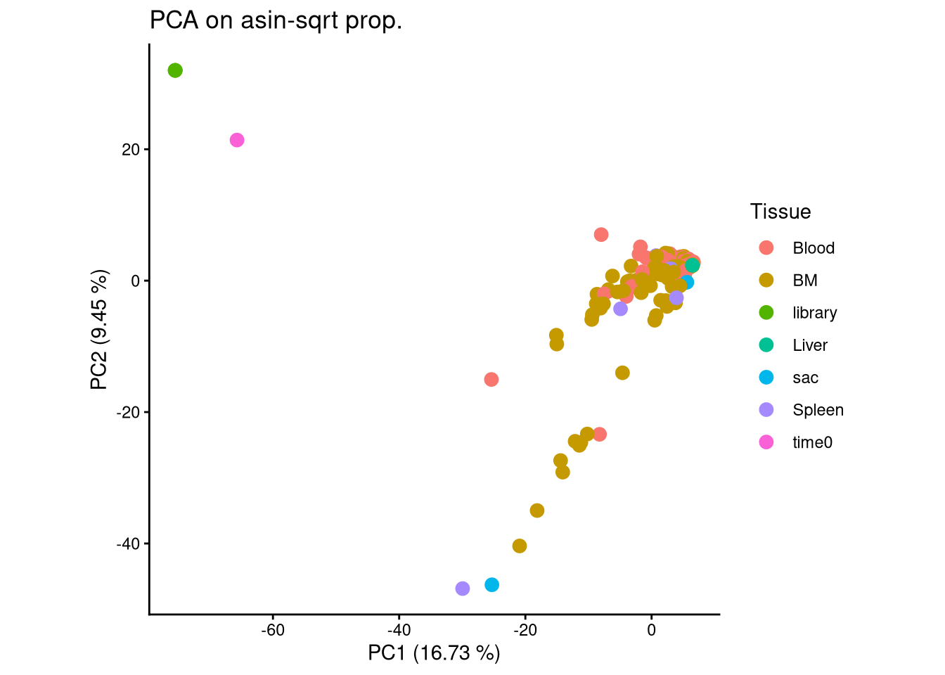

Delete “library” and “time0” samples in subsequent analysis.

xenoHSPC_recipient <- xenoHSPC_top[,!xenoHSPC_top$sampleMetadata$Tissue %in% c("library", "time0")]

dim(xenoHSPC_recipient)

[1] 918 195

xenoHSPC_recipient$sampleMetadata$Time <- factor(
  xenoHSPC_recipient$sampleMetadata$Time, 
  levels =  c("wk4", "wk6", "wk7", "wk9", "wk10", "wk11", "wk12", "wk14", "wk16", "wk18", "wk19", "wk20", "wk22", "wk24", "wk25", "wk27", "wk30", "wk33", "wk36", "wk37", "wk42", "wk43", "wk47", "sac") 
  )     

wk <- gsub("wk(\\d+)", "\\1", xenoHSPC_recipient$sampleMetadata$Time)
wk <- gsub("sac", 50, wk) ## assign "sac" pseudotime by wk50
wk <- as.numeric(wk)

xenoHSPC_recipient$sampleMetadata$Week <- wk

pca_results <- (assays(xenoHSPC_recipient)$proportion) %>% sqrt() %>% asin() %>% 
  t() %>% 
  prcomp()

var_pct <- pca_results$sdev^2 / sum(pca_results$sdev^2) * 100
var_pct

  [1] 1.479344e+01 8.330950e+00 6.287068e+00 6.226407e+00 5.363892e+00
  [6] 3.627028e+00 3.516160e+00 2.999774e+00 2.576212e+00 2.472176e+00
 [11] 2.120177e+00 2.056426e+00 1.752749e+00 1.626683e+00 1.583405e+00
 [16] 1.389448e+00 1.309808e+00 1.239237e+00 1.195308e+00 1.138141e+00
 [21] 1.078400e+00 1.013503e+00 9.053166e-01 8.702622e-01 8.214881e-01
 [26] 7.857411e-01 7.380047e-01 7.305955e-01 6.878795e-01 6.546646e-01
 [31] 6.074811e-01 5.935607e-01 5.740091e-01 5.513828e-01 5.301982e-01
 [36] 5.238409e-01 4.942603e-01 4.759932e-01 4.704834e-01 4.407335e-01
 [41] 4.333084e-01 4.196285e-01 4.009567e-01 3.861837e-01 3.748521e-01
 [46] 3.662801e-01 3.563715e-01 3.538795e-01 3.400533e-01 3.348882e-01
 [51] 3.207669e-01 3.113955e-01 3.031560e-01 3.011724e-01 2.953236e-01
 [56] 2.853936e-01 2.838217e-01 2.781898e-01 2.663242e-01 2.634376e-01
 [61] 2.406982e-01 2.397068e-01 2.272339e-01 2.198978e-01 2.192189e-01
 [66] 2.116993e-01 2.096951e-01 2.072526e-01 2.004909e-01 1.962941e-01
 [71] 1.911299e-01 1.861753e-01 1.810991e-01 1.723564e-01 1.701480e-01
 [76] 1.666642e-01 1.633386e-01 1.603920e-01 1.554791e-01 1.498141e-01
 [81] 1.453292e-01 1.406303e-01 1.380385e-01 1.348607e-01 1.313640e-01
 [86] 1.274998e-01 1.235760e-01 1.152278e-01 1.125916e-01 1.107482e-01
 [91] 1.079313e-01 1.058588e-01 1.016958e-01 9.807702e-02 9.558881e-02
 [96] 9.468148e-02 8.727559e-02 8.512717e-02 8.173793e-02 7.951066e-02
[101] 7.637967e-02 7.594063e-02 7.395949e-02 7.156617e-02 6.879921e-02
[106] 6.733569e-02 6.555393e-02 6.371865e-02 6.258242e-02 5.944996e-02
[111] 5.807566e-02 5.637390e-02 5.401405e-02 5.351594e-02 5.093370e-02
[116] 5.018407e-02 4.909521e-02 4.776852e-02 4.548049e-02 4.482061e-02
[121] 4.214630e-02 3.968405e-02 3.874588e-02 3.808117e-02 3.697447e-02
[126] 3.514576e-02 3.307821e-02 3.077555e-02 3.044347e-02 2.948776e-02
[131] 2.797135e-02 2.769691e-02 2.727003e-02 2.514839e-02 2.397377e-02
[136] 2.310491e-02 2.167158e-02 2.044579e-02 2.010012e-02 1.930558e-02
[141] 1.880420e-02 1.765411e-02 1.740390e-02 1.628787e-02 1.555388e-02
[146] 1.429623e-02 1.393612e-02 1.358735e-02 1.292522e-02 1.247998e-02
[151] 1.205023e-02 1.130288e-02 1.075463e-02 9.735549e-03 9.145263e-03
[156] 8.264110e-03 7.646805e-03 7.306899e-03 7.083384e-03 6.556232e-03
[161] 5.688634e-03 5.128788e-03 4.964275e-03 4.483613e-03 4.406028e-03
[166] 4.068626e-03 3.848206e-03 3.759551e-03 3.543005e-03 3.363469e-03
[171] 3.178208e-03 2.908354e-03 2.644241e-03 2.264792e-03 1.681031e-03
[176] 4.620949e-04 2.020341e-04 2.687296e-05 2.680569e-12 2.917491e-30
[181] 4.353056e-31 8.729848e-32 8.729848e-32 8.729848e-32 8.729848e-32
[186] 8.729848e-32 8.729848e-32 8.729848e-32 8.729848e-32 8.729848e-32
[191] 8.729848e-32 8.729848e-32 8.729848e-32 8.729848e-32 5.365644e-32

pca_df <- data.frame(
  PC1 = pca_results$x[, 1],
  PC2 = pca_results$x[, 2],
  xenoHSPC_recipient$sampleMetadata
)

ggplot PCA

ggplot(pca_df, aes(x = PC1, y = PC2, color = Donor)) +
  geom_point(size = 3) +
  labs(title = "PCA on asin-sqrt prop.", 
       x = paste0("PC1 (", round(var_pct[1], 2), " %)"), 
       y = paste0("PC2 (", round(var_pct[2], 2), " %)")) +
  theme_classic() +
  theme(aspect.ratio = 1)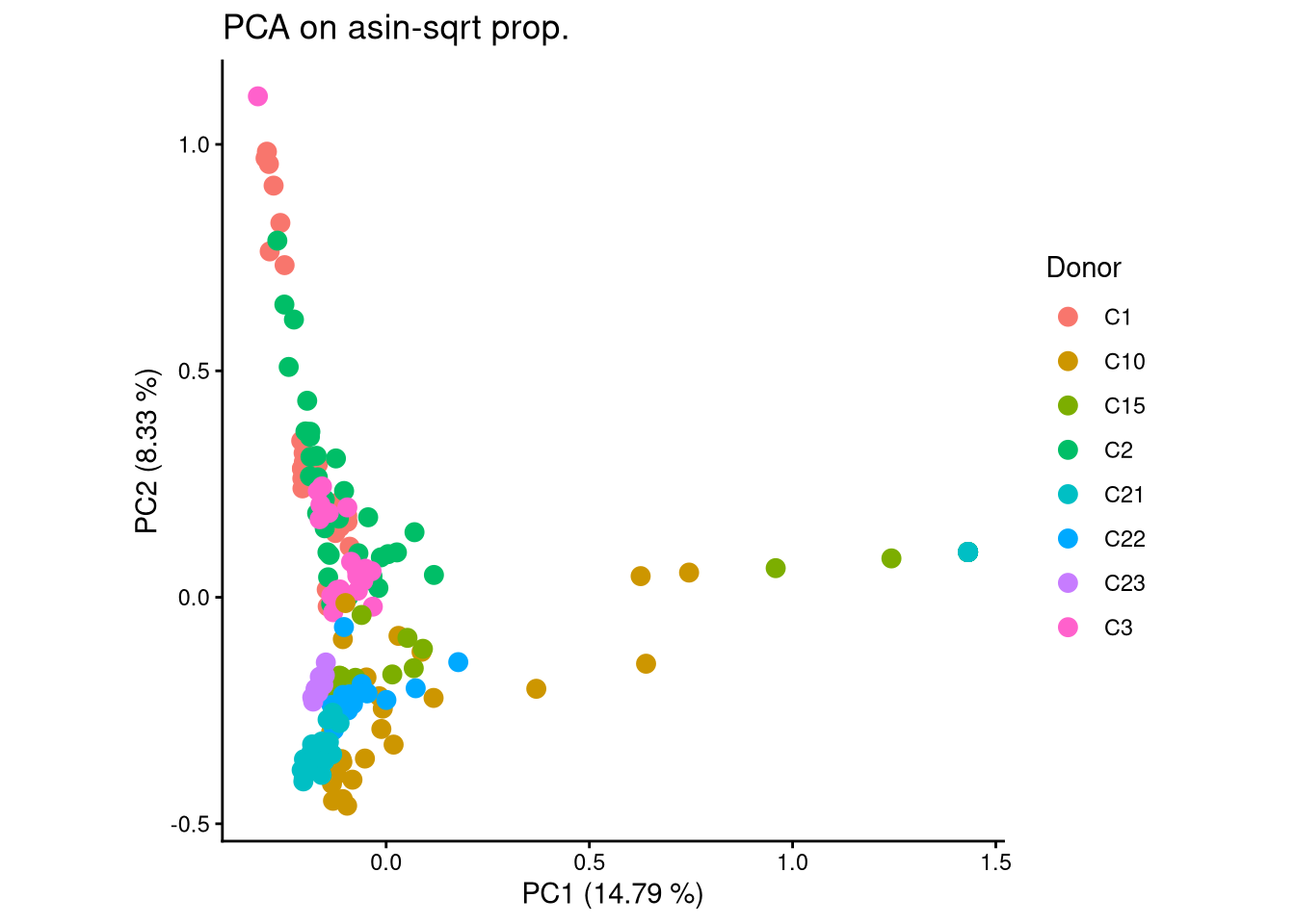

ggplot(pca_df, aes(x = PC1, y = PC2, color = Week)) +
  geom_point(size = 3) +
  labs(title = "PCA on asin-sqrt prop.", 
       x = paste0("PC1 (", round(var_pct[1], 2), " %)"), 
       y = paste0("PC2 (", round(var_pct[2], 2), " %)")) +
  theme_classic() +
  theme(aspect.ratio = 1)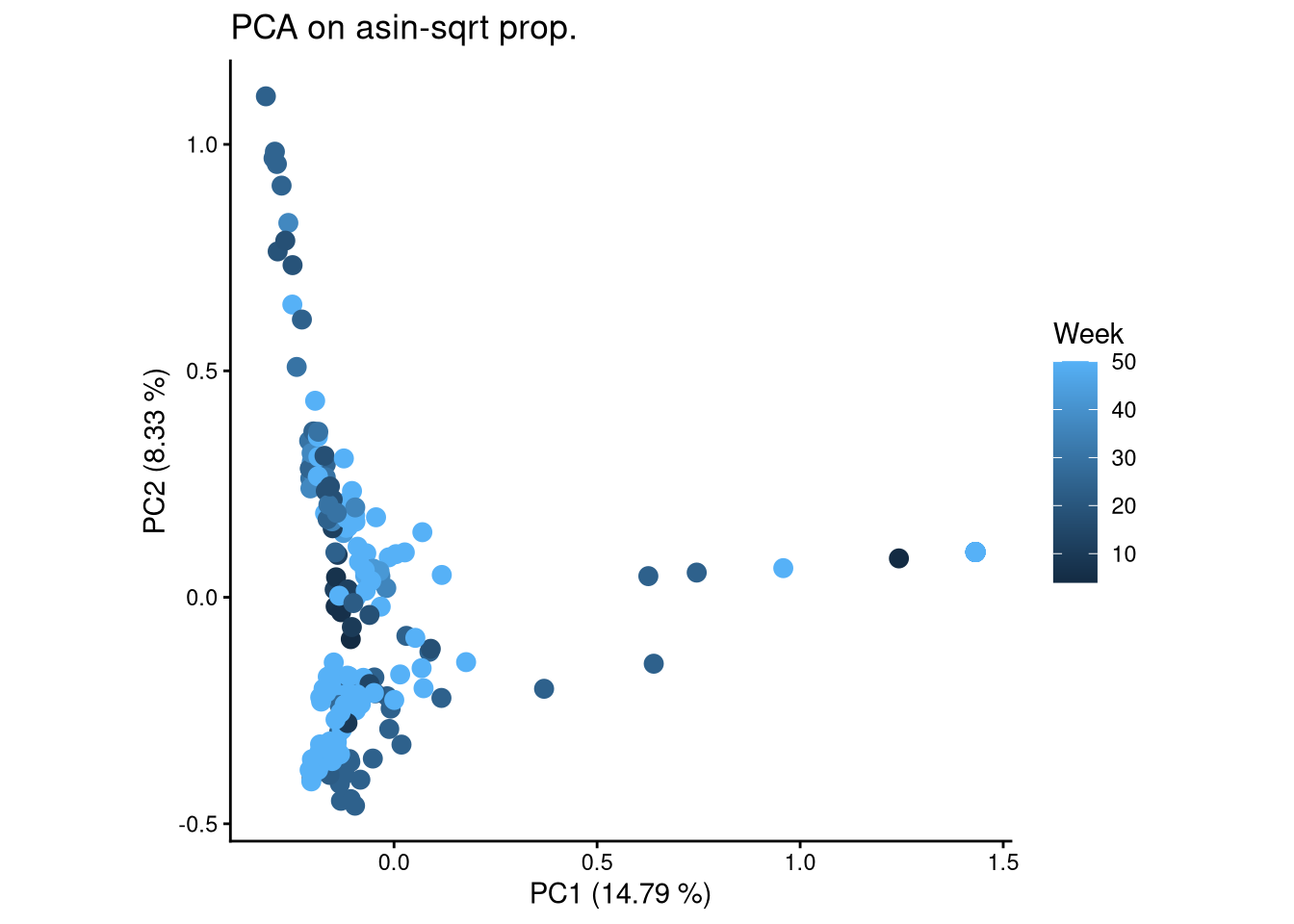

ggplot(pca_df, aes(x = PC1, y = PC2, color = Tissue)) +
  geom_point(size = 3) +
  labs(title = "PCA on asin-sqrt prop.", 
       x = paste0("PC1 (", round(var_pct[1], 2), " %)"), 
       y = paste0("PC2 (", round(var_pct[2], 2), " %)")) +
  theme_classic() +
  theme(aspect.ratio = 1)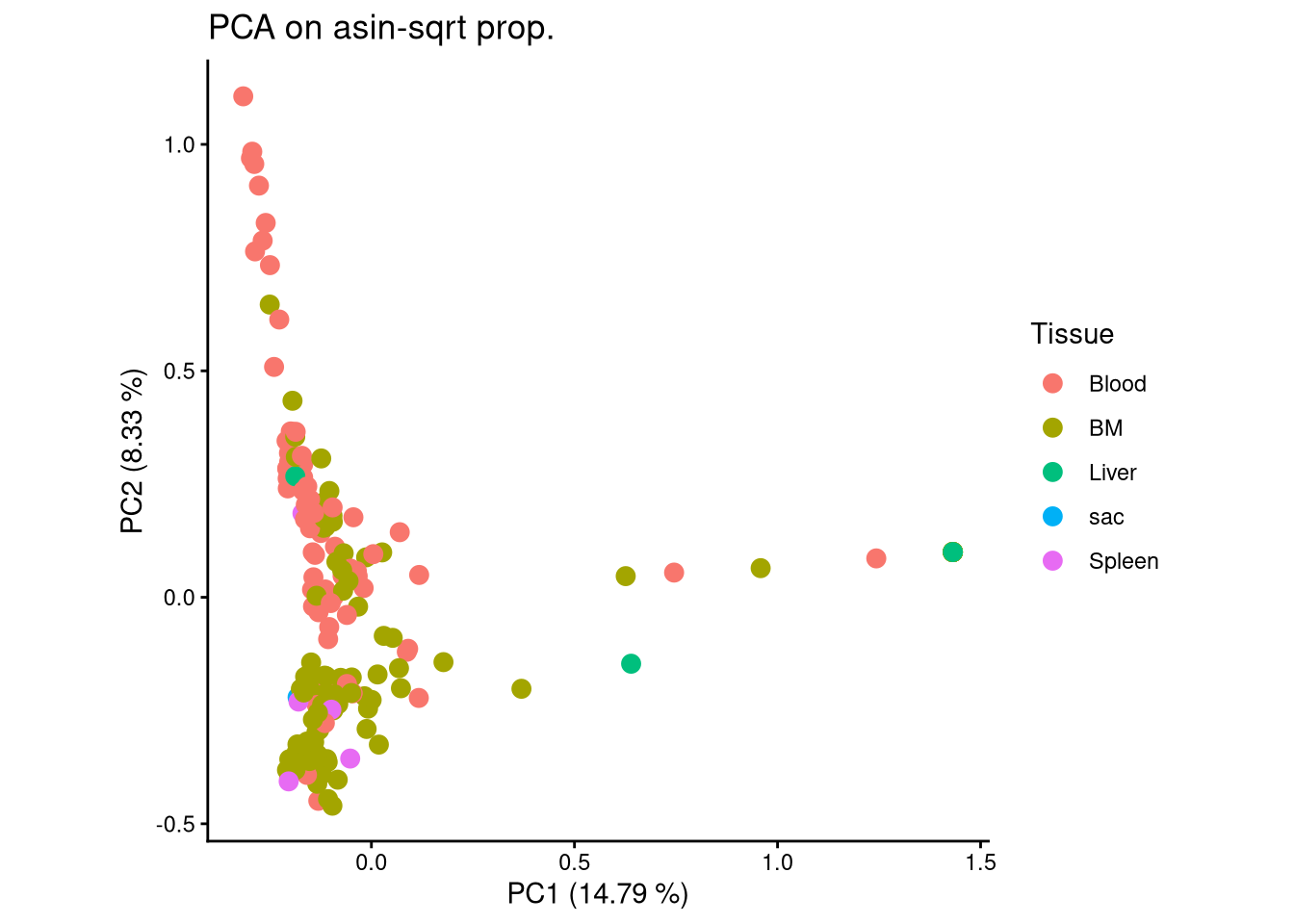

ggplot(pca_df, aes(x = PC1, y = PC2, color = Week)) +
  geom_point(size = 3) +
  labs(title = "PCA on asin-sqrt prop.", 
       x = paste0("PC1 (", round(var_pct[1], 2), " %)"), 
       y = paste0("PC2 (", round(var_pct[2], 2), " %)")) +
  theme_linedraw() +
  facet_grid(Donor~Celltype)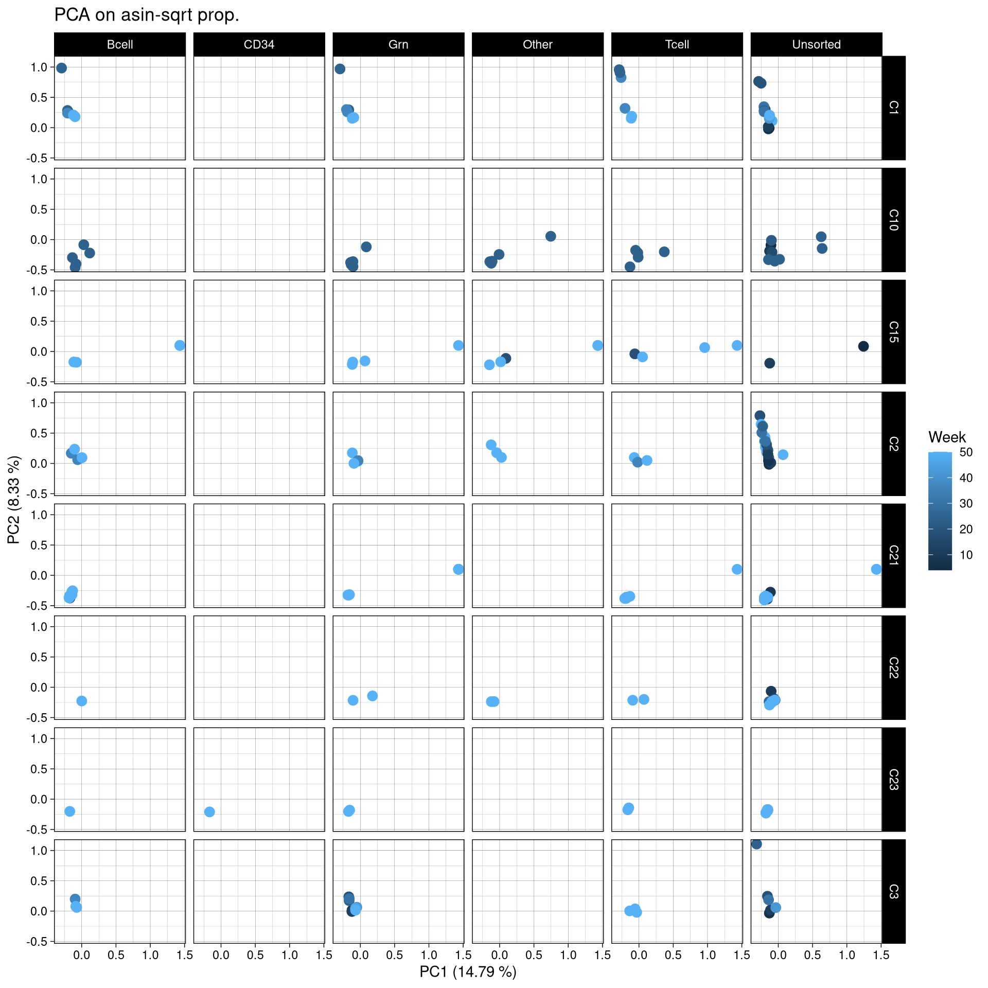

5.2 Plot propportion

## order samples
order_sample <- xenoHSPC_recipient$sampleMetadata %>% with(order(Donor, Tissue, Celltype, Time))

## assign unique names to samples
ps.counts <- assay(xenoHSPC_recipient)
colnames(ps.counts) <- make.unique(xenoHSPC_recipient$sampleMetadata$Donor)

## create bartools object
Donor_dge <- DGEList(
  counts = ps.counts, 
  group = xenoHSPC_recipient$sampleMetadata$Donor)

## plot 
plotBarcodeHistogram(Donor_dge, orderSamples = colnames(ps.counts)[order_sample])

Warning: Use of .data in tidyselect expressions was deprecated in tidyselect 1.2.0.
ℹ Please use `"barcode"` instead of `.data$barcode`
This warning is displayed once every 8 hours.
Call `lifecycle::last_lifecycle_warnings()` to see where this warning was
generated.

Warning: Use of .data in tidyselect expressions was deprecated in tidyselect 1.2.0.
ℹ Please use `"value"` instead of `.data$value`
This warning is displayed once every 8 hours.
Call `lifecycle::last_lifecycle_warnings()` to see where this warning was
generated.

Warning: Use of .data in tidyselect expressions was deprecated in tidyselect 1.2.0.
ℹ Please use `"name"` instead of `.data$name`
This warning is displayed once every 8 hours.
Call `lifecycle::last_lifecycle_warnings()` to see where this warning was
generated.

Warning: Use of .data in tidyselect expressions was deprecated in tidyselect 1.2.0.
ℹ Please use `"freq"` instead of `.data$freq`
This warning is displayed once every 8 hours.
Call `lifecycle::last_lifecycle_warnings()` to see where this warning was
generated.

Warning: The `guide` argument in `scale_*()` cannot be `FALSE`. This was deprecated in
ggplot2 3.3.4.
ℹ Please use "none" instead.
This warning is displayed once every 8 hours.
Call `lifecycle::last_lifecycle_warnings()` to see where this warning was
generated.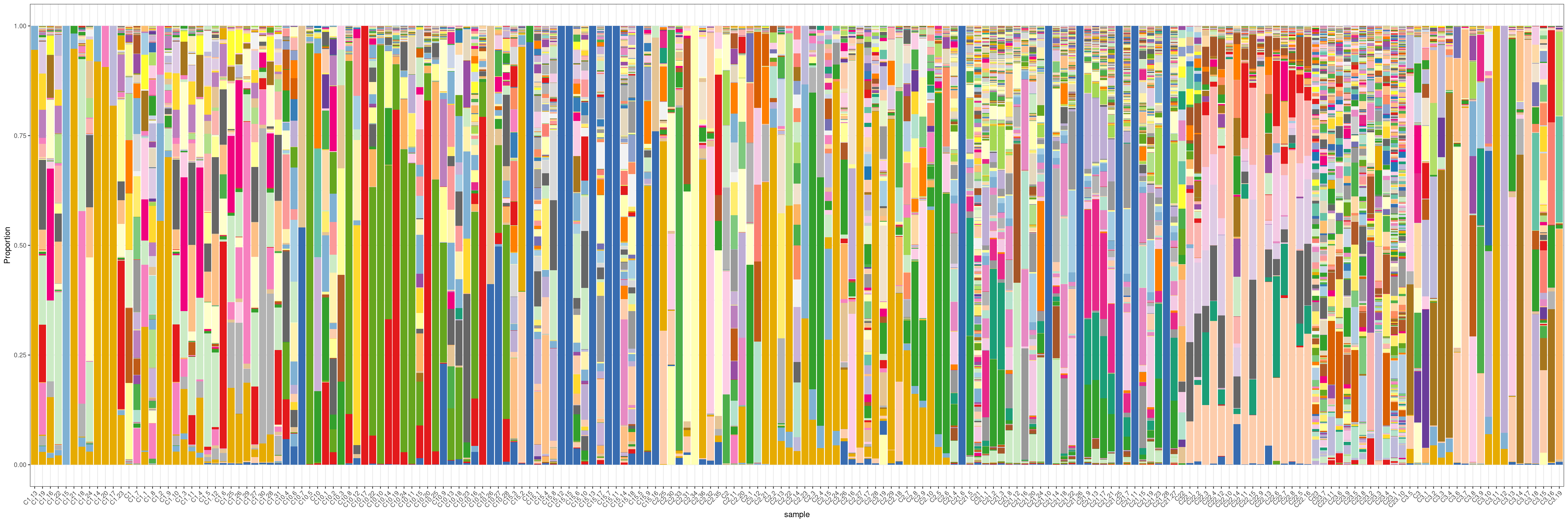

5.3 Heatmap

barbieQ::plotBarcodeHeatmap(
  xenoHSPC_recipient, sampleMetadata = xenoHSPC_recipient$sampleMetadata[,c(2,5,6,7,8)], splitSamples = T, sampleGroup = "Donor")

setting Donor as the primary factor in `sampleMetadata`.

The automatically generated colors map from the 1^st and 99^th of the
values in the matrix. There are outliers in the matrix whose patterns
might be hidden by this color mapping. You can manually set the color
to `col` argument.

Use `suppressMessages()` to turn off this message.

Following `at` are removed: NA, because no color was defined for them.
Following `at` are removed: NA, because no color was defined for them.
Following `at` are removed: NA, because no color was defined for them.

The automatically generated colors map from the 1^st and 99^th of the
values in the matrix. There are outliers in the matrix whose patterns
might be hidden by this color mapping. You can manually set the color
to `col` argument.

Use `suppressMessages()` to turn off this message.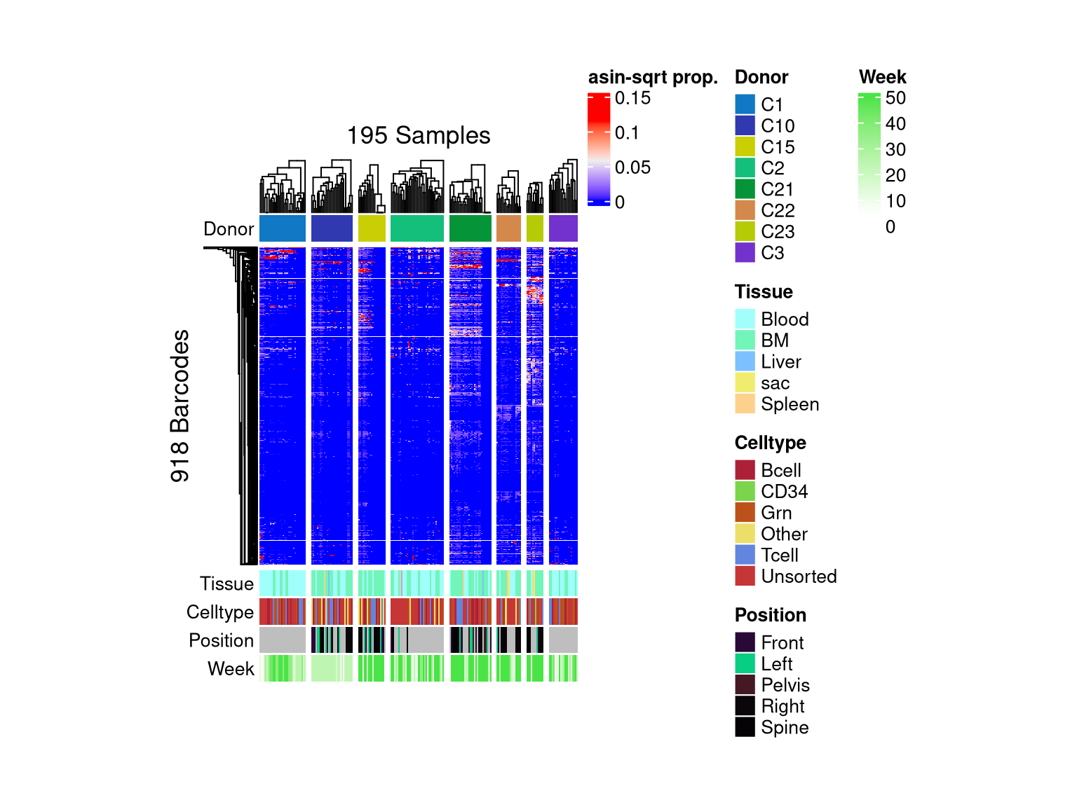

matrix color is mapped to `asin-sqrt proportion` but labeled by raw proportion.

Following `at` are removed: NA, because no color was defined for them.
Following `at` are removed: NA, because no color was defined for them.
Following `at` are removed: NA, because no color was defined for them.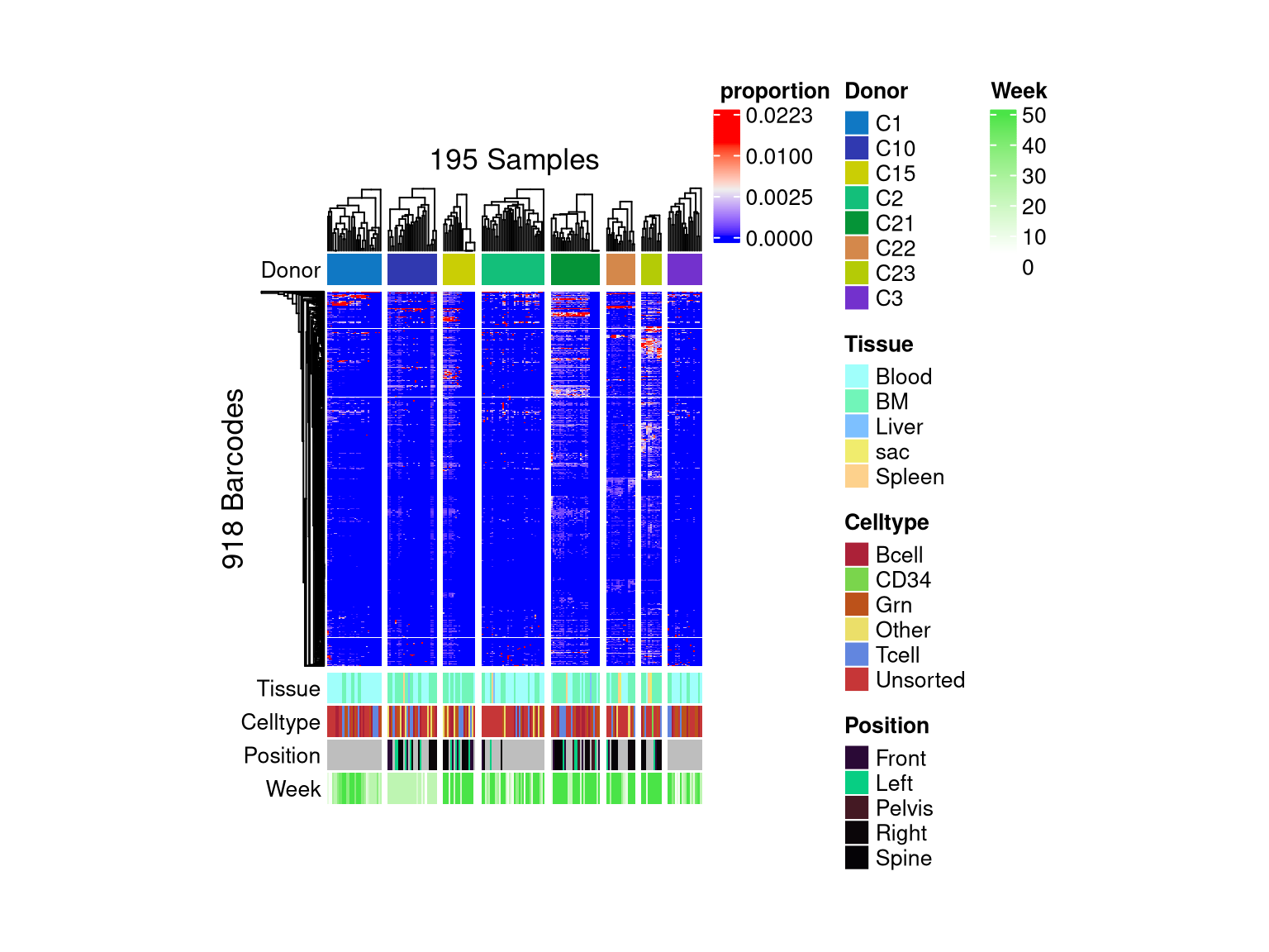

6 Subset samples of indivisual donors

QC samples

6.1 Donor C21

## subet C21 Donor samples
C21 <- xenoHSPC_recipient[, xenoHSPC_recipient$sampleMetadata$Donor == "C21"]

## flag C21 samples of extremely low libsize
colSums(assay(C21)) %>% sort()

       BMPelvis_T             Liver   BMFront_G...169        BMPelvis_G 
                2                 2                 4                 4 
  BMLeft_unsorted            wk22_G        BMPelvis_B   BMRight_B...175 
                5                10              3081              3183 
   BMLeft_G...173 BMPelvis_unsorted      Spleen...186   BMFront_T...168 
             4605              6645              6866              8667 
           wk22_B        wk14...160     wk22_unsorted  BMSpine_unsorted 
             9253             10201             10237             15348 
           wk22_T   BMSpine_G...181    BMLeft_B...171   BMRight_G...177 
            15382             18122             19473             21358 
              wk9   BMSpine_B...179   BMFront_B...167        wk20...161 
            21773             22775             32820             38310 
        BMRight_T   BMSpine_T...180  BMRight_unsorted  BMFront_unsorted 
            42697             51396             62162             62409 
   BMLeft_T...172 
            79018

flag_low_C21 <- colSums(assay(C21)) < 100
## remove the low libsize samples
C21 <- C21[, !flag_low_C21]
colSums(assay(C21)) %>% sort()

       BMPelvis_B   BMRight_B...175    BMLeft_G...173 BMPelvis_unsorted 
             3081              3183              4605              6645 
     Spleen...186   BMFront_T...168            wk22_B        wk14...160 
             6866              8667              9253             10201 
    wk22_unsorted  BMSpine_unsorted            wk22_T   BMSpine_G...181 
            10237             15348             15382             18122 
   BMLeft_B...171   BMRight_G...177               wk9   BMSpine_B...179 
            19473             21358             21773             22775 
  BMFront_B...167        wk20...161         BMRight_T   BMSpine_T...180 
            32820             38310             42697             51396 
 BMRight_unsorted  BMFront_unsorted    BMLeft_T...172 
            62162             62409             79018

## tag top barcodes within C21
C21$sampleMetadata %>% with(paste(Donor, Tissue, Celltype, Time)) %>% table()

.
   C21 Blood Bcell wk22    C21 Blood Tcell wk22 C21 Blood Unsorted wk14 
                      1                       1                       1 
C21 Blood Unsorted wk20 C21 Blood Unsorted wk22  C21 Blood Unsorted wk9 
                      1                       1                       1 
       C21 BM Bcell sac          C21 BM Grn sac        C21 BM Tcell sac 
                      5                       3                       4 
    C21 BM Unsorted sac C21 Spleen Unsorted sac 
                      4                       1

C21 <- tagTopBarcodes(C21, nSampleThreshold = 1)
plotBarcodePareto(C21)

Warning: Removed 10 rows containing missing values or values outside the scale range
(`geom_bar()`).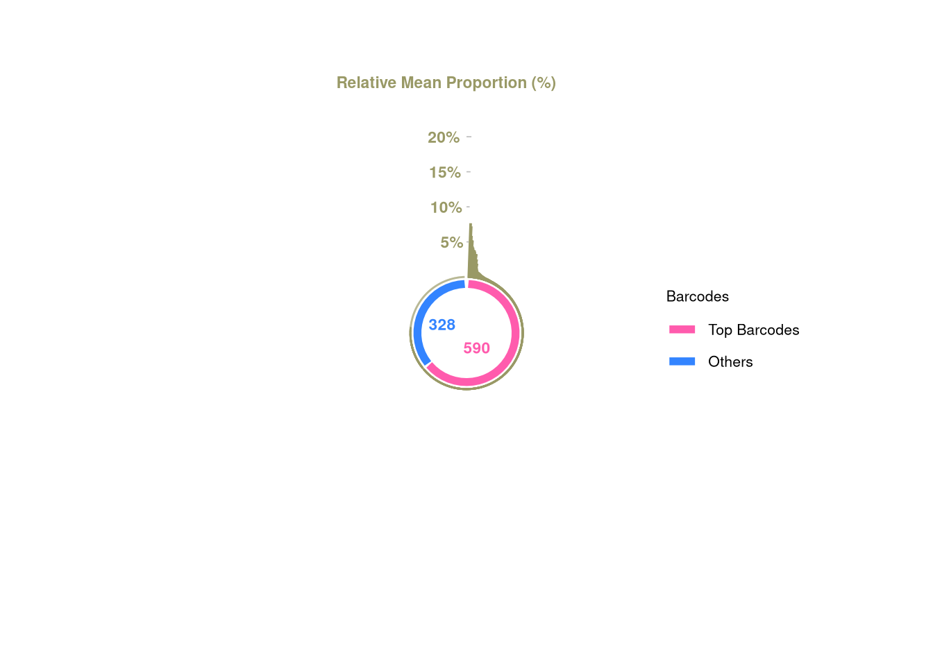

plotBarcodeSankey(C21)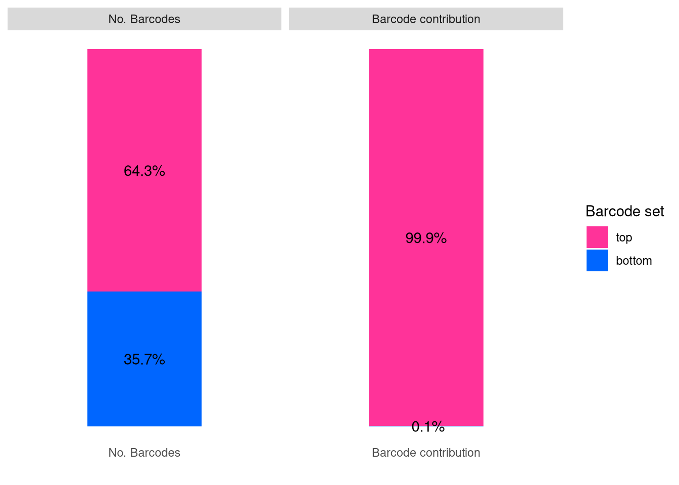

## filter top barcodes
C21 <- C21[C21@elementMetadata$isTopBarcode$isTop,]

barbieQ::plotBarcodeHeatmap(C21, sampleMetadata = C21$sampleMetadata[,c(5,6,7,8)])

setting Tissue as the primary factor in `sampleMetadata`.

The automatically generated colors map from the 1^st and 99^th of the
values in the matrix. There are outliers in the matrix whose patterns
might be hidden by this color mapping. You can manually set the color
to `col` argument.

Use `suppressMessages()` to turn off this message.

Following `at` are removed: NA, because no color was defined for them.
Following `at` are removed: NA, because no color was defined for them.
Following `at` are removed: NA, because no color was defined for them.

The automatically generated colors map from the 1^st and 99^th of the
values in the matrix. There are outliers in the matrix whose patterns
might be hidden by this color mapping. You can manually set the color
to `col` argument.

Use `suppressMessages()` to turn off this message.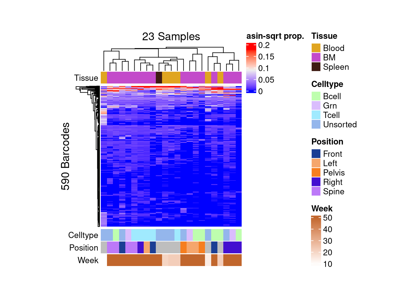

matrix color is mapped to `asin-sqrt proportion` but labeled by raw proportion.

Following `at` are removed: NA, because no color was defined for them.
Following `at` are removed: NA, because no color was defined for them.
Following `at` are removed: NA, because no color was defined for them.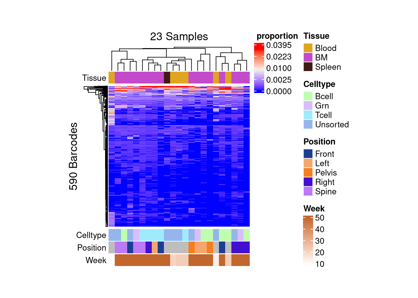

pca_results <- (assays(C21)$proportion) %>% sqrt() %>% asin() %>% 
  t() %>% 
  prcomp()

var_pct <- pca_results$sdev^2 / sum(pca_results$sdev^2) * 100
var_pct

 [1] 2.838868e+01 1.945461e+01 1.604830e+01 9.087066e+00 7.553164e+00
 [6] 4.218560e+00 3.457480e+00 2.044943e+00 1.719414e+00 1.537810e+00
[11] 1.094493e+00 9.574606e-01 8.023795e-01 7.000405e-01 6.082241e-01
[16] 5.635789e-01 4.785449e-01 4.352631e-01 3.336410e-01 2.606871e-01
[21] 1.578211e-01 9.782896e-02 5.165806e-31

pca_df <- data.frame(
  PC1 = pca_results$x[, 1],
  PC2 = pca_results$x[, 2],
  C21$sampleMetadata
)

ggplot(pca_df, aes(x = PC1, y = PC2, color = Week)) +
  geom_point(size = 3) +
  labs(title = "PCA on asin-sqrt prop.", 
       x = paste0("PC1 (", round(var_pct[1], 2), " %)"), 
       y = paste0("PC2 (", round(var_pct[2], 2), " %)")) +
  theme_classic() +
  theme(aspect.ratio = 1)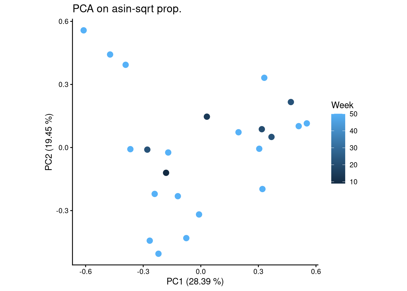

ggplot(pca_df, aes(x = PC1, y = PC2, color = Tissue)) +
  geom_point(size = 3) +
  labs(title = "PCA on asin-sqrt prop.", 
       x = paste0("PC1 (", round(var_pct[1], 2), " %)"), 
       y = paste0("PC2 (", round(var_pct[2], 2), " %)")) +
  theme_classic() +
  theme(aspect.ratio = 1)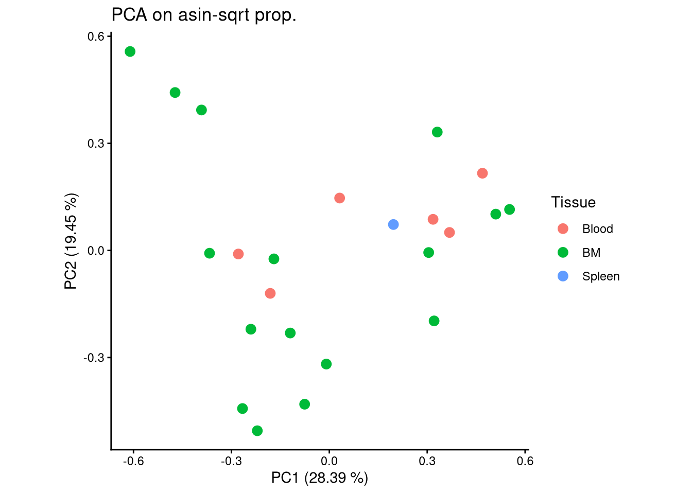

ggplot(pca_df, aes(x = PC1, y = PC2, color = Celltype)) +
  geom_point(size = 3) +
  labs(title = "PCA on asin-sqrt prop.", 
       x = paste0("PC1 (", round(var_pct[1], 2), " %)"), 
       y = paste0("PC2 (", round(var_pct[2], 2), " %)")) +
  theme_classic() +
  theme(aspect.ratio = 1)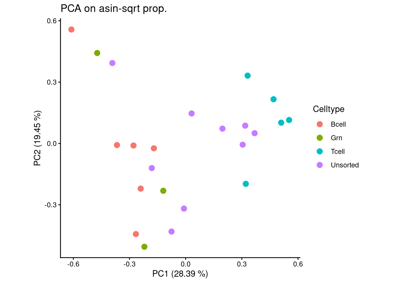

6.2 Donor C22

## subet C21 Donor samples
C22 <- xenoHSPC_recipient[, xenoHSPC_recipient$sampleMetadata$Donor == "C22"]

## flag C22 samples of extremely low libsize
colSums(assay(C22)) %>% sort()

             wk14...143                    wk10                    wk27 
                   4715                    7160                   14534 
       BM_Right_T...151 BM_Right_unsorted...150                     sac 
                  16079                   16980                   23283 
                   wk33                BM_Front              wk20...144 
                  26871                   29741                   41579 
       BM_Right_G...152                 BM_Left              BM_Spine_O 
                  44421                   67066                   93833 
           Spleen...158              BM_Right_O        BM_Spine_B...154 
                 104606                  116938                  124739 
       BM_Spine_T...155        BM_Spine_G...156 
                 140737                  258357

## tag top barcodes within C22
C22$sampleMetadata %>% with(paste(Donor, Tissue, Celltype, Time)) %>% table()

.
C22 Blood Unsorted wk10 C22 Blood Unsorted wk14 C22 Blood Unsorted wk20 
                      1                       1                       1 
C22 Blood Unsorted wk27 C22 Blood Unsorted wk33        C22 BM Bcell sac 
                      1                       1                       1 
         C22 BM Grn sac        C22 BM Other sac        C22 BM Tcell sac 
                      2                       2                       2 
    C22 BM Unsorted sac    C22 sac Unsorted sac C22 Spleen Unsorted sac 
                      3                       1                       1

C22 <- tagTopBarcodes(C22, nSampleThreshold = 1)
plotBarcodePareto(C22)

Warning: Removed 11 rows containing missing values or values outside the scale range
(`geom_bar()`).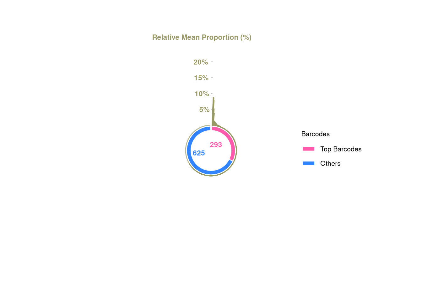

plotBarcodeSankey(C22)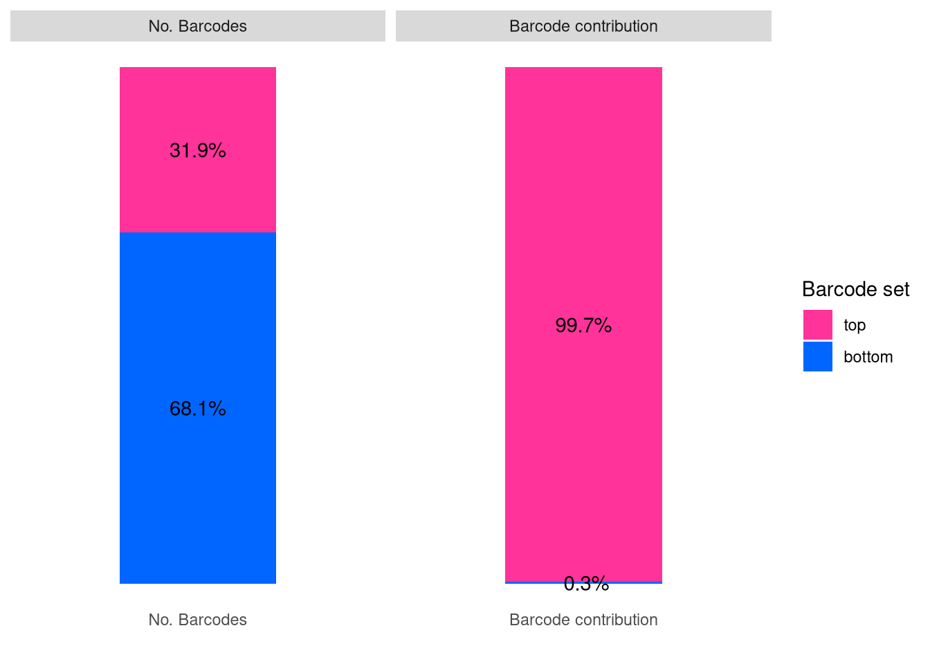

## filter top barcodes
C22 <- C22[C22@elementMetadata$isTopBarcode$isTop,]

barbieQ::plotBarcodeHeatmap(C22, sampleMetadata = C22$sampleMetadata[,c(5,6,7,8)])

setting Tissue as the primary factor in `sampleMetadata`.

The automatically generated colors map from the 1^st and 99^th of the
values in the matrix. There are outliers in the matrix whose patterns
might be hidden by this color mapping. You can manually set the color
to `col` argument.

Use `suppressMessages()` to turn off this message.

Following `at` are removed: NA, because no color was defined for them.
Following `at` are removed: NA, because no color was defined for them.
Following `at` are removed: NA, because no color was defined for them.

The automatically generated colors map from the 1^st and 99^th of the
values in the matrix. There are outliers in the matrix whose patterns
might be hidden by this color mapping. You can manually set the color
to `col` argument.

Use `suppressMessages()` to turn off this message.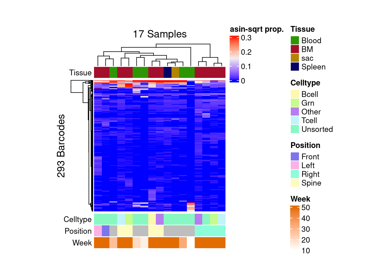

matrix color is mapped to `asin-sqrt proportion` but labeled by raw proportion.

Following `at` are removed: NA, because no color was defined for them.
Following `at` are removed: NA, because no color was defined for them.
Following `at` are removed: NA, because no color was defined for them.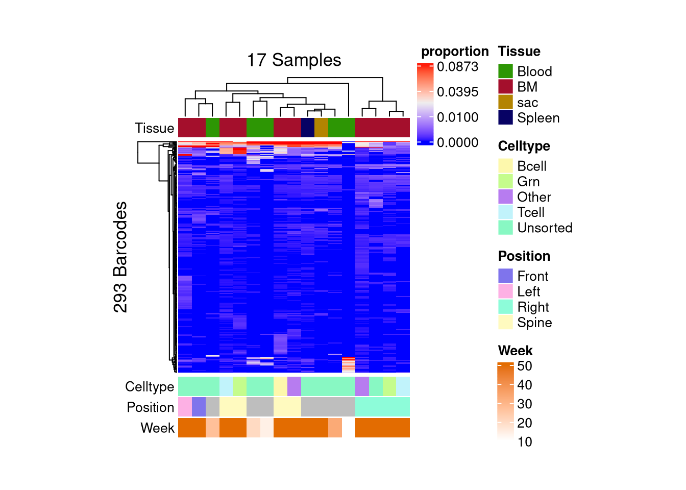

pca_results <- (assays(C22)$proportion) %>% sqrt() %>% asin() %>% 
  t() %>% 
  prcomp()

var_pct <- pca_results$sdev^2 / sum(pca_results$sdev^2) * 100
var_pct

 [1] 4.095180e+01 2.252903e+01 1.360985e+01 8.760720e+00 3.715730e+00
 [6] 2.789228e+00 2.416066e+00 1.947791e+00 9.175729e-01 5.576470e-01
[11] 5.251057e-01 4.346193e-01 3.103011e-01 2.287105e-01 1.955388e-01
[16] 1.102881e-01 4.351721e-31

pca_df <- data.frame(
  PC1 = pca_results$x[, 1],
  PC2 = pca_results$x[, 2],
  C22$sampleMetadata
)

ggplot(pca_df, aes(x = PC1, y = PC2, color = Week)) +
  geom_point(size = 3) +
  labs(title = "PCA on asin-sqrt prop.", 
       x = paste0("PC1 (", round(var_pct[1], 2), " %)"), 
       y = paste0("PC2 (", round(var_pct[2], 2), " %)")) +
  theme_classic() +
  theme(aspect.ratio = 1)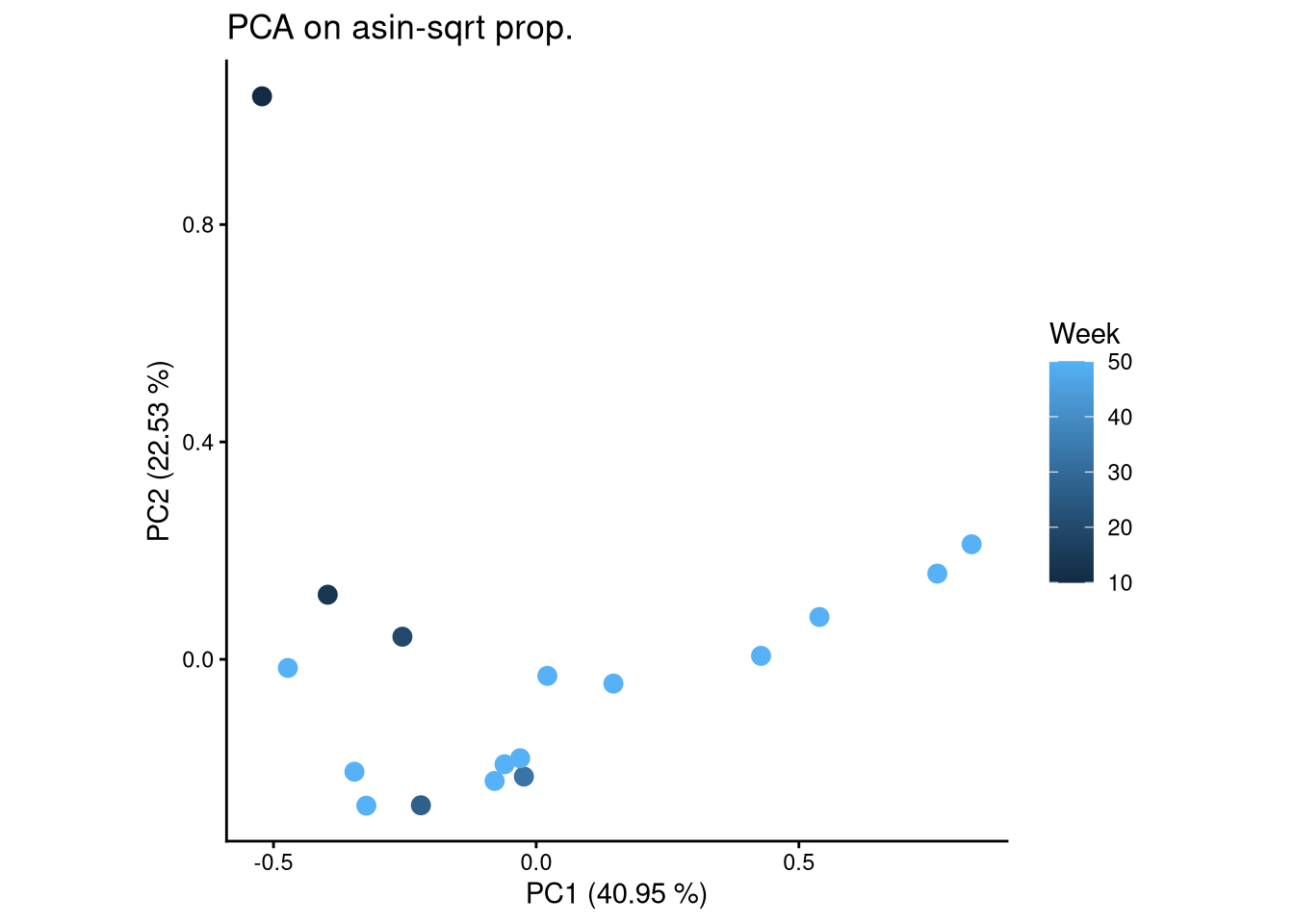

ggplot(pca_df, aes(x = PC1, y = PC2, color = Tissue)) +
  geom_point(size = 3) +
  labs(title = "PCA on asin-sqrt prop.", 
       x = paste0("PC1 (", round(var_pct[1], 2), " %)"), 
       y = paste0("PC2 (", round(var_pct[2], 2), " %)")) +
  theme_classic() +
  theme(aspect.ratio = 1)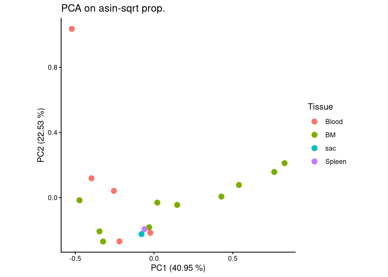

ggplot(pca_df, aes(x = PC1, y = PC2, color = Celltype)) +
  geom_point(size = 3) +
  labs(title = "PCA on asin-sqrt prop.", 
       x = paste0("PC1 (", round(var_pct[1], 2), " %)"), 
       y = paste0("PC2 (", round(var_pct[2], 2), " %)")) +
  theme_classic() +
  theme(aspect.ratio = 1)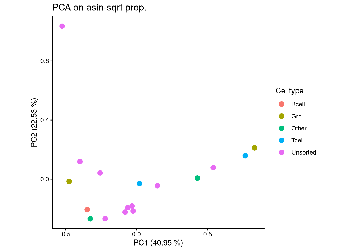

6.3 Donor C23

## subet C23 Donor samples
C23 <- xenoHSPC_recipient[, xenoHSPC_recipient$sampleMetadata$Donor == "C23"]

## flag C23 samples of extremely low libsize
colSums(assay(C23)) %>% sort()

                   wk11        BM_Right_G...194        BM_Spine_T...196 
                   7784                   93935                   94511 
       BM_Right_T...193        BM_Spine_B...195                     Sac 
                  98137                  142005                  151487 
       BM_Spine_G...197       BM_Front_unsorted                 BM_CD34 
                 159167                  175573                  196161 
BM_Right_unsorted...192        BM_Left_unsorted            Spleen...198 
                 231010                  249339                  288396

## tag top barcodes within C23
C23$sampleMetadata %>% with(paste(Donor, Tissue, Celltype, Time)) %>% table()

.
C23 Blood Unsorted wk11        C23 BM Bcell sac         C23 BM CD34 sac 
                      1                       1                       1 
         C23 BM Grn sac        C23 BM Tcell sac     C23 BM Unsorted sac 
                      2                       2                       3 
   C23 sac Unsorted sac C23 Spleen Unsorted sac 
                      1                       1

C23 <- tagTopBarcodes(C23, nSampleThreshold = 1)
plotBarcodePareto(C23)

Warning: Removed 10 rows containing missing values or values outside the scale range
(`geom_bar()`).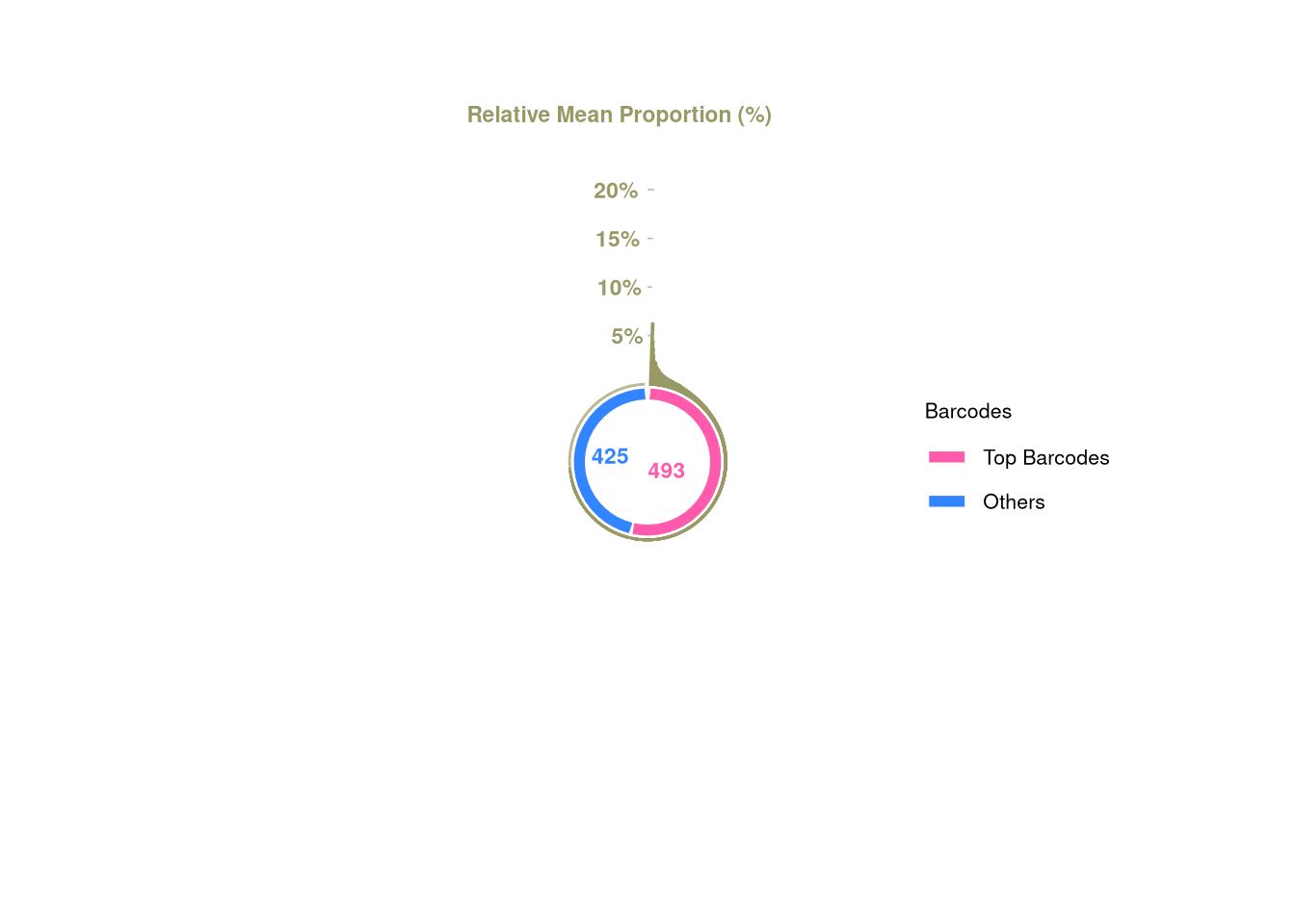

plotBarcodeSankey(C23)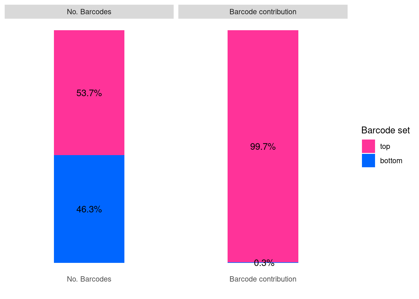

## filter top barcodes
C23 <- C23[C23@elementMetadata$isTopBarcode$isTop,]

barbieQ::plotBarcodeHeatmap(C23, sampleMetadata = C23$sampleMetadata[,c(5,6,7,8)])

setting Tissue as the primary factor in `sampleMetadata`.

The automatically generated colors map from the 1^st and 99^th of the
values in the matrix. There are outliers in the matrix whose patterns
might be hidden by this color mapping. You can manually set the color
to `col` argument.

Use `suppressMessages()` to turn off this message.

Following `at` are removed: NA, because no color was defined for them.
Following `at` are removed: NA, because no color was defined for them.
Following `at` are removed: NA, because no color was defined for them.

The automatically generated colors map from the 1^st and 99^th of the
values in the matrix. There are outliers in the matrix whose patterns
might be hidden by this color mapping. You can manually set the color
to `col` argument.

Use `suppressMessages()` to turn off this message.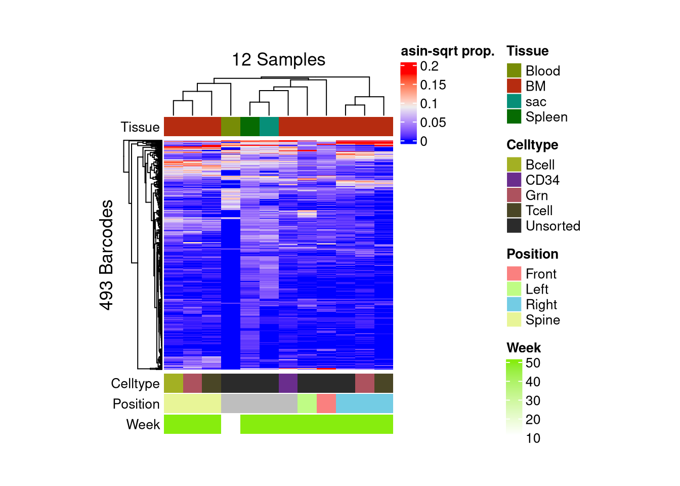

matrix color is mapped to `asin-sqrt proportion` but labeled by raw proportion.

Following `at` are removed: NA, because no color was defined for them.
Following `at` are removed: NA, because no color was defined for them.
Following `at` are removed: NA, because no color was defined for them.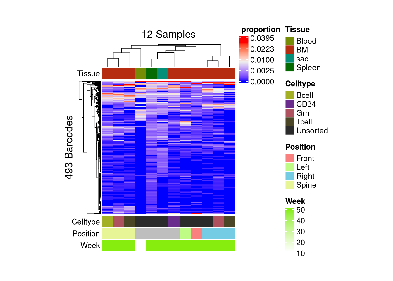

pca_results <- (assays(C23)$proportion) %>% sqrt() %>% asin() %>% 
  t() %>% 
  prcomp()

var_pct <- pca_results$sdev^2 / sum(pca_results$sdev^2) * 100
var_pct

 [1] 3.219522e+01 1.869976e+01 1.438379e+01 1.071146e+01 8.224041e+00
 [6] 6.535110e+00 3.321768e+00 1.942473e+00 1.630203e+00 1.493167e+00
[11] 8.630028e-01 1.097978e-30

pca_df <- data.frame(
  PC1 = pca_results$x[, 1],
  PC2 = pca_results$x[, 2],
  C23$sampleMetadata
)

ggplot(pca_df, aes(x = PC1, y = PC2, color = Week)) +
  geom_point(size = 3) +
  labs(title = "PCA on asin-sqrt prop.", 
       x = paste0("PC1 (", round(var_pct[1], 2), " %)"), 
       y = paste0("PC2 (", round(var_pct[2], 2), " %)")) +
  theme_classic() +
  theme(aspect.ratio = 1)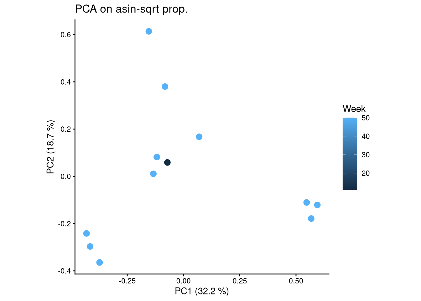

ggplot(pca_df, aes(x = PC1, y = PC2, color = Tissue)) +
  geom_point(size = 3) +
  labs(title = "PCA on asin-sqrt prop.", 
       x = paste0("PC1 (", round(var_pct[1], 2), " %)"), 
       y = paste0("PC2 (", round(var_pct[2], 2), " %)")) +
  theme_classic() +
  theme(aspect.ratio = 1)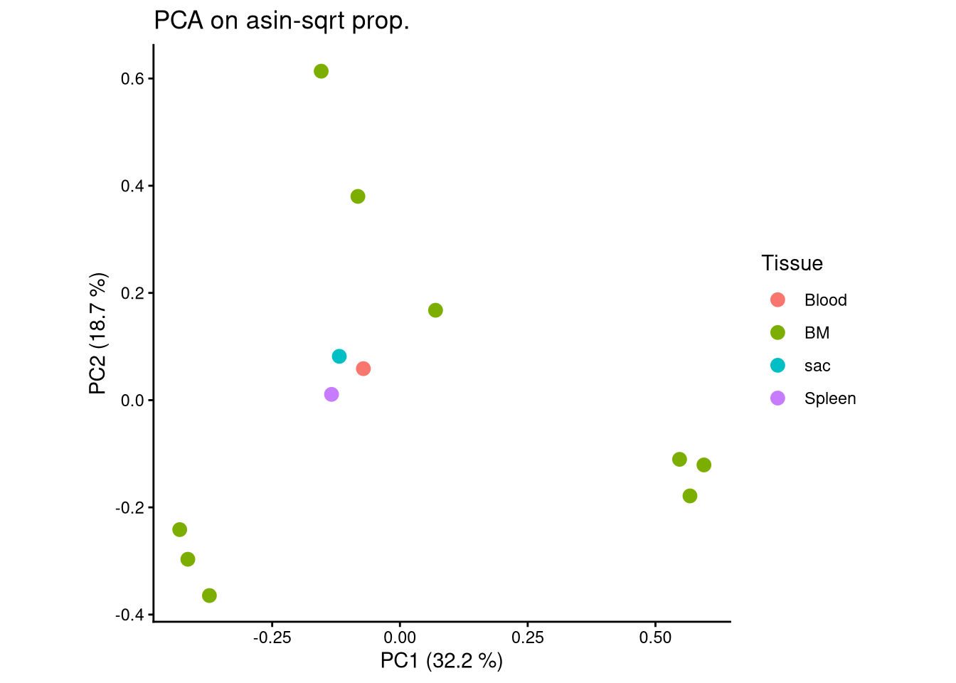

ggplot(pca_df, aes(x = PC1, y = PC2, color = Celltype)) +
  geom_point(size = 3) +
  labs(title = "PCA on asin-sqrt prop.", 
       x = paste0("PC1 (", round(var_pct[1], 2), " %)"), 
       y = paste0("PC2 (", round(var_pct[2], 2), " %)")) +
  theme_classic() +
  theme(aspect.ratio = 1)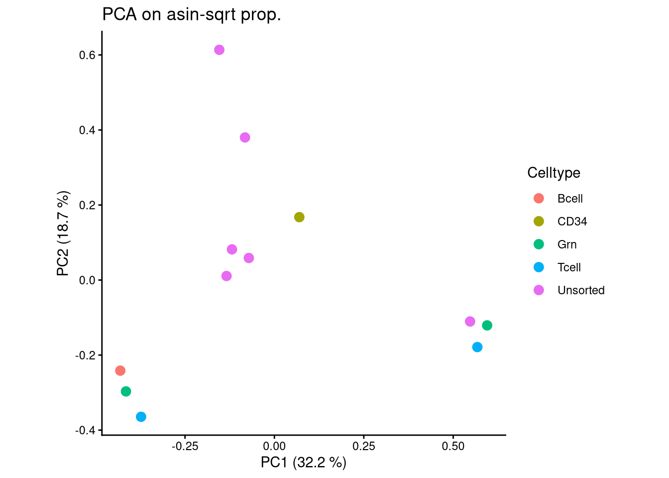

7 Plot proportion

7.1 Donor C21

## order samples
C21_id <- C21$sampleMetadata %>% with(paste(Tissue, Celltype, Position, Time, sep = "."))
order_C21 <- order(C21$sampleMetadata %>% with(paste(Tissue, Celltype, Position, Week, sep = ".")))

## create bartools object
C21_count <- assay(C21)
colnames(C21_count) <- C21_id

C21_dge <- DGEList(
  counts = C21_count, 
  group = C21$sampleMetadata$Donor)

## plot 
plotBarcodeHistogram(C21_dge, orderSamples = C21_id[order_C21]) + 
  labs(title = "HSPC xenograft: Donor C21") -> p_prop_C21

7.2 Donor C22

## order samples
C22_id <- C22$sampleMetadata %>% with(paste(Tissue, Position, Celltype, Time, sep = "."))
order_C22 <- order(C22$sampleMetadata %>% with(paste(Tissue, Position, Celltype, Week, sep = ".")))

## create bartools object
C22_count <- assay(C22)
colnames(C22_count) <- C22_id

C22_dge <- DGEList(
  counts = C22_count, 
  group = C22$sampleMetadata$Donor)

## plot 
plotBarcodeHistogram(C22_dge, orderSamples = C22_id[order_C22]) + 
  labs(title = "HSPC xenograft: Donor C22") -> p_prop_C22

7.3 Donor C23

## order samples
C23_id <- C23$sampleMetadata %>% with(paste(Tissue, Position, Celltype, Time, sep = "."))
order_C23 <- order(C23$sampleMetadata %>% with(paste(Tissue, Position, Celltype, Week, sep = ".")))

## create bartools object
C23_count <- assay(C23)
colnames(C23_count) <- C23_id

C23_dge <- DGEList(
  counts = C23_count, 
  group = C23$sampleMetadata$Donor)

## plot 
plotBarcodeHistogram(C23_dge, orderSamples = C23_id[order_C23]) + 
  labs(title = "HSPC xenograft: Donor C23") -> p_prop_C23

7.4 FS2A,C,E: prop. of three donors

p_prop_C21 / p_prop_C22 / p_prop_C23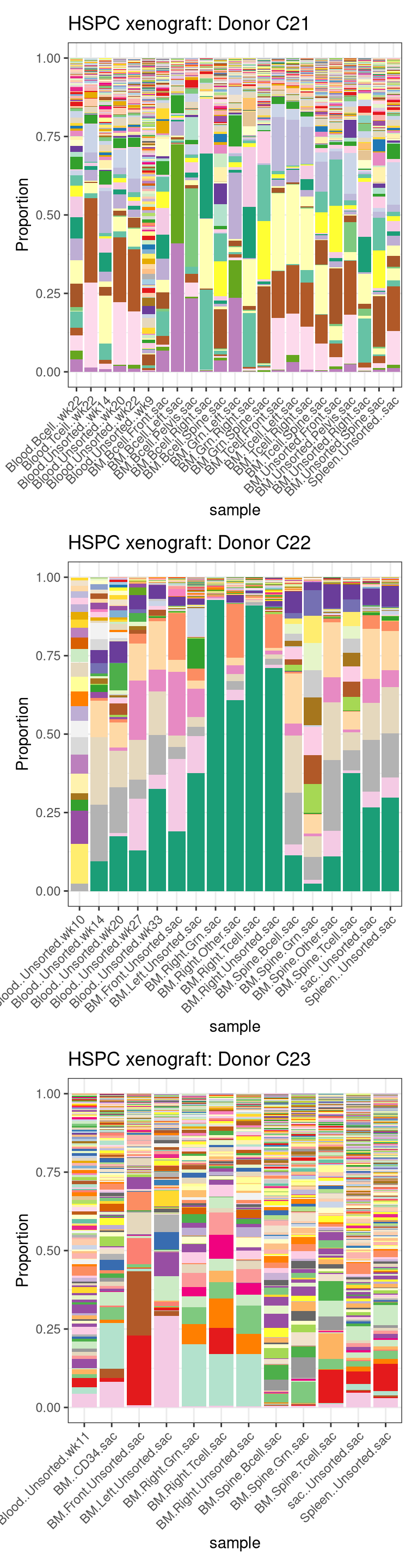

8 Type I error rate

8.1 Donor C21

Negative simulation

avoid running this chunk during rendering. global_all_loops was saved from the first run.

results_negsi <- suppressMessages({
  random_sampling(barbieQ = C21, loop_times = 100)
  })

## `random_sampling()` save the simulations to global environment as `global_all_loops`
save(global_all_loops, file = "output/xenoC21_negative_simulation.rda")

load results

## loading random sampling results to avoid running it repeatedly
load("output/xenoC21_negative_simulation.rda")

# extract results from the loops
end_sampling <- floor(ncol(C21)/2)

## extract FPR
all_FPR <- lapply(seq(3:end_sampling), function(n) {
  global_all_loops[[n]]$FPR
})
df_FPR_C21 <- do.call(rbind, all_FPR)

plot FPR

df_FPR_C21$N_Samples <- as.factor(df_FPR_C21$N_Samples)

## Diff_Prop
## reshape the data to fit methods for testing
df_FPR_C21_long <- df_FPR_C21 %>%
  pivot_longer(cols = starts_with("Prop_"),
               names_to = "Method",
               values_to = "Pval_Prop") %>%
  mutate(Method = factor(Method, levels = c("Prop_asin", "Prop_logit", "Prop_noTrans"),
                         labels = c("asin-sqrt", "logit", "no trans.")))

P_FPR_prop_C21 <- ggplot(
  df_FPR_C21_long, aes(x = factor(N_Samples), y = Pval_Prop, color = Method)) +
  geom_boxplot(outlier.shape = 1, position = position_dodge(width = 0.7)) +
  # geom_jitter(size = 1, position = position_dodge(width = 0.7)) +
  geom_hline(yintercept = 0.05, linetype = "dashed", color = "black") +
  # coord_cartesian(ylim = c(0, 0.2)) + 
  labs(
       y = "Fraction of P-Value < 0.05",
       x = "Number of samples per group",
       # title = "C21",
       subtitle = "Differential proportion test") +
  # facet_wrap(~Method, scales = "free_y") +
  theme_classic() +
  theme(legend.position = "top")

## Diff_Occ
P_FPR_occ_C21 <- ggplot(
  df_FPR_C21, aes(x = factor(N_Samples), y = Occ_firth)) +
  geom_boxplot(outlier.shape = 1, position = position_dodge(width = 0.7)) +
  # geom_jitter(size = 1, position = position_dodge(width = 0.7)) +
  geom_hline(yintercept = 0.05, linetype = "dashed", color = "black") +
  scale_color_manual(values = c("Differential occurrrence test" = "black")) +
  # coord_cartesian(ylim = c(0, 0.2)) + 
  labs(
       y = "Fraction of P-Value < 0.05",
       x = "Number of samples per group",
       titlte = "",
       subtitle = "Differential occurrence test") +
  theme_classic() +
  theme(legend.position = "top")

8.2 Donor C22

Negative simulation

avoid running this chunk during rendering. global_all_loops was saved from the first run.

results_negsi <- suppressMessages({
  random_sampling(barbieQ = C22, loop_times = 100)
  })

## `random_sampling()` save the simulations to global environment as `global_all_loops`
save(global_all_loops, file = "output/xenoC22_negative_simulation.rda")

load results

## loading random sampling results to avoid running it repeatedly
load("output/xenoC22_negative_simulation.rda")

# extract results from the loops
end_sampling <- floor(ncol(C22)/2)

## extract FPR
all_FPR <- lapply(seq(3:end_sampling), function(n) {
  global_all_loops[[n]]$FPR
})
df_FPR_C22 <- do.call(rbind, all_FPR)

plot FPR

df_FPR_C22$N_Samples <- as.factor(df_FPR_C22$N_Samples)

## Diff_Prop
## reshape the data to fit methods for testing
df_FPR_C22_long <- df_FPR_C22 %>%
  pivot_longer(cols = starts_with("Prop_"),
               names_to = "Method",
               values_to = "Pval_Prop") %>%
  mutate(Method = factor(Method, levels = c("Prop_asin", "Prop_logit", "Prop_noTrans"),
                         labels = c("asin-sqrt", "logit", "no trans.")))

P_FPR_prop_C22 <- ggplot(
  df_FPR_C22_long, aes(x = factor(N_Samples), y = Pval_Prop, color = Method)) +
  geom_boxplot(outlier.shape = 1, position = position_dodge(width = 0.7)) +
  # geom_jitter(size = 1, position = position_dodge(width = 0.7)) +
  geom_hline(yintercept = 0.05, linetype = "dashed", color = "black") +
  # coord_cartesian(ylim = c(0, 0.2)) + 
  labs(
       y = "Fraction of P-Value < 0.05",
       x = "Number of samples per group",
       # title = "C22",
       subtitle = "Differential proportion test") +
  # facet_wrap(~Method, scales = "free_y") +
  theme_classic() +
  theme(legend.position = "top")

## Diff_Occ
P_FPR_occ_C22 <- ggplot(
  df_FPR_C22, aes(x = factor(N_Samples), y = Occ_firth)) +
  geom_boxplot(outlier.shape = 1, position = position_dodge(width = 0.7)) +
  # geom_jitter(size = 1, position = position_dodge(width = 0.7)) +
  geom_hline(yintercept = 0.05, linetype = "dashed", color = "black") +
  scale_color_manual(values = c("Differential occurrrence test" = "black")) +
  # coord_cartesian(ylim = c(0, 0.2)) + 
  labs(
       y = "Fraction of P-Value < 0.05",
       x = "Number of samples per group",
       titlte = "",
       subtitle = "Differential occurrence test") +
  theme_classic() +
  theme(legend.position = "top")

8.3 Donor C23

Negative simulation

avoid running this chunk during rendering. global_all_loops was saved from the first run.

results_negsi <- suppressMessages({
  random_sampling(barbieQ = C23, loop_times = 100)
  })

## `random_sampling()` save the simulations to global environment as `global_all_loops`
save(global_all_loops, file = "output/xenoC23_negative_simulation.rda")

load results

## loading random sampling results to avoid running it repeatedly
load("output/xenoC23_negative_simulation.rda")

# extract results from the loops
end_sampling <- floor(ncol(C23)/2)

## extract FPR
all_FPR <- lapply(seq(3:end_sampling), function(n) {
  global_all_loops[[n]]$FPR
})
df_FPR_C23 <- do.call(rbind, all_FPR)

plot FPR

df_FPR_C23$N_Samples <- as.factor(df_FPR_C23$N_Samples)

## Diff_Prop
## reshape the data to fit methods for testing
df_FPR_C23_long <- df_FPR_C23 %>%
  pivot_longer(cols = starts_with("Prop_"),
               names_to = "Method",
               values_to = "Pval_Prop") %>%
  mutate(Method = factor(Method, levels = c("Prop_asin", "Prop_logit", "Prop_noTrans"),
                         labels = c("asin-sqrt", "logit", "no trans.")))

P_FPR_prop_C23 <- ggplot(
  df_FPR_C23_long, aes(x = factor(N_Samples), y = Pval_Prop, color = Method)) +
  geom_boxplot(outlier.shape = 1, position = position_dodge(width = 0.7)) +
  # geom_jitter(size = 1, position = position_dodge(width = 0.7)) +
  geom_hline(yintercept = 0.05, linetype = "dashed", color = "black") +
  # coord_cartesian(ylim = c(0, 0.2)) + 
  labs(
       y = "Fraction of P-Value < 0.05",
       x = "Number of samples per group",
       # title = "C23",
       subtitle = "Differential proportion test") +
  # facet_wrap(~Method, scales = "free_y") +
  theme_classic() +
  theme(legend.position = "top")

## Diff_Occ
P_FPR_occ_C23 <- ggplot(
  df_FPR_C23, aes(x = factor(N_Samples), y = Occ_firth)) +
  geom_boxplot(outlier.shape = 1, position = position_dodge(width = 0.7)) +
  # geom_jitter(size = 1, position = position_dodge(width = 0.7)) +
  geom_hline(yintercept = 0.05, linetype = "dashed", color = "black") +
  scale_color_manual(values = c("Differential occurrrence test" = "black")) +
  # coord_cartesian(ylim = c(0, 0.2)) + 
  labs(
       y = "Fraction of P-Value < 0.05",
       x = "Number of samples per group",
       titlte = "",
       subtitle = "Differential occurrence test") +
  theme_classic() +
  theme(legend.position = "top")

8.4 FS2B,D,F: FPR of three donors

(P_FPR_prop_C21 + theme(legend.position = "top")) + (P_FPR_occ_C21) -> P_FPR_C21

(P_FPR_prop_C22 + theme(legend.position = "top")) + (P_FPR_occ_C22) -> P_FPR_C22

(P_FPR_prop_C23 + theme(legend.position = "top")) + (P_FPR_occ_C23) -> P_FPR_C23

P_FPR_C21

Ignoring unknown labels:
• titlte : ""

Warning: No shared levels found between `names(values)` of the manual scale and the
data's colour values.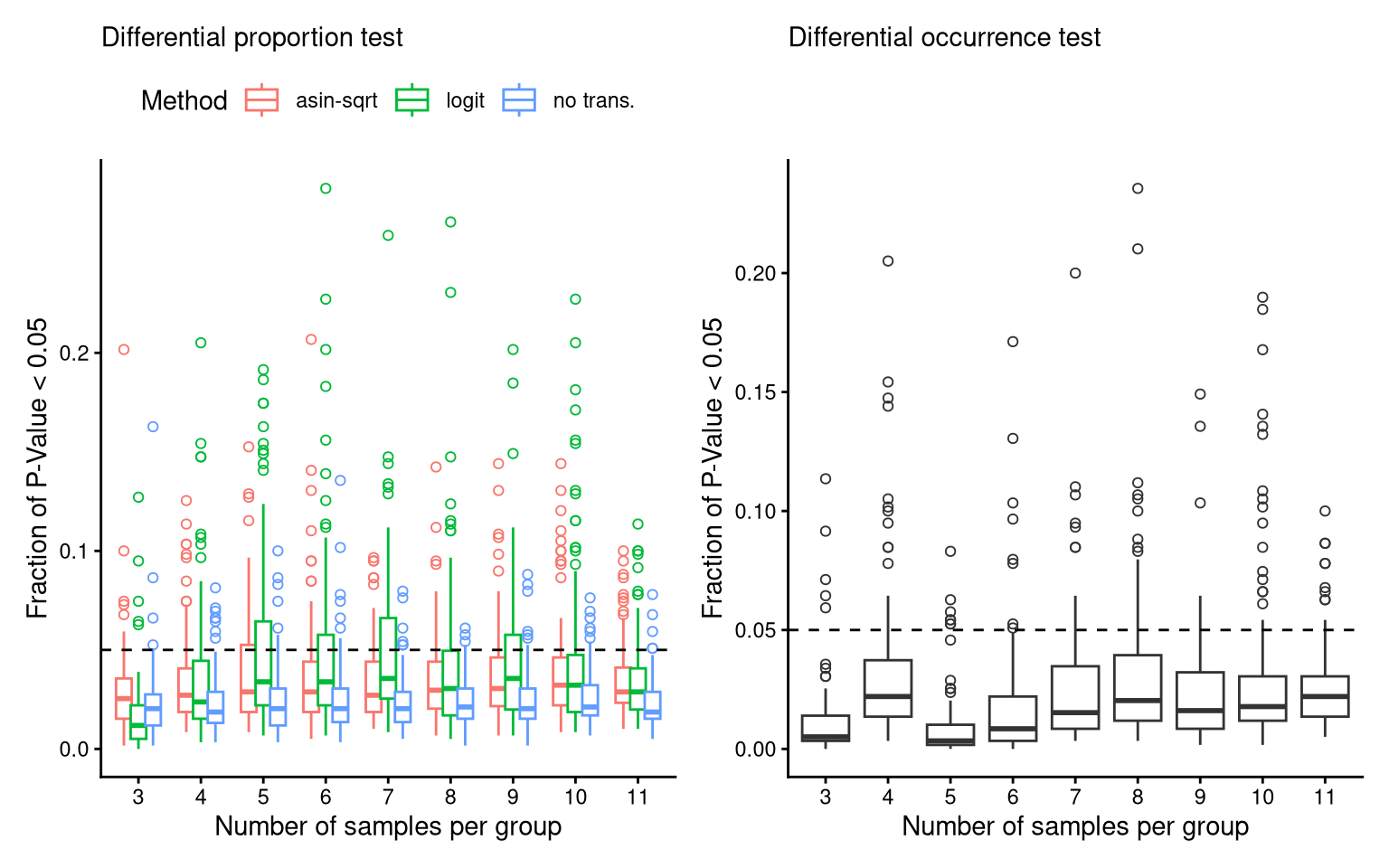

P_FPR_C22

Ignoring unknown labels:
• titlte : ""

Warning: No shared levels found between `names(values)` of the manual scale and the
data's colour values.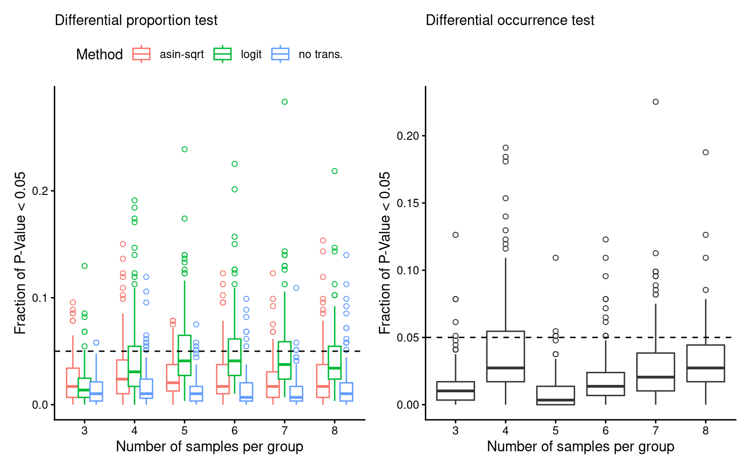

P_FPR_C23

Ignoring unknown labels:
• titlte : ""

Warning: No shared levels found between `names(values)` of the manual scale and the
data's colour values.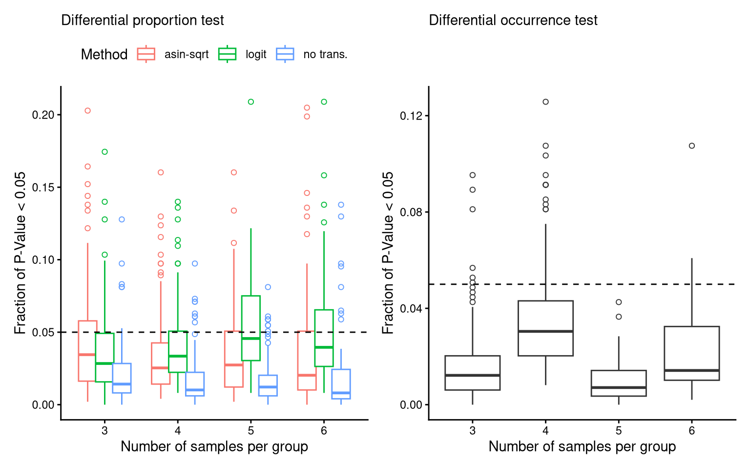

9 Figure S2-HSPC xenograft

layout = "
ABB
CDD
EFF
"
fs2_xeno <- (
    wrap_elements(p_prop_C21 + theme(plot.margin = unit(c(0,0,0,0), "line"))) + 
  wrap_elements(P_FPR_C21 + theme(legend.position = "top") + theme(plot.margin = unit(rep(0,4), "cm"))) + 
    wrap_elements(p_prop_C22 + theme(plot.margin = unit(c(0,0,0,0), "line"))) + 
  wrap_elements(P_FPR_C22 + theme(legend.position = "top") + theme(plot.margin = unit(rep(0,4), "cm"))) + 
    wrap_elements(p_prop_C23 + theme(plot.margin = unit(c(0,0,0,0), "line"))) + 
  wrap_elements(P_FPR_C23 + theme(legend.position = "top") + theme(plot.margin = unit(rep(0,4), "cm")))
) + 
  plot_layout(design = layout) +
  plot_annotation(tag_levels = list(c("A", "B", "C", "D", "E", "F"))) &
  theme(
    plot.tag = element_text(size = 20, face = "bold", family = "arial"),
    axis.title = element_text(size = 17),
    axis.text = element_text(size = 12),
    legend.title = element_text(size = 13),
    legend.text = element_text(size = 11))

fs2_xeno

Ignoring unknown labels:
• titlte : ""

Warning: No shared levels found between `names(values)` of the manual scale and the
data's colour values.

Ignoring unknown labels:
• titlte : ""

Warning: No shared levels found between `names(values)` of the manual scale and the
data's colour values.

Ignoring unknown labels:
• titlte : ""

Warning: No shared levels found between `names(values)` of the manual scale and the
data's colour values.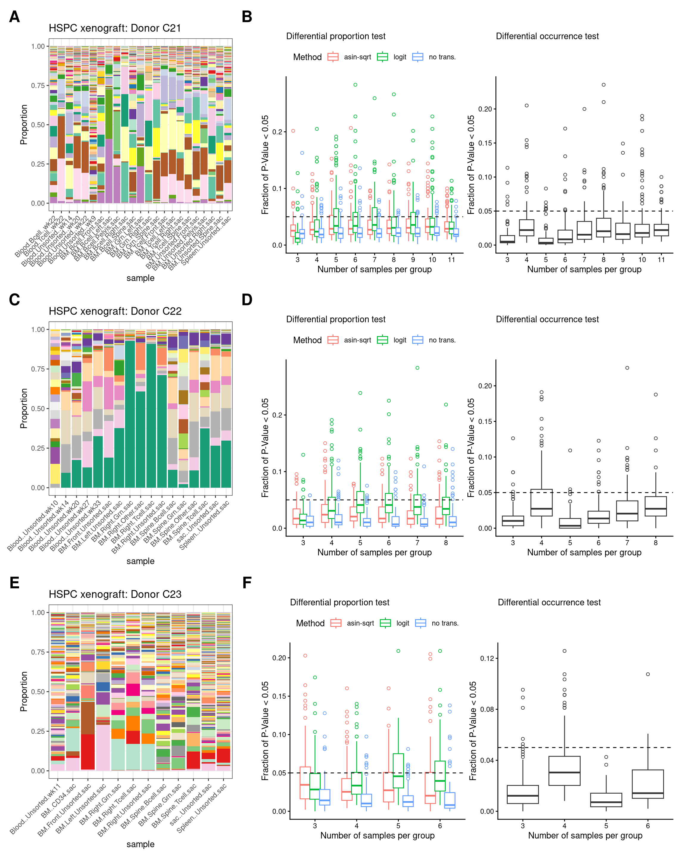

ggsave(
  filename = "output/fs2_xeno.png",
  plot = fs2_xeno,
  width = 12,
  height = 15,
  units = "in", # for Rmd r chunk fig size, unit default to inch
  dpi = 350
  )

Ignoring unknown labels:
• titlte : ""

Warning: No shared levels found between `names(values)` of the manual scale and the
data's colour values.

Ignoring unknown labels:
• titlte : ""

Warning: No shared levels found between `names(values)` of the manual scale and the
data's colour values.

Ignoring unknown labels:
• titlte : ""

Warning: No shared levels found between `names(values)` of the manual scale and the
data's colour values.

Saving this figure in fs2_xenoHSPC

sessionInfo()

R version 4.5.0 (2025-04-11)
Platform: x86_64-pc-linux-gnu
Running under: Red Hat Enterprise Linux 9.6 (Plow)

Matrix products: default
BLAS/LAPACK: FlexiBLAS OPENBLAS-OPENMP;  LAPACK version 3.9.0

locale:
 [1] LC_CTYPE=en_AU.UTF-8       LC_NUMERIC=C              
 [3] LC_TIME=en_AU.UTF-8        LC_COLLATE=en_AU.UTF-8    
 [5] LC_MONETARY=en_AU.UTF-8    LC_MESSAGES=en_AU.UTF-8   
 [7] LC_PAPER=en_AU.UTF-8       LC_NAME=C                 
 [9] LC_ADDRESS=C               LC_TELEPHONE=C            
[11] LC_MEASUREMENT=en_AU.UTF-8 LC_IDENTIFICATION=C       

time zone: Australia/Melbourne
tzcode source: system (glibc)

attached base packages:
[1] stats4    grid      stats     graphics  grDevices utils     datasets 
[8] methods   base     

other attached packages:
 [1] barbieQ_1.1.3               devtools_2.4.6             
 [3] usethis_3.2.1               SEtools_1.22.0             
 [5] sechm_1.16.0                SummarizedExperiment_1.38.1
 [7] Biobase_2.68.0              GenomicRanges_1.60.0       
 [9] GenomeInfoDb_1.44.3         IRanges_2.42.0             
[11] S4Vectors_0.48.0            BiocGenerics_0.54.0        
[13] generics_0.1.4              MatrixGenerics_1.20.0      
[15] matrixStats_1.5.0           edgeR_4.6.3                
[17] limma_3.64.3                ComplexHeatmap_2.24.1      
[19] ggVennDiagram_1.5.4         scales_1.4.0               
[21] patchwork_1.3.2             ggplot2_4.0.0              
[23] knitr_1.50                  tibble_3.3.0               
[25] tidyr_1.3.1                 dplyr_1.1.4                
[27] magrittr_2.0.4              readxl_1.4.5               
[29] workflowr_1.7.2            

loaded via a namespace (and not attached):
  [1] splines_4.5.0           later_1.4.4             ggplotify_0.1.3        
  [4] cellranger_1.1.0        polyclip_1.10-7         rpart_4.1.24           
  [7] XML_3.99-0.20           lifecycle_1.0.4         Rdpack_2.6.4           
 [10] formula.tools_1.7.1     doParallel_1.0.17       rprojroot_2.1.1        
 [13] processx_3.8.6          lattice_0.22-6          MASS_7.3-65            
 [16] backports_1.5.0         openxlsx_4.2.8.1        sass_0.4.10            
 [19] rmarkdown_2.30          jquerylib_0.1.4         yaml_2.3.10            
 [22] remotes_2.5.0           httpuv_1.6.16           zip_2.3.3              
 [25] sessioninfo_1.2.3       pkgbuild_1.4.8          minqa_1.2.8            
 [28] DBI_1.2.3               RColorBrewer_1.1-3      abind_1.4-8            
 [31] pkgload_1.4.1           Rtsne_0.17              purrr_1.1.0            
 [34] ggraph_2.2.2            nnet_7.3-20             yulab.utils_0.2.1      
 [37] tweenr_2.0.3            rappdirs_0.3.3          git2r_0.36.2           
 [40] sva_3.56.0              circlize_0.4.16         seriation_1.5.8        
 [43] GenomeInfoDbData_1.2.14 ggrepel_0.9.6           genefilter_1.90.0      
 [46] pheatmap_1.0.13         annotate_1.86.1         codetools_0.2-20       
 [49] DelayedArray_0.34.1     ggforce_0.5.0           tidyselect_1.2.1       
 [52] shape_1.4.6.1           aplot_0.2.9             UCSC.utils_1.4.0       
 [55] farver_2.1.2            lme4_1.1-37             viridis_0.6.5          
 [58] TSP_1.2.6               jsonlite_2.0.0          GetoptLong_1.0.5       
 [61] mitml_0.4-5             ellipsis_0.3.2          tidygraph_1.3.1        
 [64] ggbreak_0.1.6           randomcoloR_1.1.0.1     survival_3.8-3         
 [67] iterators_1.0.14        systemfonts_1.3.1       foreach_1.5.2          
 [70] tools_4.5.0             ragg_1.5.0              Rcpp_1.1.0             
 [73] glue_1.8.0              pan_1.9                 gridExtra_2.3          
 [76] SparseArray_1.8.1       xfun_0.53               mgcv_1.9-1             
 [79] DESeq2_1.48.2           logistf_1.26.1          ca_0.71.1              
 [82] withr_3.0.2             fastmap_1.2.0           boot_1.3-31            
 [85] callr_3.7.6             digest_0.6.37           R6_2.6.1               
 [88] gridGraphics_0.5-1      textshaping_1.0.3       mice_3.18.0            
 [91] colorspace_2.1-2        RSQLite_2.4.5           data.table_1.17.8      
 [94] graphlayouts_1.2.2      httr_1.4.7              S4Arrays_1.8.1         
 [97] whisker_0.4.1           pkgconfig_2.0.3         gtable_0.3.6           
[100] blob_1.2.4              registry_0.5-1          S7_0.2.0               
[103] XVector_0.48.0          htmltools_0.5.8.1       clue_0.3-66            
[106] png_0.1-8               reformulas_0.4.1        ggfun_0.2.0            
[109] rstudioapi_0.17.1       rjson_0.2.23            nloptr_2.2.1           
[112] nlme_3.1-168            curl_7.0.0              cachem_1.1.0           
[115] GlobalOptions_0.1.2     stringr_1.5.2           operator.tools_1.6.3   
[118] parallel_4.5.0          AnnotationDbi_1.70.0    pillar_1.11.1          
[121] vctrs_0.6.5             promises_1.3.3          jomo_2.7-6             
[124] xtable_1.8-4            cluster_2.1.8.1         evaluate_1.0.5         
[127] magick_2.9.0            cli_3.6.5               locfit_1.5-9.12        
[130] compiler_4.5.0          rlang_1.1.6             crayon_1.5.3           
[133] labeling_0.4.3          ps_1.9.1                getPass_0.2-4          
[136] fs_1.6.6                stringi_1.8.7           viridisLite_0.4.2      
[139] BiocParallel_1.42.2     Biostrings_2.76.0       glmnet_4.1-10          
[142] V8_8.0.1                Matrix_1.7-3            bit64_4.6.0-1          
[145] KEGGREST_1.48.1         statmod_1.5.0           rbibutils_2.3          
[148] broom_1.0.10            igraph_2.1.4            memoise_2.0.1          
[151] bslib_0.9.0             bit_4.6.0

barbieQ_paper Supplementary 2: Type I error rate using `HSPC xenograft data`

Liyang Fei

Initiated: 2025-04-11 Rendered: 2026-01-07

1 Load Dependencies

2 Install `barbieQ`

3 Set seeds

4 Load preprocessed data

5 Samples level QC

5.1 PCA

5.2 Plot propportion

5.3 Heatmap

6 Subset samples of indivisual donors

6.1 Donor C21

6.2 Donor C22

6.3 Donor C23

7 Plot proportion

7.1 Donor C21

7.2 Donor C22

7.3 Donor C23

7.4 FS2A,C,E: prop. of three donors

8 Type I error rate

8.1 Donor C21

8.2 Donor C22

8.3 Donor C23

8.4 FS2B,D,F: FPR of three donors

9 Figure S2-HSPC xenograft

barbieQ_paper Supplementary 2: Type I error rate using HSPC xenograft data

Liyang Fei

Initiated: 2025-04-11 Rendered: 2026-01-07

1 Load Dependencies

2 Install barbieQ

3 Set seeds

4 Load preprocessed data

5 Samples level QC

5.1 PCA

5.2 Plot propportion

5.3 Heatmap

6 Subset samples of indivisual donors

6.1 Donor C21

6.2 Donor C22

6.3 Donor C23

7 Plot proportion

7.1 Donor C21

7.2 Donor C22

7.3 Donor C23

7.4 FS2A,C,E: prop. of three donors

8 Type I error rate

8.1 Donor C21

8.2 Donor C22

8.3 Donor C23

8.4 FS2B,D,F: FPR of three donors

9 Figure S2-HSPC xenograft

barbieQ_paper Supplementary 2: Type I error rate using `HSPC xenograft data`

2 Install `barbieQ`