Combined Figures
Last updated: 2019-01-07
workflowr checks: (Click a bullet for more information)-
✔ R Markdown file: up-to-date
Great! Since the R Markdown file has been committed to the Git repository, you know the exact version of the code that produced these results.
-
✔ Environment: empty
Great job! The global environment was empty. Objects defined in the global environment can affect the analysis in your R Markdown file in unknown ways. For reproduciblity it’s best to always run the code in an empty environment.
-
✔ Seed:
set.seed(20180730)The command
set.seed(20180730)was run prior to running the code in the R Markdown file. Setting a seed ensures that any results that rely on randomness, e.g. subsampling or permutations, are reproducible. -
✔ Session information: recorded
Great job! Recording the operating system, R version, and package versions is critical for reproducibility.
-
Great! You are using Git for version control. Tracking code development and connecting the code version to the results is critical for reproducibility. The version displayed above was the version of the Git repository at the time these results were generated.✔ Repository version: 182dd0e
Note that you need to be careful to ensure that all relevant files for the analysis have been committed to Git prior to generating the results (you can usewflow_publishorwflow_git_commit). workflowr only checks the R Markdown file, but you know if there are other scripts or data files that it depends on. Below is the status of the Git repository when the results were generated:
Note that any generated files, e.g. HTML, png, CSS, etc., are not included in this status report because it is ok for generated content to have uncommitted changes.Ignored files: Ignored: .DS_Store Ignored: .Rhistory Ignored: .Rproj.user/ Ignored: analysis/cache.bak.20181031/ Ignored: analysis/cache.bak/ Ignored: analysis/cache.lind2.20181114/ Ignored: analysis/cache/ Ignored: data/Lindstrom2/ Ignored: data/processed.bak.20181031/ Ignored: data/processed.bak/ Ignored: data/processed.lind2.20181114/ Ignored: packrat/lib-R/ Ignored: packrat/lib-ext/ Ignored: packrat/lib/ Ignored: packrat/src/ Ignored: test.csv.zip Unstaged changes: Modified: output/07D_Combined_Figures/figure3F.pdf Modified: output/07D_Combined_Figures/figure3_panel.pdf
Expand here to see past versions:
| File | Version | Author | Date | Message |
|---|---|---|---|---|
| Rmd | 182dd0e | Luke Zappia | 2019-01-07 | Adjust Fig 3F gene list |
| html | 858cf44 | Luke Zappia | 2018-12-04 | Add hFK podocyte DE |
| Rmd | 2f21982 | Luke Zappia | 2018-12-04 | Minor updates to figures |
| Rmd | 1b1ce1c | Luke Zappia | 2018-11-23 | Update gene lists for figures |
| html | 1b1ce1c | Luke Zappia | 2018-11-23 | Update gene lists for figures |
| Rmd | 292a1c6 | Luke Zappia | 2018-11-23 | Minor fixes to output |
| html | 292a1c6 | Luke Zappia | 2018-11-23 | Minor fixes to output |
| Rmd | a1f9f38 | Luke Zappia | 2018-11-23 | Revise figures |
| html | a1f9f38 | Luke Zappia | 2018-11-23 | Revise figures |
| html | 2354d70 | Luke Zappia | 2018-09-13 | Tidy output files |
| html | a61f9c9 | Luke Zappia | 2018-09-13 | Rebuild site |
| html | ad10b21 | Luke Zappia | 2018-09-13 | Switch to GitHub |
| Rmd | ff4bd7c | Luke Zappia | 2018-09-13 | Rename proximal early nephron clusters |
| Rmd | 1d8b5a6 | Luke Zappia | 2018-09-11 | Update methods |
| Rmd | 91342d1 | Luke Zappia | 2018-09-10 | Adjust colours and remove shadows |
| Rmd | 35d26cc | Luke Zappia | 2018-09-10 | Update Figure 2E gene list |
| Rmd | c30f923 | Luke Zappia | 2018-09-07 | Add combined figures |
# scRNA-seq
library("Seurat")
library("monocle")

# Plotting
library("clustree")
library("cowplot")

# Presentation
library("glue")
library("knitr")

# Parallel

# Paths
library("here")

# Output

# Tidyverse
library("tidyverse")
source(here("R/output.R"))
source(here("R/crossover.R"))comb.path <- here("data/processed/Combined_clustered.Rds")
comb.neph.path <- here("data/processed/Combined_nephron.Rds")
o.path <- here("output/04_Organoids_Clustering/cluster_assignments.csv")
on.path <- here("output/04B_Organoids_Nephron/cluster_assignments.csv")
c.path <- here("output/07_Combined_Clustering/cluster_assignments.csv")
cn.path <- here("output/07B_Combined_Nephron/cluster_assignments.csv")
dir.create(here("output", DOCNAME), showWarnings = FALSE)Introduction
In this document we are going to look at all of the organoids analysis results and produce a series of figures for the paper.
if (file.exists(comb.path)) {
    comb <- read_rds(comb.path)
} else {
    stop("Clustered Combined dataset is missing. ",
         "Please run '07_Combined_Clustering.Rmd' first.",
         call. = FALSE)
}
if (file.exists(comb.neph.path)) {
comb.neph <- read_rds(comb.neph.path)
} else {
stop("Clustered Combined nephron dataset is missing. ",
"Please run '07B_Organoids_Nephron.Rmd' first.",
call. = FALSE)
}orgs.clusts <- read_csv(o.path,
col_types = cols(
Cell = col_character(),
Dataset = col_character(),
Sample = col_integer(),
Barcode = col_character(),
Cluster = col_integer()
)) %>%
rename(Organoids = Cluster)
orgs.neph.clusts <- read_csv(on.path,
col_types = cols(
Cell = col_character(),
Dataset = col_character(),
Sample = col_integer(),
Barcode = col_character(),
Cluster = col_integer()
)) %>%
rename(OrgsNephron = Cluster)
comb.clusts <- read_csv(c.path,
col_types = cols(
Cell = col_character(),
Dataset = col_character(),
Sample = col_integer(),
Barcode = col_character(),
Cluster = col_integer()
)) %>%
rename(Combined = Cluster)
comb.neph.clusts <- read_csv(cn.path,
col_types = cols(
Cell = col_character(),
Dataset = col_character(),
Sample = col_integer(),
Barcode = col_character(),
Cluster = col_integer()
)) %>%
rename(CombNephron = Cluster)
clusts <- comb.clusts %>%
left_join(comb.neph.clusts,
by = c("Cell", "Dataset", "Sample", "Barcode")) %>%
left_join(orgs.clusts,
by = c("Cell", "Dataset", "Sample", "Barcode")) %>%
left_join(orgs.neph.clusts,
by = c("Cell", "Dataset", "Sample", "Barcode"))Figure 2
Figure 2A
plot.data <- comb %>%
    GetDimReduction("tsne",  slot = "cell.embeddings") %>%
    data.frame() %>%
    rownames_to_column("Cell") %>%
    mutate(Group = comb@meta.data$Group) %>%
    mutate(Group = if_else(Group == "Lindstrom", "Fetal kidney", Group)) %>%
    mutate(Cluster = comb@ident)

f2A <- ggplot(plot.data, aes(x = tSNE_1, y = tSNE_2, colour = Group)) +
    geom_point() +
    scale_color_manual(values = c("#EC008C", "#00ADEF")) +
    guides(colour = guide_legend(ncol = 1,
                                 override.aes = list(size = 10))) +
    theme_cowplot() +
    theme(legend.position = "bottom",
          legend.title = element_blank(),
          legend.justification = "center")

ggsave(here("output", DOCNAME, "figure2A.png"), f2A,
       height = 8, width = 10)
ggsave(here("output", DOCNAME, "figure2A.pdf"), f2A,
       height = 8, width = 10)

f2A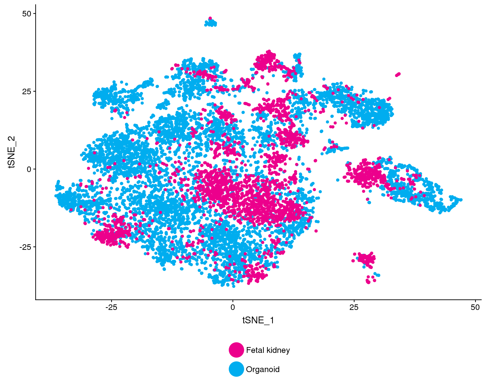
Expand here to see past versions of fig-2A-1.png:
| Version | Author | Date |
|---|---|---|
| ad10b21 | Luke Zappia | 2018-09-13 |
Figure 2B
lab.data <- plot.data %>%
    group_by(Cluster) %>%
    summarise(tSNE_1 = mean(tSNE_1),
              tSNE_2 = mean(tSNE_2)) %>%
    mutate(Label = paste0("C", Cluster))

clust.labs <- c(
    "C0 (Stroma)\nTAGLN, ALDH1A2, COL6A3",
    "C1 (Stroma)\nDCN, LUM, POSTN",
    "C2 (Stroma)\nMGP, GATA3, NDUFA4L2",
    "C3 (Stroma)\nZFHX4, CTSK, HNRNPA1",
    "C4 (Endothelium)\nGNG11, CLDN5, CD34",
    "C5 (Cell cycle)\nHIST1H4C, PCLAF, DUT",
    "C6 (Committing nephron prog.)\nLYPD1, DAPL1, PAX8",
    "C7 (Podocyte)\nPODXL, MAFB, TCF21",
    "C8 (Cell cycle)\nCENPF, HMGB2, UBE2C",
    "C9 (Stroma)\nCOL9A3, FIBIN, DLK1",
    "C10 (Nephron)\nIGFBP7, EMBX2, MAL",
    "C11 (Glial)\nTTYH1, FABP7, SOX2",
    "C12 (Immune)\nPTPRC, TYROBP, FCER1G",
    "C13 (Blood)\nHBG1, HBB, HBA2",
    "C14 (Neural prog.)\nSOX11, ELAVL3, ELAVL4",
    "C15 (Podocyte)\nPTPRO, TCF21, PODXL"
)

f2B <- ggplot(plot.data, aes(x = tSNE_1, y = tSNE_2, colour = Cluster)) +
    geom_point() +
    geom_text(data = lab.data, aes(label = Label), colour = "black", size = 8) +
    scale_colour_discrete(labels = clust.labs) +
    guides(colour = guide_legend(nrow = 3, override.aes = list(size = 10),
                                 label.theme = element_text(size = 10))) +
    theme_cowplot() +
    theme(legend.position = "bottom",
          legend.title = element_blank(),
          legend.justification = "center")

ggsave(here("output", DOCNAME, "figure2B.png"), f2B,
       height = 8, width = 10)
ggsave(here("output", DOCNAME, "figure2B.pdf"), f2B,
       height = 8, width = 10)

f2B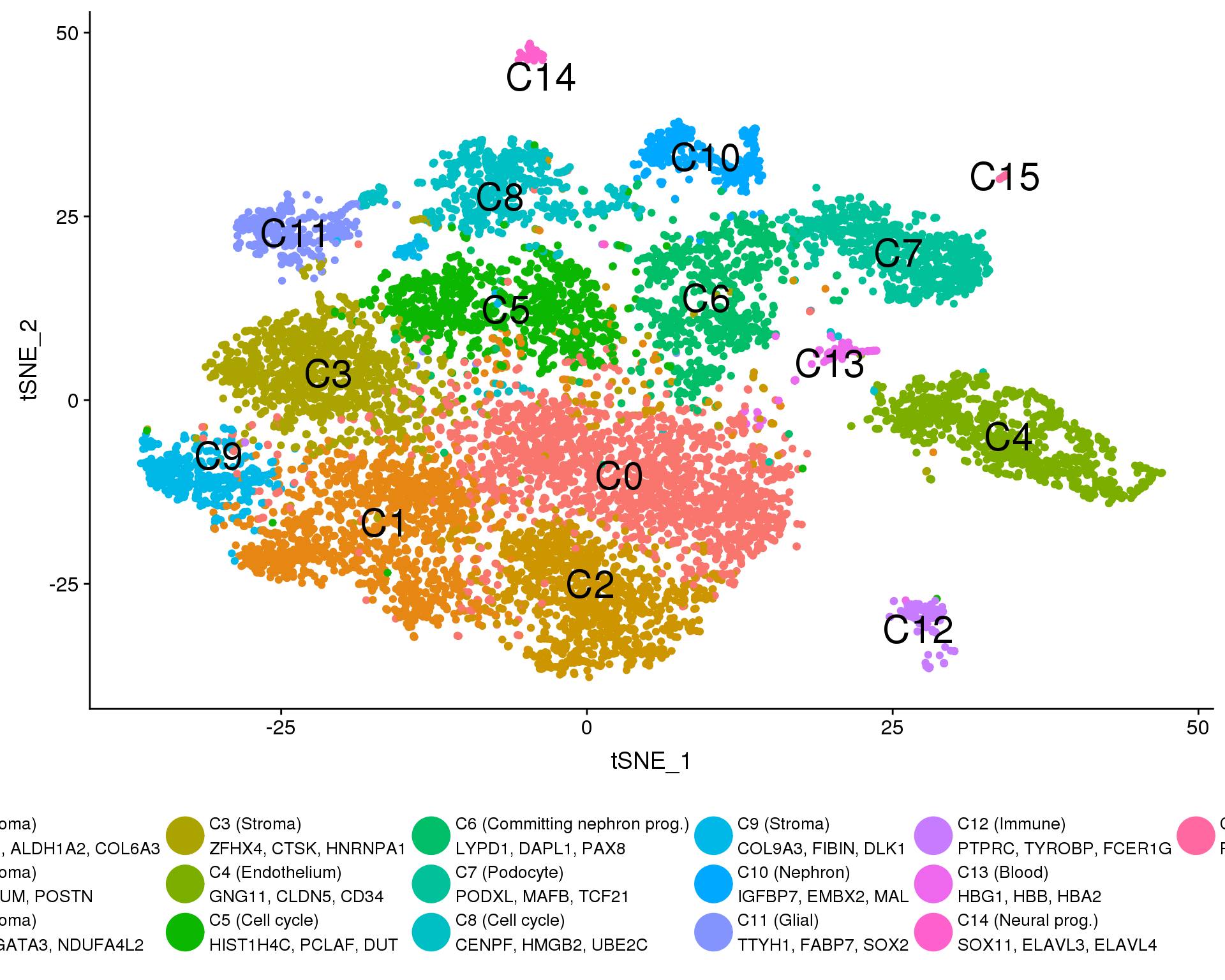
Figure 2AB legend
l2A <- get_legend(f2A)
l2B <- get_legend(f2B)

l2AB <- plot_grid(l2A, l2B, nrow = 1, rel_widths = c(0.15, 1))

l2AB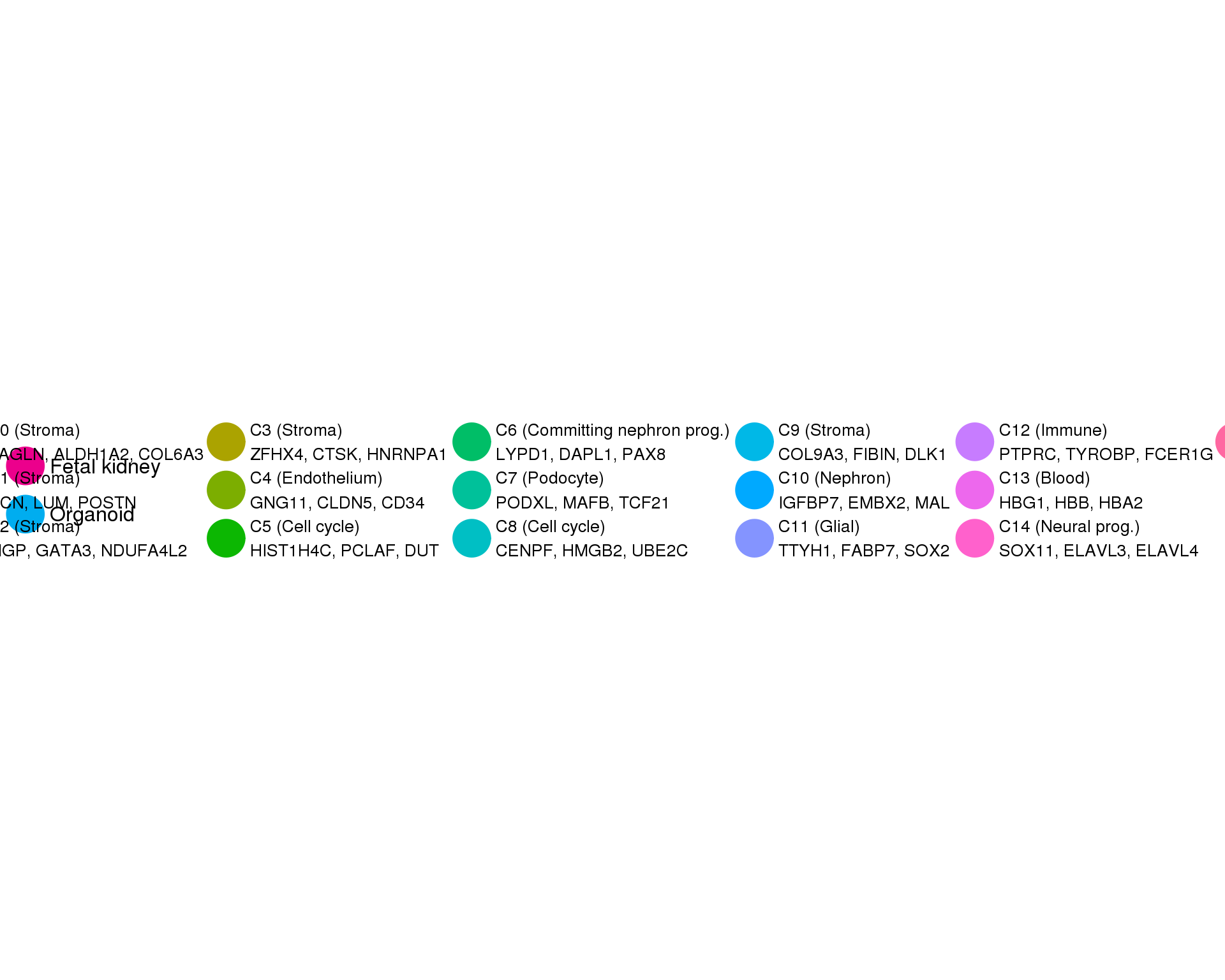
Figure 2C
f2C <- summariseClusts(clusts, Combined, Organoids) %>%
    replace_na(list(Jaccard = 0)) %>%
    ggplot(aes(x = Combined, y = Organoids, fill = Jaccard)) +
    geom_tile() +
    scale_fill_viridis_c(limits = c(0, 1), name = "Jaccard\nindex") +
    scale_x_discrete(labels = paste0("C", 0:15)) +
    scale_y_discrete(labels = paste0("O", 0:12)) +
    coord_equal() +
    xlab("Combined clusters") +
    ylab("Organoid clusters") +
    theme_minimal() +
    theme(axis.text = element_text(size = 10, colour = "black"),
          axis.ticks = element_blank(),
          axis.title = element_text(size = 15),
          legend.key.height = unit(30, "pt"),
          legend.title = element_text(size = 15),
          legend.text = element_text(size = 10),
          panel.grid = element_blank())

ggsave(here("output", DOCNAME, "figure2C.png"), f2C,
       height = 8, width = 10)
ggsave(here("output", DOCNAME, "figure2C.pdf"), f2C,
       height = 8, width = 10)

f2C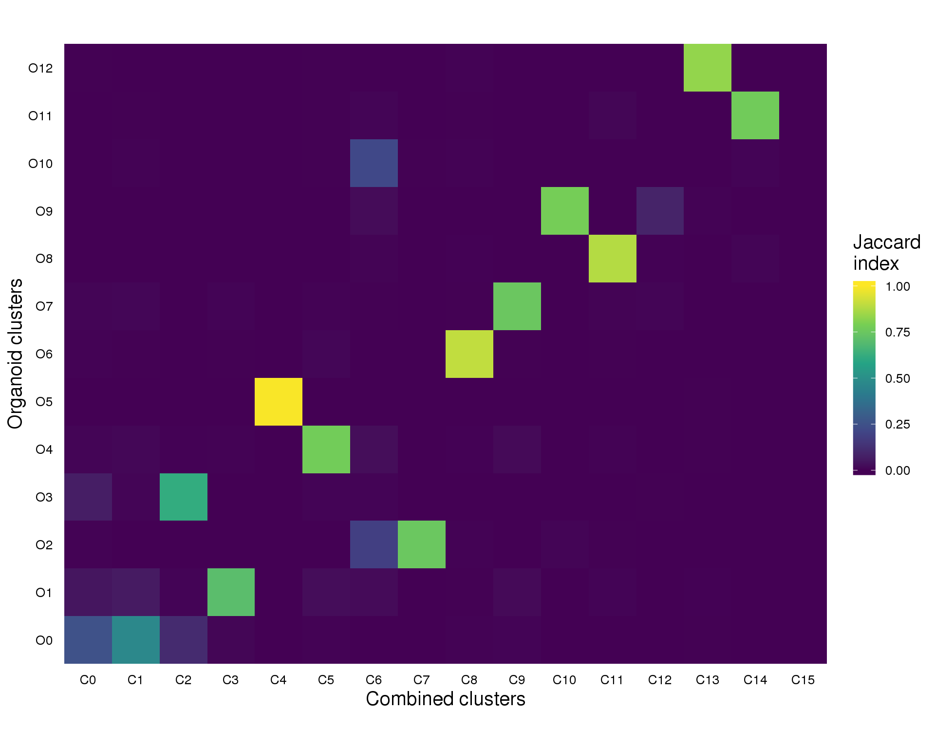
Figure 2D
labs <- paste0("C", 0:max(as.numeric(comb@meta.data$Cluster)))

plot.data <- comb@meta.data %>%
    select(Cluster, Group) %>%
    mutate(Cluster = paste0("C", Cluster)) %>%
    mutate(Cluster = factor(Cluster, levels = labs)) %>%
    mutate(Group = if_else(Group == "Lindstrom", "Fetal kidney", Group))

f2D <- ggplot(plot.data, aes(x = Cluster, fill = Cluster)) +
    geom_bar() +
    labs(y = "Number of cells") +
    facet_wrap(~ Group, ncol = 1, scales = "free_y") +
    theme_cowplot() +
    theme(legend.position = "none",
          axis.title.x = element_blank(),
          axis.text = element_text(size = 10),
          strip.text = element_text(size = 15,
                                    margin = margin(0, 0, 2, 0, "pt")),
          strip.background = element_blank(),
          strip.placement = "outside")

ggsave(here("output", DOCNAME, "figure2D.png"), f2D,
       height = 8, width = 10)
ggsave(here("output", DOCNAME, "figure2D.pdf"), f2D,
       height = 8, width = 10)

f2D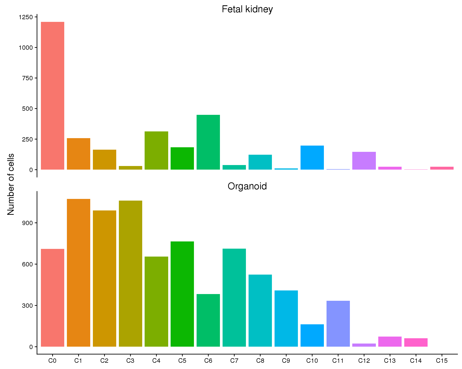
Figure 2E
plot.data <- comb@meta.data %>%
    select(Cluster, Group) %>%
    mutate(Tissue = fct_collapse(Cluster,
                                 Stroma = c("0", "1", "2", "3", "9"),
                                 Nephron = c("6", "7", "10", "15"),
                                 Endothelial = c("4"),
                                 `Cell cycle` = c("5", "8"),
                                 Other = c("11", "12", "13", "14"))) %>%
    mutate(Tissue = fct_relevel(Tissue,
                                "Stroma", "Nephron", "Endothelial",
                                "Cell cycle", "Other")) %>%
    group_by(Group, Tissue) %>%
    summarise(Count = n()) %>%
    mutate(Prop = Count / sum(Count)) %>%
    ungroup() %>%
    mutate(Group = if_else(Group == "Lindstrom", "Fetal kidney", Group))

f2E <- ggplot(plot.data, aes(x = Group, y = Prop, fill = Tissue)) +
    geom_col() +
    labs(y = "Proportion of cells") +
    guides(fill = guide_legend(direction = "vertical", ncol = 2)) +
    theme_cowplot() +
    theme(axis.title.x = element_blank(),
          legend.title = element_blank(),
          legend.position = "bottom")

ggsave(here("output", DOCNAME, "figure2E.png"), f2E,
       height = 8, width = 10)
ggsave(here("output", DOCNAME, "figure2E.pdf"), f2E,
       height = 8, width = 10)

f2E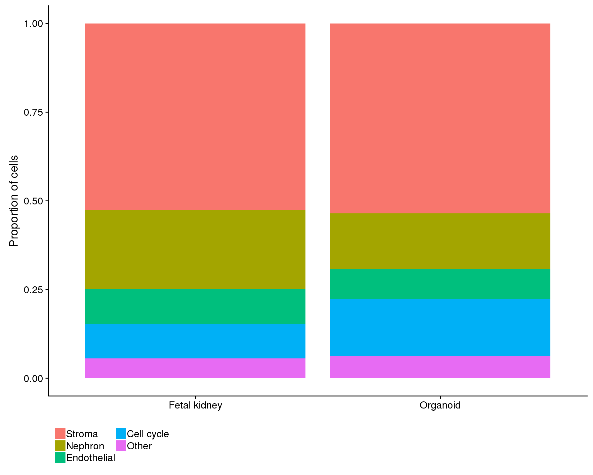
Figure 2F
genes <- c("HSPA1A", "HSPA1B", "HBG2", "HSP90AA1", "DNAJB1", "FOS", "HSPA6",
           "HBG1", "JUN", "GPC3", "MARCKSL1", "MARCKS", "RPS26", "YBX1",
           "HMGN2", "EEF1A1", "RPL41", "RPL39", "H3F3A", "RPS17")

gene.groups <- c(rep("Up-regulated in fetal kidney", 10),
                 rep("Up-regulated in organoid", 10)) %>%
    fct_relevel("Up-regulated in fetal kidney", "Up-regulated in organoid")
names(gene.groups) <- genes

group.labs <- c("Fetal kidney", "Organoid")

plot.data <- data.frame(FetchData(comb.neph, vars.all = genes)) %>%
    rownames_to_column("Cell") %>%
    mutate(Group = comb.neph@meta.data$Group) %>%
    gather(key = "Gene", value = "Expr", -Cell, -Group) %>%
    group_by(Group, Gene) %>%
    summarize(AvgExpr = mean(expm1(Expr)),
              PctExpr = Seurat:::PercentAbove(Expr, threshold = 0) * 100) %>%
    group_by(Gene) %>%
    mutate(AvgExprScale = scale(AvgExpr)) %>%
    mutate(AvgExprScale = Seurat::MinMax(AvgExprScale,
                                         max = 2.5, min = -2.5)) %>%
    ungroup() %>%
    mutate(GeneGroup = gene.groups[Gene]) %>%
    mutate(Gene = factor(Gene, levels = genes))

f2F <- ggplot(plot.data,
              aes(x = Gene, y = Group, size = PctExpr,
                  colour = Group, alpha = AvgExprScale)) +
       geom_point() +
       scale_radius(range = c(0, 10)) +
       scale_color_manual(values = c("#EC008C", "#00ADEF")) +
       scale_y_discrete(labels = group.labs) +
       facet_grid(~ GeneGroup, scales = "free_x") +
       theme(axis.title.x = element_blank(),
             axis.title.y = element_blank(),
             axis.text.x = element_text(angle = 90, vjust = 0.5, hjust = 1),
             panel.spacing = unit(x = 1, units = "lines"),
             strip.background = element_blank(),
             strip.placement = "outside",
             strip.text = element_text(size = 15,
                                       margin = margin(0, 0, 2, 0, "pt")),
             legend.position = "none")

ggsave(here("output", DOCNAME, "figure2F.png"), f2F,
       height = 8, width = 10)
ggsave(here("output", DOCNAME, "figure2F.pdf"), f2F,
       height = 8, width = 10)

f2F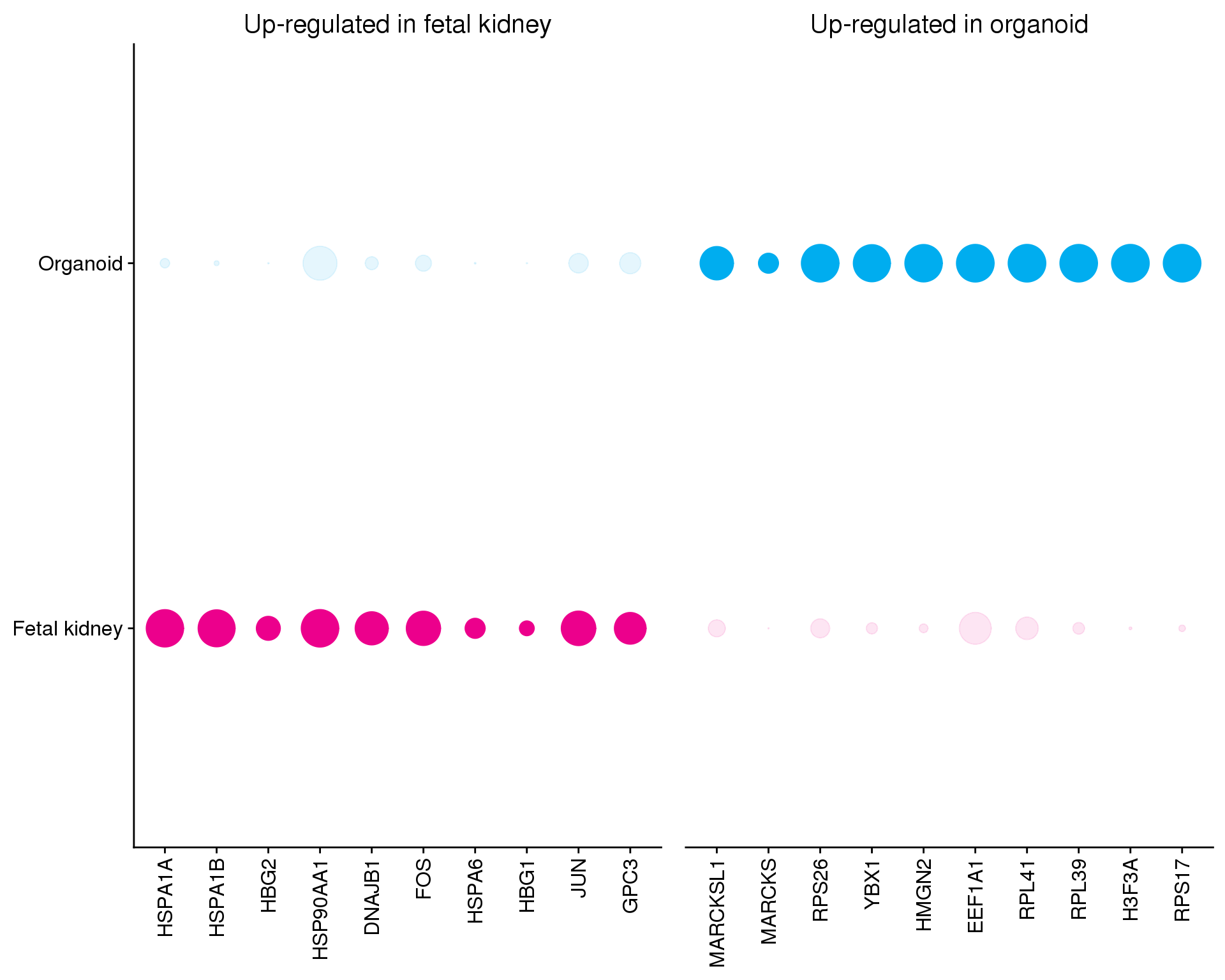
Expand here to see past versions of fig-2F-1.png:
| Version | Author | Date |
|---|---|---|
| a1f9f38 | Luke Zappia | 2018-11-23 |
Figure 2G
genes.list <- list(
    `0` = c("GPC3", "SULT1E1", "CCBE1", "LBH", "CKS2", "STMN2", "NRK", "ACTA2",
            "PDGFRA", "ALX1", "COL6A3", "ALDH1A2", "TAGLN"),
    `1` = c("DKK2", "WNT2B", "S100A10", "SERPINI1", "PALLD", "DKK1", "ACTA2_1",
            "SFRP2", "POSTN", "IGF1", "LUM", "COL1A1", "DCN"),
    `2` = c("ANGPT2", "MCAM", "TUBA1B", "ENG", "ID1", "REN", "FTL", "SSBP4",
            "PDLIM1", "MEF2C", "PDGFRB", "GATA3", "MGP"),
    `3` = c("ROBO2", "ANGPT1", "NR2F1", "ACTA2_2", "SNHG8", "DKK1_1", "VAMP2",
            "VIM", "TBX3", "SOX4", "HNRNPA1", "CTSK", "ZFHX4"),
    `9` = c("IGF1_1", "ITM2B", "PLPP3", "COL1A1_1", "COL11A1", "COL9A1",
            "PEG10", "CNMD", "OGN", "FIBIN", "LUM_1", "DCN_1", "COL9A3"),
    `4` = c("CXCL8", "CXCL1", "CXCL2", "ICAM1", "HEY1", "CXCR4", "APLN",
            "PECAM1", "PLXND1", "CD34", "ESAM", "CLDN5", "GNG11"),
    `11` = c("PMP22", "MPZ", "ERBB3", "ARHGAP15", "MSX1", "ZFP36L1", "FABP7",
             "AP1S2", "VIM_1", "SOX2", "PLP1", "TTYH1", "S100B"),
    `14` = c("STMN1", "NCAM1", "RBP1", "ATOH1", "ELAVL4", "SOX11", "ELAVL3",
             "DCX", "TUBA1A", "STMN2_1", "CRABP1", "TUBB2B", "HES6"),
    `12` = c("CXCL8_1", "IL1B", "HLA-DPA1", "HLA-DPB1", "LGALS1", "CTSG", "MPO",
             "PRTN3", "TYROBP", "S100A9", "SRGN", "CD74", "PTPRC"),
    `13` = c("HBA1", "HBA2", "HBB", "HBG1", "AHSP", "HBM", "GNG5", "EGFL7",
             "FSCN1", "FKBP1A", "GPX1", "SLC25A3", "GYPC")
)

clust.labs <- c("C0\nStr", "C1\nStr", "C2\nStr", "C3\nStr", "C9\nStr",
                "C4\nEndo", "C11\nGlia", "C14\nNeural", "C12\nImmune",
                "C13\nBlood")

plot.data <- lapply(names(genes.list), function(name) {
    genes.raw <- genes.list[[name]]
    genes <- str_remove(genes.raw, "_[0-9]")
    names(genes.raw) <- genes
    comb %>%
        FetchData(vars.all = genes) %>%
        as_data_frame() %>%
        rownames_to_column("Cell") %>%
        mutate(Cluster = as.numeric(as.character(comb@ident)),
               Group = comb@meta.data$Group) %>%
        gather(key = "Gene", value = "Expr", -Cell, -Cluster, -Group) %>%
        group_by(Cluster, Gene, Group) %>%
        summarize(AvgExpr = mean(expm1(Expr)),
                  PctExpr = Seurat:::PercentAbove(Expr, threshold = 0) * 100) %>%
        group_by(Gene) %>%
        mutate(AvgExprScale = scale(AvgExpr)) %>%
        mutate(AvgExprScale = Seurat::MinMax(AvgExprScale,
                                             max = 2.5, min = -2.5)) %>%
        filter(Cluster == as.numeric(name)) %>%
        ungroup() %>%
        mutate(Gene = genes.raw[Gene])
})

plot.data <- plot.data %>%
    bind_rows() %>%
    mutate(Cluster = factor(Cluster,
                            levels = names(genes.list),
                            labels = clust.labs)) %>%
    mutate(Gene = factor(Gene, levels = unlist(genes.list)))

f2G <- ggplot(plot.data,
              aes(x = Group, y = Gene, size = PctExpr,
                  colour = Group, alpha = AvgExprScale)) +
    geom_point() +
    scale_radius(range = c(0, 8)) +
    scale_alpha(range = c(0.1, 1)) +
    scale_colour_manual(values = c("#EC008C", "#00ADEF")) +
    scale_x_discrete(labels = c("Fetal kidney", "Organoid")) +
    scale_y_discrete(labels = str_remove(unlist(genes.list), "_[0-9]"),
                     breaks = unlist(genes.list)) +
    facet_wrap(~ Cluster, scales = "free", nrow = 1) +
    theme(axis.title.x = element_blank(),
          axis.title.y = element_blank(),
          axis.text.x = element_text(angle = 90, vjust = 0.5, hjust = 1),
          panel.spacing = unit(x = 1, units = "lines"),
          strip.background = element_blank(),
          strip.placement = "outside",
          legend.position = "none")

ggsave(here("output", DOCNAME, "figure2G.png"), f2G,
       height = 8, width = 10)
ggsave(here("output", DOCNAME, "figure2G.pdf"), f2G,
       height = 8, width = 10)

f2G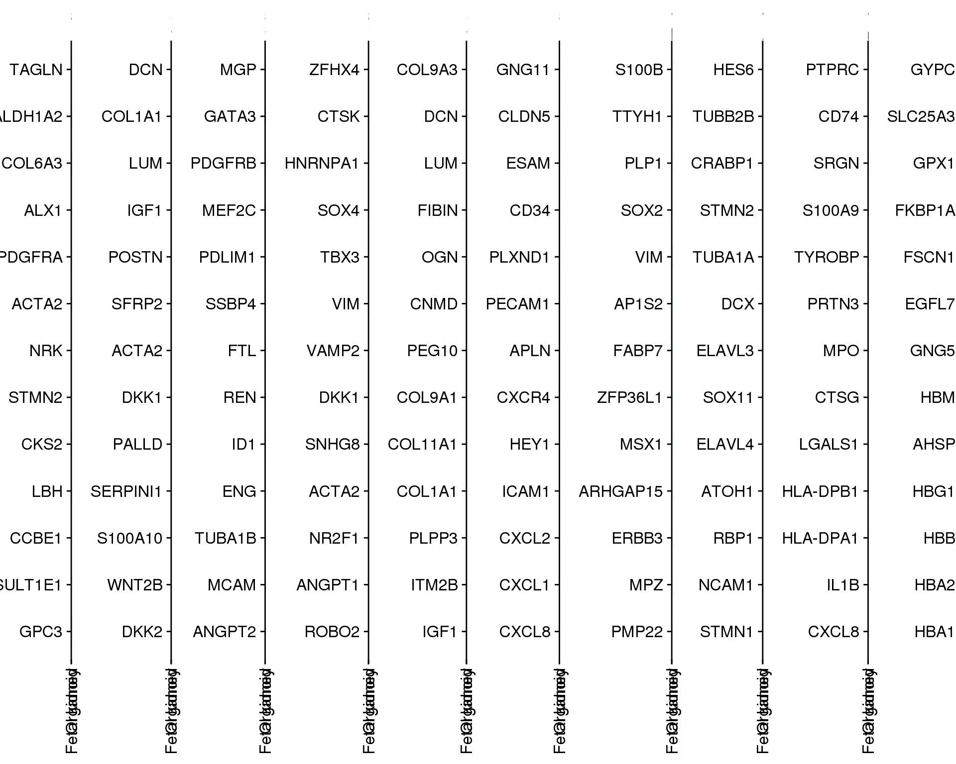
Figure 2 Panel
p1 <- plot_grid(f2A + theme(legend.position = "none"),
                f2B + theme(legend.position = "none"),
                nrow = 1, labels = c("A", "B"),
                label_size = 20)
p2 <- plot_grid(f2C, f2D, f2E,
                nrow = 1, rel_widths = c(1.1, 1, 0.5),
                labels = c("C", "D", "E"),
                label_size = 20)
panel <- plot_grid(p1, l2AB, p2, f2F, f2G, ncol = 1,
                   labels = c("", "", "", "F", "G"),
                   rel_heights = c(1, 0.22, 0.7, 0.4, 0.9),
                   label_size = 20)

ggsave(here("output", DOCNAME, "figure2_panel.png"), panel,
       height = 20, width = 16)
ggsave(here("output", DOCNAME, "figure2_panel.pdf"), panel,
       height = 20, width = 16)

panel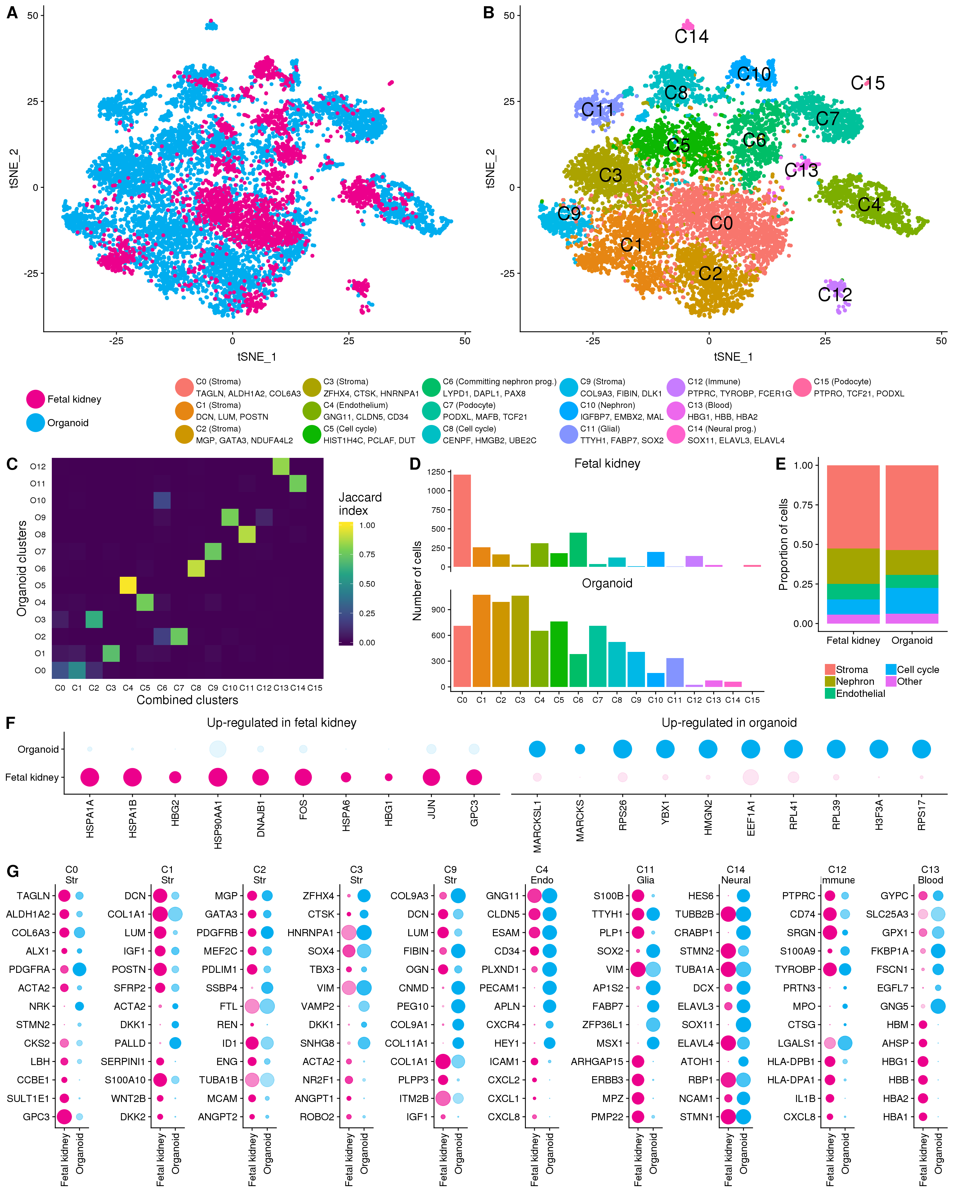
Figure 3
Figure 3A
plot.data <- comb.neph %>%
    GetDimReduction("tsne",  slot = "cell.embeddings") %>%
    data.frame() %>%
    rownames_to_column("Cell") %>%
    mutate(Group = comb.neph@meta.data$Group) %>%
    mutate(Group = if_else(Group == "Lindstrom", "Fetal kidney", Group))

f3A <- ggplot(plot.data, aes(x = tSNE_1, y = tSNE_2, colour = Group)) +
    geom_point(size = 3) +
    scale_color_manual(values = c("#EC008C", "#00ADEF")) +
    guides(colour = guide_legend(ncol = 4, override.aes = list(size = 12),
                                 label.theme = element_text(size = 12))) +
    theme_cowplot() +
    theme(legend.position = "bottom",
          legend.title = element_blank(),
          legend.justification = "center")

ggsave(here("output", DOCNAME, "figure3A.png"), f3A,
       height = 8, width = 10)
ggsave(here("output", DOCNAME, "figure3A.pdf"), f3A,
       height = 8, width = 10)

f3A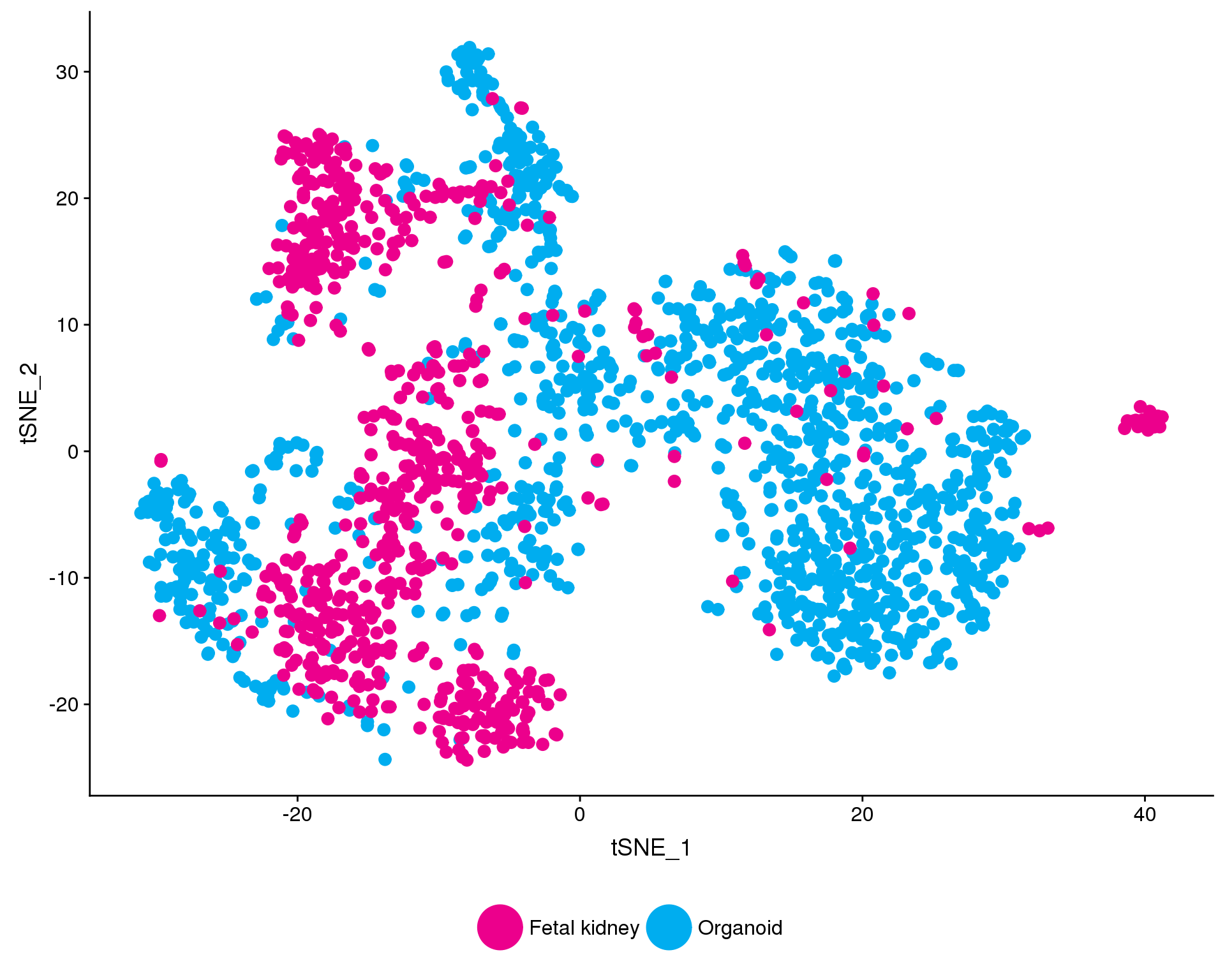
Expand here to see past versions of fig-3A-1.png:
| Version | Author | Date |
|---|---|---|
| a1f9f38 | Luke Zappia | 2018-11-23 |
Figure 3B
plot.data <- comb.neph %>%
    GetDimReduction("tsne",  slot = "cell.embeddings") %>%
    data.frame() %>%
    rownames_to_column("Cell") %>%
    mutate(Cluster = comb.neph@ident)

lab.data <- plot.data %>%
    group_by(Cluster) %>%
    summarise(tSNE_1 = mean(tSNE_1),
              tSNE_2 = mean(tSNE_2)) %>%
    mutate(Label = paste0("CN", Cluster))

clust.labs <- c(
    "CN0 (Podocyte)\nTCF21, PODXL, SYNPO",
    "CN1 (Differentiating nephron prog.)\nLYPD1, PAX8, DAPL1",
    "CN2 (Nephron progenitor)\nCRABP2, SIX1, TMEM100, CITED1",
    "CN3 (Podocyte precursor)\nCTGF, OLFM3, MAFB",
    "CN4 (Distal)\nWFDC2, EMX2, MAL, GATA3",
    "CN5 (Proximal)\nIGFBP7, MPC2, FXYD2, CDH6",
    "CN6 (Stroma)\nfetal kidney only",
    "CN7 (Podocyte)\nfetal kidney only"
)

f3B <- ggplot(plot.data, aes(x = tSNE_1, y = tSNE_2, colour = Cluster)) +
    geom_point(size = 3) +
    geom_text(data = lab.data, aes(label = Label), colour = "black", size = 8) +
    #scale_color_brewer(palette = "Set1", labels = clust.labs) +
    scale_colour_discrete(labels = clust.labs) +
    guides(colour = guide_legend(ncol = 4, override.aes = list(size = 12),
                                 label.theme = element_text(size = 12))) +
    theme_cowplot() +
    theme(legend.position = "bottom",
          legend.title = element_blank(),
          legend.justification = "center")

ggsave(here("output", DOCNAME, "figure3B.png"), f3B,
       height = 8, width = 10)
ggsave(here("output", DOCNAME, "figure3B.pdf"), f3B,
       height = 8, width = 10)

f3B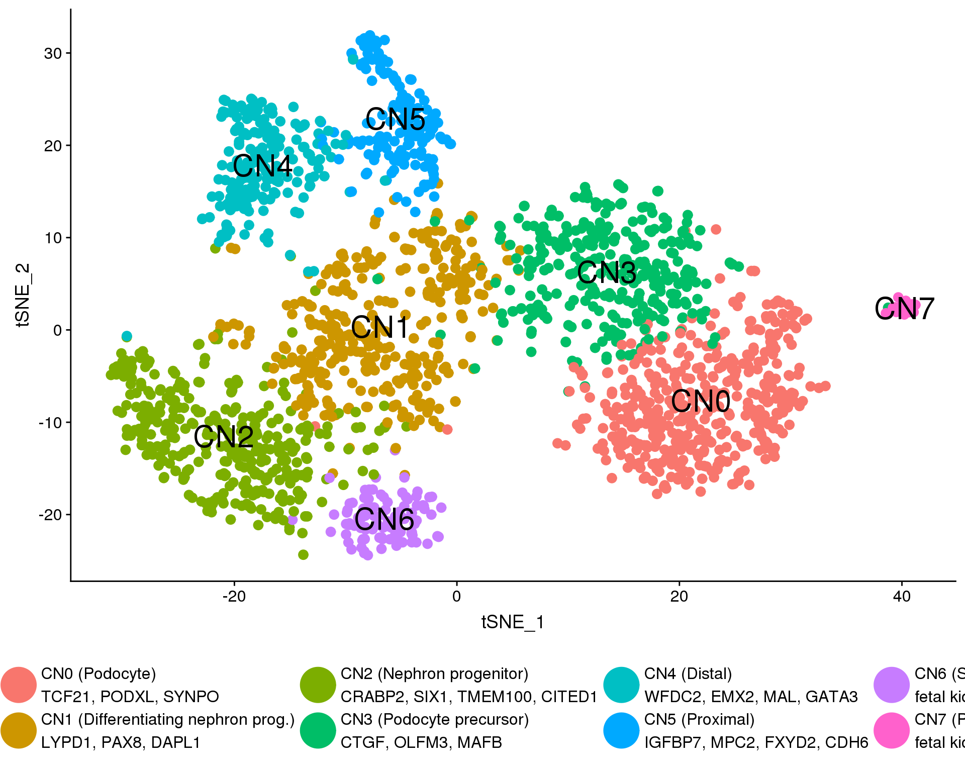
Expand here to see past versions of fig-3B-1.png:
| Version | Author | Date |
|---|---|---|
| a1f9f38 | Luke Zappia | 2018-11-23 |
Figure 3AB legend
l3A <- get_legend(f3A)
l3B <- get_legend(f3B)

l3AB <- plot_grid(l3A, l3B, nrow = 1, rel_widths = c(0.3, 1))

l3AB
Expand here to see past versions of fig-3AB-legend-1.png:
| Version | Author | Date |
|---|---|---|
| a1f9f38 | Luke Zappia | 2018-11-23 |
Figure 3C
f3C <- summariseClusts(clusts, CombNephron, OrgsNephron) %>%
    replace_na(list(Jaccard = 0)) %>%
    ggplot(aes(x = CombNephron, y = OrgsNephron, fill = Jaccard)) +
    geom_tile() +
    scale_fill_viridis_c(limits = c(0, 1), name = "Jaccard\nindex") +
    scale_x_discrete(labels = paste0("CN", 0:7)) +
    scale_y_discrete(labels = paste0("ON", 0:4)) +
    coord_equal() +
    xlab("Combined nephron clusters") +
    ylab("Organoid nephron clusters") +
    theme_minimal() +
    theme(axis.text = element_text(size = 10, colour = "black"),
          axis.ticks = element_blank(),
          axis.title = element_text(size = 16),
          legend.key.height = unit(30, "pt"),
          legend.title = element_text(size = 12),
          legend.text = element_text(size = 10),
          panel.grid = element_blank())

ggsave(here("output", DOCNAME, "figure3C.png"), f3C,
       height = 8, width = 10)
ggsave(here("output", DOCNAME, "figure3C.pdf"), f3C,
       height = 8, width = 10)

f3C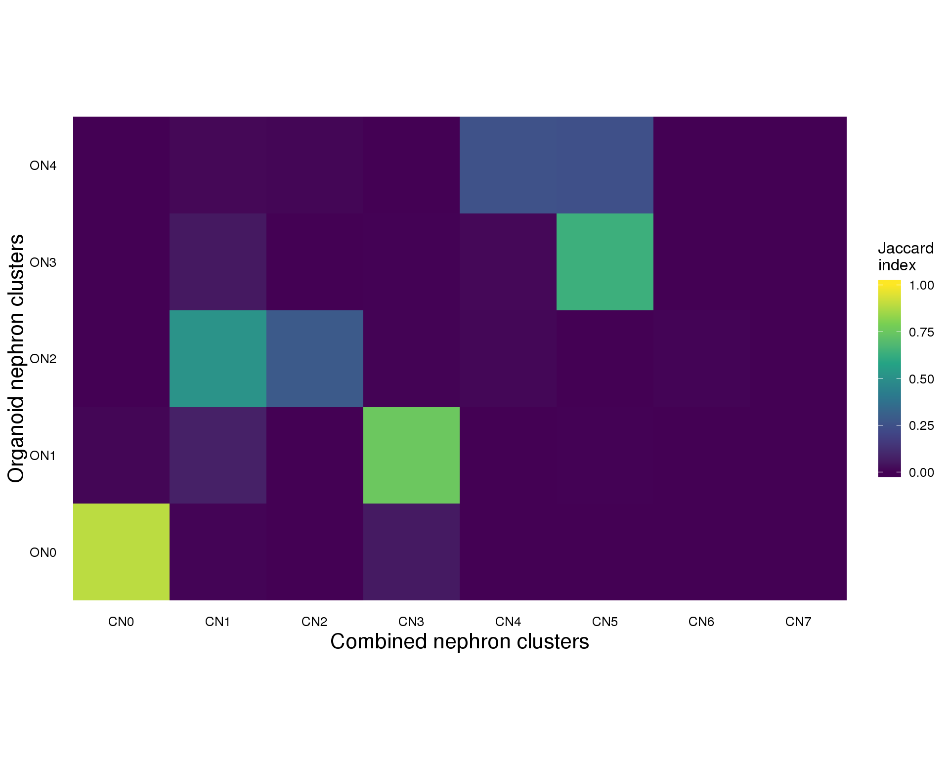
Figure 3D
plot.data <- comb.neph@meta.data %>%
    select(NephCluster, Group) %>%
    mutate(NephCluster = paste0("CN", NephCluster)) %>%
    mutate(Group = if_else(Group == "Lindstrom", "Fetal kidney", Group))

f3D <- ggplot(plot.data, aes(x = NephCluster, fill = NephCluster)) +
    geom_bar() +
    #scale_fill_brewer(palette = "Set1") +
    labs(y = "Number of cells") +
    facet_wrap(~ Group, ncol = 1, scales = "free_y") +
    theme_cowplot() +
    theme(legend.position = "none",
          axis.title.x = element_blank(),
          strip.text = element_text(size = 15,
                                    margin = margin(0, 0, 2, 0, "pt")),
          strip.background = element_blank(),
          strip.placement = "outside")

ggsave(here("output", DOCNAME, "figure3D.png"), f3D,
       height = 8, width = 10)
ggsave(here("output", DOCNAME, "figure3D.pdf"), f3D,
       height = 8, width = 10)

f3D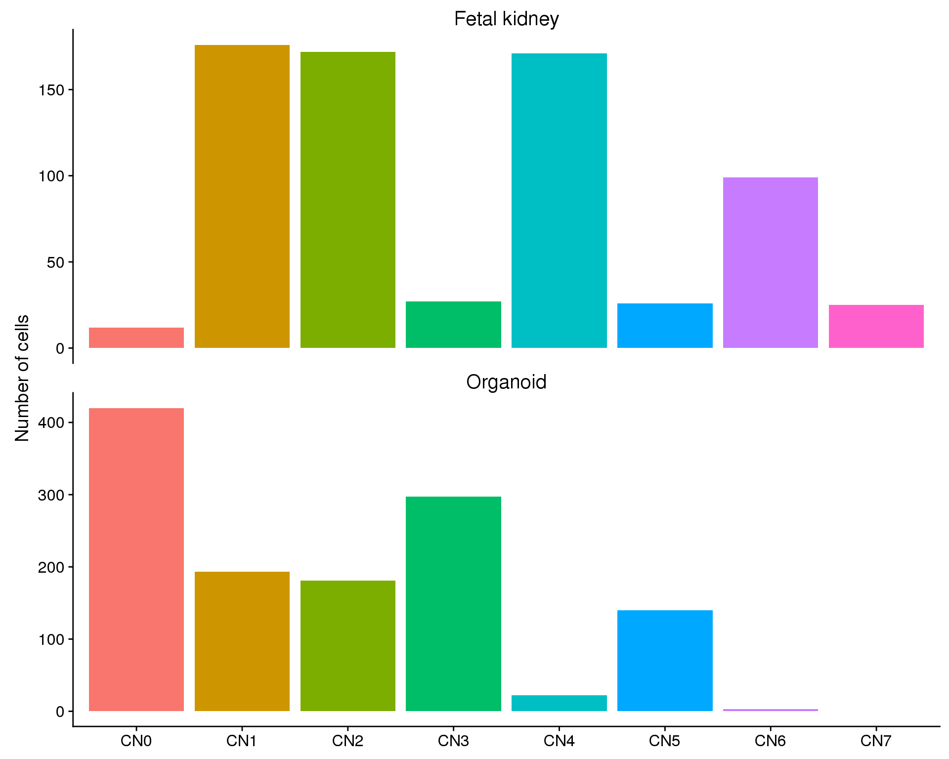
Expand here to see past versions of fig-3D-1.png:
| Version | Author | Date |
|---|---|---|
| a1f9f38 | Luke Zappia | 2018-11-23 |
Figure 3E
genes <- c( "TCF21",   "ROBO2",  "NPHS2", "NPHS1",   "SYNPO",
            "LYPD1",    "PAX8",  "DAPL1",  "CDH6",    "PAX2",   "HEY1",
             "SIX1", "TMEM100", "CITED1", "MEOX1",    "EYA1", "CRABP2",
             "CTGF",   "OLFM3",   "MAFB", "PODXL",   "VAMP8",
            "WFDC2",    "EMX2",    "MAL", "MECOM", "TMEM52B",
           "IGFBP7",   "FXYD2",    "CLU",  "MPC2",
           "COL1A1",  "COL3A1",  "SNAI2", "POSTN",  "LGALS1",
            "PTPRO",   "TPPP3",  "CLIC5", "ENPEP",     "GSN", "TSPAN2")

gene.groups <- rev(c(rep("Podocyte", 5),
                     rep("Differentiating\nnephron progenitor", 6),
                     rep("Nephron\nprogenitor", 6),
                     rep("Podocyte\nprecursor", 5),
                     rep("Distal", 5),
                     rep("Proximal", 4),
                     rep("Stroma", 5),
                     rep("hFK\nPodocyte", 6))) %>%
    fct_relevel("Podocyte", "Differentiating\nnephron progenitor",
                "Nephron\nprogenitor", "Podocyte\nprecursor", "Distal",
                "Proximal", "Stroma", "hFK\nPodocyte")

clust.labs <- c(
    "hFK CN0", "Org CN0",
    "hFK CN1", "Org CN1",
    "hFK CN2", "Org CN2",
    "hFK CN3", "Org CN3",
    "hFK CN4", "Org CN4",
    "hFK CN5", "Org CN5",
    "hFK CN6", "Org CN6",
    "hFK CN7", "Org CN7"
)

f3E <- SplitDotPlotGG(comb.neph, "Group", genes, gene.groups,
                      cols.use = c("#EC008C", "#00ADEF"), dot.scale = 5,
                      do.return = TRUE) +
    scale_y_discrete(labels = clust.labs) +
    theme(axis.text.x = element_text(angle = 90, vjust = 0.5, hjust = 1),
          strip.text.x = element_text(margin = margin(0, 0, 2, 0, "pt")))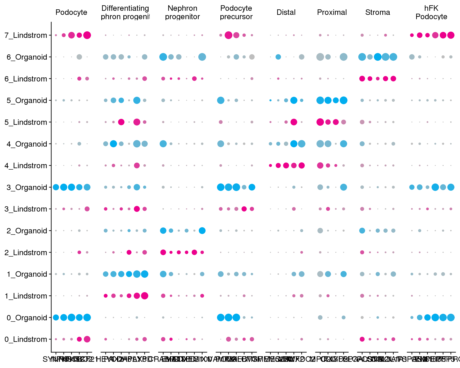
Expand here to see past versions of fig-3E-1.png:
| Version | Author | Date |
|---|---|---|
| 1b1ce1c | Luke Zappia | 2018-11-23 |
| a1f9f38 | Luke Zappia | 2018-11-23 |
for (y in seq(2.5, 14.5, 2)) {
    f3E <- f3E + geom_hline(yintercept = y, size = 0.2, colour = "grey70")
}

ggsave(here("output", DOCNAME, "figure3E.png"), f3E,
       height = 4, width = 20)
ggsave(here("output", DOCNAME, "figure3E.pdf"), f3E,
       height = 8, width = 10)

f3E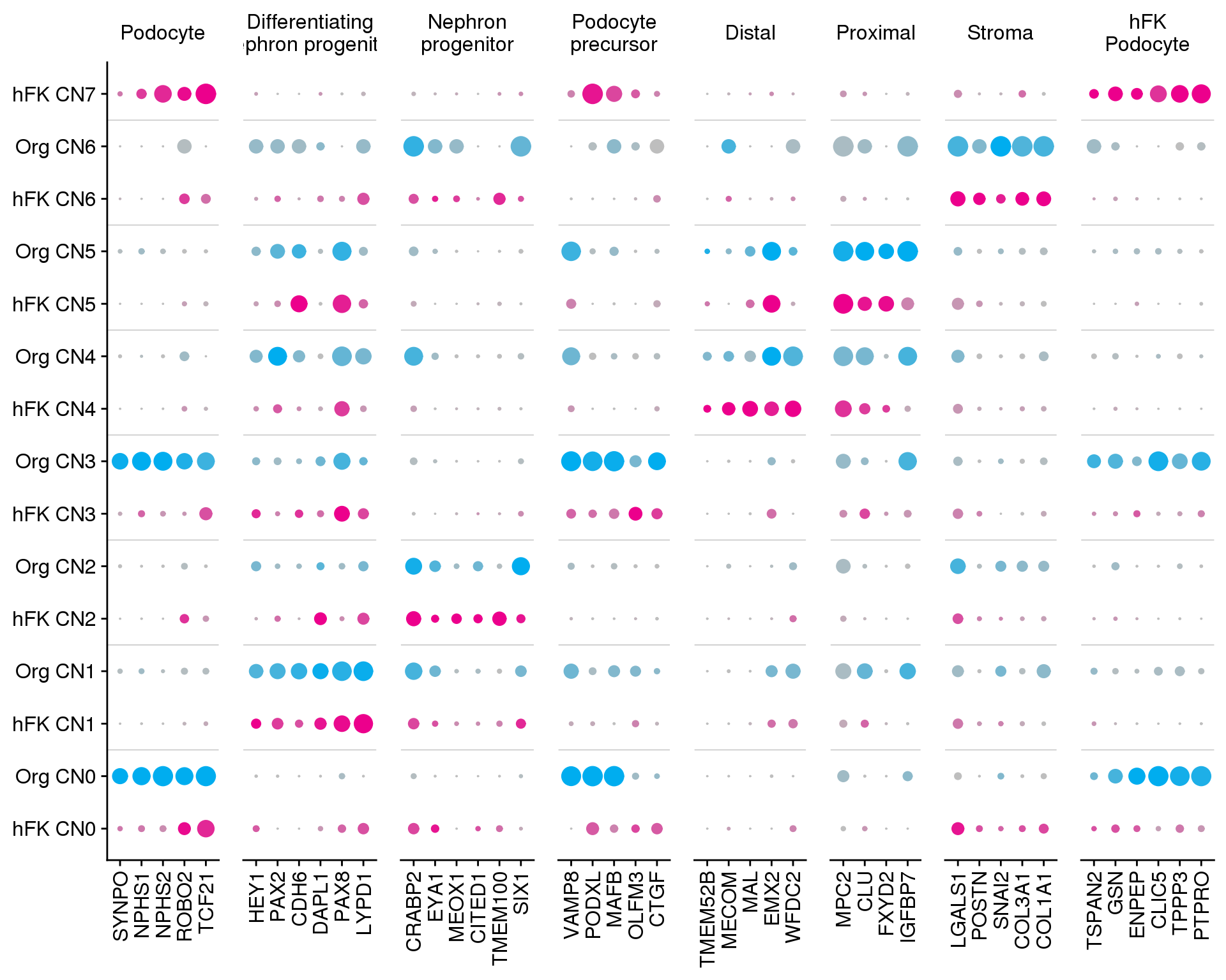
Figure 3F
genes.list <- list(
    c("LYPD1", "PDGFC", "ITGA8", "TUBA1A", "PTPRO", "WT1", "ANXA1", "VAMP8"),
    c("CCND1", "CXCR4", "TUBA1B", "STMN1", "ATOX1", "BNIP3", "GNAS", "FTL"),
    c("TMEM100", "MEOX1", "ROBO2", "DAPL1", "MYOD1", "MYOG", "PITX2", "TPM2"),
    c("HNRNPR", "CXCL1", "OLFM3", "CCND1_1", "PTPRO_1", "WT1_1", "VEGFA",
      "SYNPO"),
    c("PAPPA2", "LIMCH1", "MAL", "PTGR1", "CITED2", "FTL_1", "BNIP3_1",
      "LHX1"),
    c("VCAN", "PSMA2", "CA2", "CCND1_2", "VAMP8_1", "BNIP3_2", "LHX1_1",
      "HNF1B"),
    c("COL1A1", "COL3A1", "SERPINH1", "POSTN", "MEG3", "COL1A2", "CYR61",
      "MEIS2"),
    c("TNNI1", "TNNT2", "MRGPRF", "MYL9", "COL4A4", "TUBB2A", "HMGCS1", "MSMO1")
)

clust.labs <- c("CN0\nPodocyte", "CN1\nDiff. NP", "CN2\nNP", "CN3\nPod. Pre.",
                "CN4\nDistal", "CN5\nProximal", "CN6\nStroma", "CN7\nPodocyte")

plot.data <- lapply(seq_along(genes.list), function(idx) {
    genes.raw <- genes.list[[idx]]
    genes <- str_remove(genes.raw, "_[0-9]")
    names(genes.raw) <- genes
    comb.neph %>%
        FetchData(vars.all = genes) %>%
        as_data_frame() %>%
        rownames_to_column("Cell") %>%
        mutate(Cluster = as.numeric(as.character(comb.neph@ident)),
               Group = comb.neph@meta.data$Group) %>%
        gather(key = "Gene", value = "Expr", -Cell, -Cluster, -Group) %>%
        group_by(Cluster, Gene, Group) %>%
        summarize(AvgExpr = mean(expm1(Expr)),
                  PctExpr = Seurat:::PercentAbove(Expr, threshold = 0) * 100) %>%
        group_by(Gene) %>%
        mutate(AvgExprScale = scale(AvgExpr)) %>%
        mutate(AvgExprScale = Seurat::MinMax(AvgExprScale,
                                             max = 2.5, min = -2.5)) %>%
        filter(Cluster == idx - 1)  %>%
        ungroup() %>%
        mutate(Gene = genes.raw[Gene])
})

plot.data <- plot.data %>%
    bind_rows() %>%
    mutate(Cluster = factor(Cluster, labels = clust.labs)) %>%
    mutate(Gene = factor(Gene, levels = unlist(genes.list)))

f3F <- ggplot(plot.data,
              aes(x = Group, y = Gene, size = PctExpr,
                  colour = Group, alpha = AvgExprScale)) +
    geom_point() +
    scale_radius(range = c(0, 10)) +
    scale_alpha(range = c(0.1, 1)) +
    scale_colour_manual(values = c("#EC008C", "#00ADEF")) +
    scale_x_discrete(labels = c("Fetal kidney", "Organoid")) +
    scale_y_discrete(labels = str_remove(unlist(genes.list), "_[0-9]"),
                     breaks = unlist(genes.list)) +
    facet_wrap(~ Cluster, scales = "free", nrow = 1) +
    theme(axis.title.x = element_blank(),
          axis.title.y = element_blank(),
          axis.text.x = element_text(angle = 90, vjust = 0.5, hjust = 1),
          panel.spacing = unit(x = 1, units = "lines"),
          strip.background = element_blank(),
          strip.placement = "outside",
          legend.position = "none")

ggsave(here("output", DOCNAME, "figure3F.png"), f3F,
       height = 8, width = 10)
ggsave(here("output", DOCNAME, "figure3F.pdf"), f3F,
       height = 8, width = 10)

f3F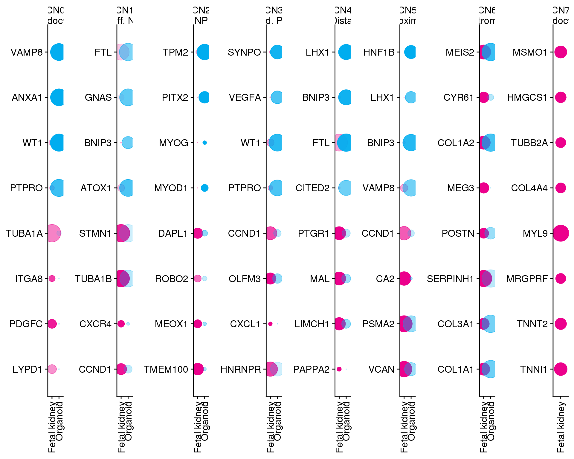
Figure 3 Panel
p1 <- plot_grid(f3A + theme(legend.position = "none"),
                f3B + theme(legend.position = "none"),
                nrow = 1, labels = c("A", "B"),
                label_size = 20)
p2 <- plot_grid(f3C, f3D,
                nrow = 1, labels = c("C", "D"),
                label_size = 20)
p3 <- plot_grid(p1,
                l3AB,
                p2,
                ncol = 1, rel_heights = c(1, 0.2, 0.6))
panel <- plot_grid(p3, f3E, f3F, ncol = 1, labels = c("", "E", "F"),
                   rel_heights = c(1, 0.4, 0.4),
                   label_size = 20)

ggsave(here("output", DOCNAME, "figure3_panel.png"), panel,
       height = 20, width = 16)
ggsave(here("output", DOCNAME, "figure3_panel.pdf"), panel,
       height = 20, width = 16)

panel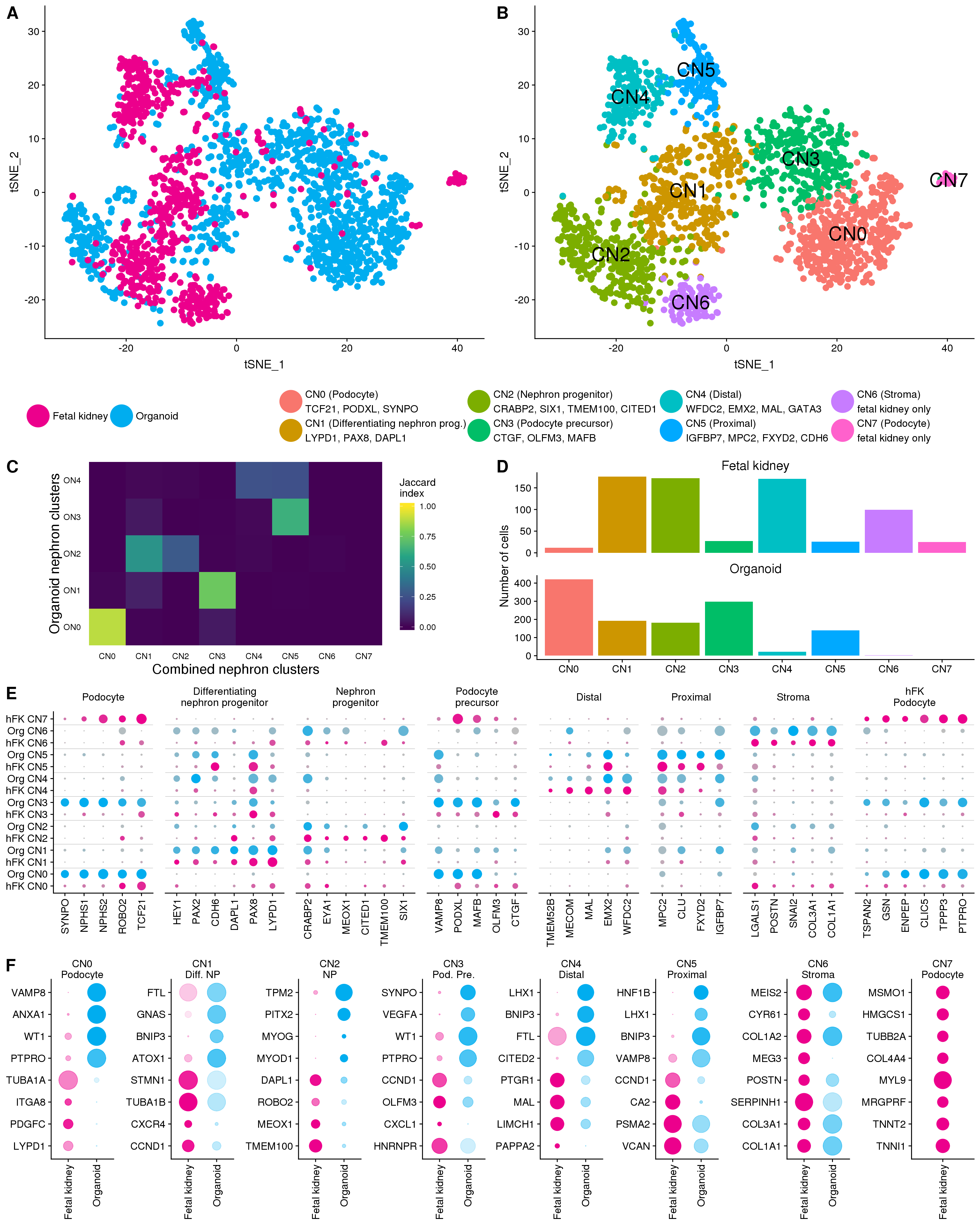
Summary
Output files
This table describes the output files produced by this document. Right click and Save Link As… to download the results.
kable(data.frame(
    File = c(
        glue("[figure2A.png]({getDownloadURL('figure2A.png', DOCNAME)})"),
        glue("[figure2A.pdf]({getDownloadURL('figure2A.pdf', DOCNAME)})"),
        glue("[figure2B.png]({getDownloadURL('figure2B.png', DOCNAME)})"),
        glue("[figure2B.pdf]({getDownloadURL('figure2B.pdf', DOCNAME)})"),
        glue("[figure2C.png]({getDownloadURL('figure2C.png', DOCNAME)})"),
        glue("[figure2C.pdf]({getDownloadURL('figure2C.pdf', DOCNAME)})"),
        glue("[figure2D.png]({getDownloadURL('figure2D.png', DOCNAME)})"),
        glue("[figure2D.pdf]({getDownloadURL('figure2D.pdf', DOCNAME)})"),
        glue("[figure2E.png]({getDownloadURL('figure2E.png', DOCNAME)})"),
        glue("[figure2E.pdf]({getDownloadURL('figure2E.pdf', DOCNAME)})"),
        glue("[figure2F.png]({getDownloadURL('figure2F.png', DOCNAME)})"),
        glue("[figure2F.pdf]({getDownloadURL('figure2F.pdf', DOCNAME)})"),
        glue("[figure2G.png]({getDownloadURL('figure2G.png', DOCNAME)})"),
        glue("[figure2G.pdf]({getDownloadURL('figure2G.pdf', DOCNAME)})"),
        glue("[figure2_panel.png]",
             "({getDownloadURL('figure2_panel.png', DOCNAME)})"),
        glue("[figure2_panel.pdf]",
             "({getDownloadURL('figure2_panel.pdf', DOCNAME)})"),
        glue("[figure3A.png]({getDownloadURL('figure3A.png', DOCNAME)})"),
        glue("[figure3A.pdf]({getDownloadURL('figure3A.pdf', DOCNAME)})"),
        glue("[figure3B.png]({getDownloadURL('figure3B.png', DOCNAME)})"),
        glue("[figure3B.pdf]({getDownloadURL('figure3B.pdf', DOCNAME)})"),
        glue("[figure3C.png]({getDownloadURL('figure3C.png', DOCNAME)})"),
        glue("[figure3C.pdf]({getDownloadURL('figure3C.pdf', DOCNAME)})"),
        glue("[figure3D.png]({getDownloadURL('figure3D.png', DOCNAME)})"),
        glue("[figure3D.pdf]({getDownloadURL('figure3D.pdf', DOCNAME)})"),
        glue("[figure3E.png]({getDownloadURL('figure3E.png', DOCNAME)})"),
        glue("[figure3E.pdf]({getDownloadURL('figure3E.pdf', DOCNAME)})"),
        glue("[figure3F.png]({getDownloadURL('figure3F.png', DOCNAME)})"),
        glue("[figure3F.pdf]({getDownloadURL('figure3F.pdf', DOCNAME)})"),
        glue("[figure3_panel.png]",
             "({getDownloadURL('figure3_panel.png', DOCNAME)})"),
        glue("[figure3_panel.pdf]",
             "({getDownloadURL('figure3_panel.pdf', DOCNAME)})")
    ),
    Description = c(
        "Figure 2A in PNG format",
        "Figure 2A in PDF format",
        "Figure 2B in PNG format",
        "Figure 2B in PDF format",
        "Figure 2C in PNG format",
        "Figure 2C in PDF format",
        "Figure 2D in PNG format",
        "Figure 2D in PDF format",
        "Figure 2E in PNG format",
        "Figure 2E in PDF format",
        "Figure 2F in PNG format",
        "Figure 2F in PDF format",
        "Figure 2G in PNG format",
        "Figure 2G in PDF format",
        "Figure 2 panel in PNG format",
        "Figure 2 panel in PDF format",
        "Figure 3A in PNG format",
        "Figure 3A in PDF format",
        "Figure 3B in PNG format",
        "Figure 3B in PDF format",
        "Figure 3C in PNG format",
        "Figure 3C in PDF format",
        "Figure 3D in PNG format",
        "Figure 3D in PDF format",
        "Figure 3E in PNG format",
        "Figure 3E in PDF format",
        "Figure 3F in PNG format",
        "Figure 3F in PDF format",
        "Figure 3 panel in PNG format",
        "Figure 3 panel in PDF format"
    )
))| File | Description |
|---|---|
| figure2A.png | Figure 2A in PNG format |
| figure2A.pdf | Figure 2A in PDF format |
| figure2B.png | Figure 2B in PNG format |
| figure2B.pdf | Figure 2B in PDF format |
| figure2C.png | Figure 2C in PNG format |
| figure2C.pdf | Figure 2C in PDF format |
| figure2D.png | Figure 2D in PNG format |
| figure2D.pdf | Figure 2D in PDF format |
| figure2E.png | Figure 2E in PNG format |
| figure2E.pdf | Figure 2E in PDF format |
| figure2F.png | Figure 2F in PNG format |
| figure2F.pdf | Figure 2F in PDF format |
| figure2G.png | Figure 2G in PNG format |
| figure2G.pdf | Figure 2G in PDF format |
| figure2_panel.png | Figure 2 panel in PNG format |
| figure2_panel.pdf | Figure 2 panel in PDF format |
| figure3A.png | Figure 3A in PNG format |
| figure3A.pdf | Figure 3A in PDF format |
| figure3B.png | Figure 3B in PNG format |
| figure3B.pdf | Figure 3B in PDF format |
| figure3C.png | Figure 3C in PNG format |
| figure3C.pdf | Figure 3C in PDF format |
| figure3D.png | Figure 3D in PNG format |
| figure3D.pdf | Figure 3D in PDF format |
| figure3E.png | Figure 3E in PNG format |
| figure3E.pdf | Figure 3E in PDF format |
| figure3F.png | Figure 3F in PNG format |
| figure3F.pdf | Figure 3F in PDF format |
| figure3_panel.png | Figure 3 panel in PNG format |
| figure3_panel.pdf | Figure 3 panel in PDF format |
Session information
devtools::session_info() setting value
version R version 3.5.0 (2018-04-23)
system x86_64, linux-gnu
ui X11
language (EN)
collate en_US.UTF-8
tz Australia/Melbourne
date 2019-01-07
package * version date source
abind 1.4-5 2016-07-21 cran (@1.4-5)
acepack 1.4.1 2016-10-29 cran (@1.4.1)
ape 5.1 2018-04-04 cran (@5.1)
assertthat 0.2.0 2017-04-11 CRAN (R 3.5.0)
backports 1.1.2 2017-12-13 CRAN (R 3.5.0)
base * 3.5.0 2018-06-18 local
base64enc 0.1-3 2015-07-28 CRAN (R 3.5.0)
bibtex 0.4.2 2017-06-30 cran (@0.4.2)
bindr 0.1.1 2018-03-13 cran (@0.1.1)
bindrcpp 0.2.2 2018-03-29 cran (@0.2.2)
Biobase * 2.40.0 2018-07-30 Bioconductor
BiocGenerics * 0.26.0 2018-07-30 Bioconductor
bitops 1.0-6 2013-08-17 cran (@1.0-6)
broom 0.5.0 2018-07-17 cran (@0.5.0)
caret 6.0-80 2018-05-26 cran (@6.0-80)
caTools 1.17.1.1 2018-07-20 cran (@1.17.1.)
cellranger 1.1.0 2016-07-27 CRAN (R 3.5.0)
checkmate 1.8.5 2017-10-24 cran (@1.8.5)
class 7.3-14 2015-08-30 CRAN (R 3.5.0)
cli 1.0.0 2017-11-05 CRAN (R 3.5.0)
cluster 2.0.7-1 2018-04-13 CRAN (R 3.5.0)
clustree * 0.2.2.9000 2018-08-01 Github (lazappi/clustree@66a865b)
codetools 0.2-15 2016-10-05 CRAN (R 3.5.0)
colorspace 1.3-2 2016-12-14 cran (@1.3-2)
combinat 0.0-8 2012-10-29 CRAN (R 3.5.0)
compiler 3.5.0 2018-06-18 local
cowplot * 0.9.3 2018-07-15 cran (@0.9.3)
crayon 1.3.4 2017-09-16 CRAN (R 3.5.0)
CVST 0.2-2 2018-05-26 cran (@0.2-2)
data.table 1.11.4 2018-05-27 cran (@1.11.4)
datasets * 3.5.0 2018-06-18 local
ddalpha 1.3.4 2018-06-23 cran (@1.3.4)
DDRTree * 0.1.5 2017-04-30 CRAN (R 3.5.0)
densityClust 0.3 2017-10-24 CRAN (R 3.5.0)
DEoptimR 1.0-8 2016-11-19 cran (@1.0-8)
devtools 1.13.6 2018-06-27 CRAN (R 3.5.0)
diffusionMap 1.1-0.1 2018-07-21 cran (@1.1-0.1)
digest 0.6.15 2018-01-28 CRAN (R 3.5.0)
dimRed 0.1.0 2017-05-04 cran (@0.1.0)
diptest 0.75-7 2016-12-05 cran (@0.75-7)
docopt 0.6 2018-08-03 CRAN (R 3.5.0)
doSNOW 1.0.16 2017-12-13 cran (@1.0.16)
dplyr * 0.7.6 2018-06-29 cran (@0.7.6)
DRR 0.0.3 2018-01-06 cran (@0.0.3)
dtw 1.20-1 2018-05-18 cran (@1.20-1)
evaluate 0.10.1 2017-06-24 CRAN (R 3.5.0)
fastICA 1.2-1 2017-06-12 CRAN (R 3.5.0)
fitdistrplus 1.0-9 2017-03-24 cran (@1.0-9)
flexmix 2.3-14 2017-04-28 cran (@2.3-14)
FNN 1.1 2013-07-31 cran (@1.1)
forcats * 0.3.0 2018-02-19 CRAN (R 3.5.0)
foreach 1.4.4 2017-12-12 cran (@1.4.4)
foreign 0.8-71 2018-07-20 CRAN (R 3.5.0)
Formula 1.2-3 2018-05-03 cran (@1.2-3)
fpc 2.1-11.1 2018-07-20 cran (@2.1-11.)
gbRd 0.4-11 2012-10-01 cran (@0.4-11)
gdata 2.18.0 2017-06-06 cran (@2.18.0)
geometry 0.3-6 2015-09-09 cran (@0.3-6)
ggforce 0.1.3 2018-07-07 CRAN (R 3.5.0)
ggplot2 * 3.0.0 2018-07-03 cran (@3.0.0)
ggraph * 1.0.2 2018-07-07 CRAN (R 3.5.0)
ggrepel 0.8.0 2018-05-09 CRAN (R 3.5.0)
ggridges 0.5.0 2018-04-05 cran (@0.5.0)
git2r 0.21.0 2018-01-04 CRAN (R 3.5.0)
glue * 1.3.0 2018-07-17 cran (@1.3.0)
gower 0.1.2 2017-02-23 cran (@0.1.2)
gplots 3.0.1 2016-03-30 cran (@3.0.1)
graphics * 3.5.0 2018-06-18 local
grDevices * 3.5.0 2018-06-18 local
grid 3.5.0 2018-06-18 local
gridExtra 2.3 2017-09-09 cran (@2.3)
gtable 0.2.0 2016-02-26 cran (@0.2.0)
gtools 3.8.1 2018-06-26 cran (@3.8.1)
haven 1.1.2 2018-06-27 CRAN (R 3.5.0)
here * 0.1 2017-05-28 CRAN (R 3.5.0)
Hmisc 4.1-1 2018-01-03 cran (@4.1-1)
hms 0.4.2 2018-03-10 CRAN (R 3.5.0)
HSMMSingleCell 0.114.0 2018-08-28 Bioconductor
htmlTable 1.12 2018-05-26 cran (@1.12)
htmltools 0.3.6 2017-04-28 CRAN (R 3.5.0)
htmlwidgets 1.2 2018-04-19 cran (@1.2)
httr 1.3.1 2017-08-20 CRAN (R 3.5.0)
ica 1.0-2 2018-05-24 cran (@1.0-2)
igraph 1.2.2 2018-07-27 cran (@1.2.2)
ipred 0.9-6 2017-03-01 cran (@0.9-6)
irlba * 2.3.2 2018-01-11 cran (@2.3.2)
iterators 1.0.10 2018-07-13 cran (@1.0.10)
jsonlite 1.5 2017-06-01 CRAN (R 3.5.0)
kernlab 0.9-26 2018-04-30 cran (@0.9-26)
KernSmooth 2.23-15 2015-06-29 CRAN (R 3.5.0)
knitr * 1.20 2018-02-20 CRAN (R 3.5.0)
lars 1.2 2013-04-24 cran (@1.2)
lattice 0.20-35 2017-03-25 CRAN (R 3.5.0)
latticeExtra 0.6-28 2016-02-09 cran (@0.6-28)
lava 1.6.2 2018-07-02 cran (@1.6.2)
lazyeval 0.2.1 2017-10-29 cran (@0.2.1)
limma 3.36.2 2018-06-21 Bioconductor
lmtest 0.9-36 2018-04-04 cran (@0.9-36)
lubridate 1.7.4 2018-04-11 cran (@1.7.4)
magic 1.5-8 2018-01-26 cran (@1.5-8)
magrittr 1.5 2014-11-22 CRAN (R 3.5.0)
MASS 7.3-50 2018-04-30 CRAN (R 3.5.0)
Matrix * 1.2-14 2018-04-09 CRAN (R 3.5.0)
matrixStats 0.54.0 2018-07-23 CRAN (R 3.5.0)
mclust 5.4.1 2018-06-27 cran (@5.4.1)
memoise 1.1.0 2017-04-21 CRAN (R 3.5.0)
metap 1.0 2018-07-25 cran (@1.0)
methods * 3.5.0 2018-06-18 local
mixtools 1.1.0 2017-03-10 cran (@1.1.0)
ModelMetrics 1.1.0 2016-08-26 cran (@1.1.0)
modelr 0.1.2 2018-05-11 CRAN (R 3.5.0)
modeltools 0.2-22 2018-07-16 cran (@0.2-22)
monocle * 2.8.0 2018-08-28 Bioconductor
munsell 0.5.0 2018-06-12 cran (@0.5.0)
mvtnorm 1.0-8 2018-05-31 cran (@1.0-8)
nlme 3.1-137 2018-04-07 CRAN (R 3.5.0)
nnet 7.3-12 2016-02-02 CRAN (R 3.5.0)
parallel * 3.5.0 2018-06-18 local
pbapply 1.3-4 2018-01-10 cran (@1.3-4)
pheatmap 1.0.10 2018-05-19 CRAN (R 3.5.0)
pillar 1.3.0 2018-07-14 cran (@1.3.0)
pkgconfig 2.0.1 2017-03-21 cran (@2.0.1)
pls 2.6-0 2016-12-18 cran (@2.6-0)
plyr 1.8.4 2016-06-08 cran (@1.8.4)
png 0.1-7 2013-12-03 cran (@0.1-7)
prabclus 2.2-6 2015-01-14 cran (@2.2-6)
prodlim 2018.04.18 2018-04-18 cran (@2018.04)
proxy 0.4-22 2018-04-08 cran (@0.4-22)
purrr * 0.2.5 2018-05-29 cran (@0.2.5)
qlcMatrix 0.9.7 2018-04-20 CRAN (R 3.5.0)
R.methodsS3 1.7.1 2016-02-16 CRAN (R 3.5.0)
R.oo 1.22.0 2018-04-22 CRAN (R 3.5.0)
R.utils 2.6.0 2017-11-05 CRAN (R 3.5.0)
R6 2.2.2 2017-06-17 CRAN (R 3.5.0)
ranger 0.10.1 2018-06-04 cran (@0.10.1)
RANN 2.6 2018-07-16 cran (@2.6)
RColorBrewer 1.1-2 2014-12-07 cran (@1.1-2)
Rcpp 0.12.18 2018-07-23 cran (@0.12.18)
RcppRoll 0.3.0 2018-06-05 cran (@0.3.0)
Rdpack 0.8-0 2018-05-24 cran (@0.8-0)
readr * 1.1.1 2017-05-16 CRAN (R 3.5.0)
readxl 1.1.0 2018-04-20 CRAN (R 3.5.0)
recipes 0.1.3 2018-06-16 cran (@0.1.3)
reshape2 1.4.3 2017-12-11 cran (@1.4.3)
reticulate 1.9 2018-07-06 cran (@1.9)
rlang 0.2.1 2018-05-30 CRAN (R 3.5.0)
rmarkdown 1.10.2 2018-07-30 Github (rstudio/rmarkdown@18207b9)
robustbase 0.93-2 2018-07-27 cran (@0.93-2)
ROCR 1.0-7 2015-03-26 cran (@1.0-7)
rpart 4.1-13 2018-02-23 CRAN (R 3.5.0)
rprojroot 1.3-2 2018-01-03 CRAN (R 3.5.0)
rstudioapi 0.7 2017-09-07 CRAN (R 3.5.0)
Rtsne 0.13 2017-04-14 cran (@0.13)
rvest 0.3.2 2016-06-17 CRAN (R 3.5.0)
scales 0.5.0 2017-08-24 cran (@0.5.0)
scatterplot3d 0.3-41 2018-03-14 cran (@0.3-41)
SDMTools 1.1-221 2014-08-05 cran (@1.1-221)
segmented 0.5-3.0 2017-11-30 cran (@0.5-3.0)
Seurat * 2.3.1 2018-05-05 url
sfsmisc 1.1-2 2018-03-05 cran (@1.1-2)
slam 0.1-43 2018-04-23 CRAN (R 3.5.0)
snow 0.4-2 2016-10-14 cran (@0.4-2)
sparsesvd 0.1-4 2018-02-15 CRAN (R 3.5.0)
splines * 3.5.0 2018-06-18 local
stats * 3.5.0 2018-06-18 local
stats4 * 3.5.0 2018-06-18 local
stringi 1.2.4 2018-07-20 cran (@1.2.4)
stringr * 1.3.1 2018-05-10 CRAN (R 3.5.0)
survival 2.42-6 2018-07-13 CRAN (R 3.5.0)
tclust 1.4-1 2018-05-24 cran (@1.4-1)
tibble * 1.4.2 2018-01-22 cran (@1.4.2)
tidyr * 0.8.1 2018-05-18 cran (@0.8.1)
tidyselect 0.2.4 2018-02-26 cran (@0.2.4)
tidyverse * 1.2.1 2017-11-14 CRAN (R 3.5.0)
timeDate 3043.102 2018-02-21 cran (@3043.10)
tools 3.5.0 2018-06-18 local
trimcluster 0.1-2.1 2018-07-20 cran (@0.1-2.1)
tsne 0.1-3 2016-07-15 cran (@0.1-3)
tweenr 0.1.5 2016-10-10 CRAN (R 3.5.0)
units 0.6-0 2018-06-09 CRAN (R 3.5.0)
utils * 3.5.0 2018-06-18 local
VGAM * 1.0-5 2018-02-07 cran (@1.0-5)
viridis 0.5.1 2018-03-29 cran (@0.5.1)
viridisLite 0.3.0 2018-02-01 cran (@0.3.0)
whisker 0.3-2 2013-04-28 CRAN (R 3.5.0)
withr 2.1.2 2018-03-15 CRAN (R 3.5.0)
workflowr 1.1.1 2018-07-06 CRAN (R 3.5.0)
xml2 1.2.0 2018-01-24 CRAN (R 3.5.0)
yaml 2.2.0 2018-07-25 cran (@2.2.0)
zoo 1.8-3 2018-07-16 cran (@1.8-3) This reproducible R Markdown analysis was created with workflowr 1.1.1