Crossover
Last updated: 2018-11-23
workflowr checks: (Click a bullet for more information)-
✔ R Markdown file: up-to-date
Great! Since the R Markdown file has been committed to the Git repository, you know the exact version of the code that produced these results.
-
✔ Environment: empty
Great job! The global environment was empty. Objects defined in the global environment can affect the analysis in your R Markdown file in unknown ways. For reproduciblity it’s best to always run the code in an empty environment.
-
✔ Seed:
set.seed(20180730)The command
set.seed(20180730)was run prior to running the code in the R Markdown file. Setting a seed ensures that any results that rely on randomness, e.g. subsampling or permutations, are reproducible. -
✔ Session information: recorded
Great job! Recording the operating system, R version, and package versions is critical for reproducibility.
-
Great! You are using Git for version control. Tracking code development and connecting the code version to the results is critical for reproducibility. The version displayed above was the version of the Git repository at the time these results were generated.✔ Repository version: 7d8a1dd
Note that you need to be careful to ensure that all relevant files for the analysis have been committed to Git prior to generating the results (you can usewflow_publishorwflow_git_commit). workflowr only checks the R Markdown file, but you know if there are other scripts or data files that it depends on. Below is the status of the Git repository when the results were generated:
Note that any generated files, e.g. HTML, png, CSS, etc., are not included in this status report because it is ok for generated content to have uncommitted changes.Ignored files: Ignored: .DS_Store Ignored: .Rhistory Ignored: .Rproj.user/ Ignored: analysis/cache.bak.20181031/ Ignored: analysis/cache.bak/ Ignored: analysis/cache.lind2.20181114/ Ignored: analysis/cache/ Ignored: data/Lindstrom2/ Ignored: data/processed.bak.20181031/ Ignored: data/processed.bak/ Ignored: data/processed.lind2.20181114/ Ignored: packrat/lib-R/ Ignored: packrat/lib-ext/ Ignored: packrat/lib/ Ignored: packrat/src/ Unstaged changes: Modified: .gitignore Modified: output/04B_Organoids_Nephron/cluster_de.xlsx Modified: output/04B_Organoids_Nephron/conserved_markers.xlsx Modified: output/04B_Organoids_Nephron/markers.xlsx Modified: output/04_Organoids_Clustering/cluster_de.xlsx Modified: output/04_Organoids_Clustering/conserved_markers.xlsx Modified: output/04_Organoids_Clustering/markers.xlsx Modified: output/07B_Combined_Nephron/cluster_de.xlsx Modified: output/07B_Combined_Nephron/cluster_de_filtered.xlsx Modified: output/07B_Combined_Nephron/conserved_markers.xlsx Modified: output/07B_Combined_Nephron/markers.xlsx Modified: output/07_Combined_Clustering/cluster_de.xlsx Modified: output/07_Combined_Clustering/cluster_de_filtered.xlsx Modified: output/07_Combined_Clustering/conserved_markers.xlsx Modified: output/07_Combined_Clustering/markers.xlsx
Expand here to see past versions:
| File | Version | Author | Date | Message |
|---|---|---|---|---|
| Rmd | 7d8a1dd | Luke Zappia | 2018-11-23 | Minor fixes to output |
| Rmd | 91ebd58 | Luke Zappia | 2018-11-21 | Move summariseClusts function to file |
| html | 91ebd58 | Luke Zappia | 2018-11-21 | Move summariseClusts function to file |
| html | a61f9c9 | Luke Zappia | 2018-09-13 | Rebuild site |
| html | ad10b21 | Luke Zappia | 2018-09-13 | Switch to GitHub |
| Rmd | bff4d5b | Luke Zappia | 2018-08-14 | Add crossover document |
# Presentation
library("knitr")
library("glue")

# Paths
library("here")

# Tidyverse
library("tidyverse")
source(here("R/output.R"))
source(here("R/crossover.R"))orgs.path <- here("output/04_Organoids_Clustering/cluster_assignments.csv")
orgs.neph.path <- here("output/04B_Organoids_Nephron/cluster_assignments.csv")
comb.path <- here("output/07_Combined_Clustering/cluster_assignments.csv")
comb.neph.path <- here("output/07B_Combined_Nephron/cluster_assignments.csv")Introduction
In this document we are going to load the results of the various clustering analyses and compare them. The goal is to see if they are consistent by checking that clusters in different analyses that have been assigned the same cell types actually contain the same cells.
orgs.clusts <- read_csv(orgs.path,
                        col_types = cols(
                            Cell = col_character(),
                            Dataset = col_character(),
                            Sample = col_integer(),
                            Barcode = col_character(),
                            Cluster = col_integer()
                        )) %>%
    rename(Organoids = Cluster)

orgs.neph.clusts <- read_csv(orgs.neph.path,
                             col_types = cols(
                                 Cell = col_character(),
                                 Dataset = col_character(),
                                 Sample = col_integer(),
                                 Barcode = col_character(),
                                 Cluster = col_integer()
                             )) %>%
    rename(OrgsNephron = Cluster)

comb.clusts <- read_csv(comb.path,
                        col_types = cols(
                            Cell = col_character(),
                            Dataset = col_character(),
                            Sample = col_integer(),
                            Barcode = col_character(),
                            Cluster = col_integer()
                        )) %>%
    rename(Combined = Cluster)

comb.neph.clusts <- read_csv(comb.neph.path,
                             col_types = cols(
                                 Cell = col_character(),
                                 Dataset = col_character(),
                                 Sample = col_integer(),
                                 Barcode = col_character(),
                                 Cluster = col_integer()
                             )) %>%
    rename(CombNephron = Cluster)

clusts <- comb.clusts %>%
    left_join(comb.neph.clusts,
              by = c("Cell", "Dataset", "Sample", "Barcode")) %>%
    left_join(orgs.clusts,
              by = c("Cell", "Dataset", "Sample", "Barcode")) %>%
    left_join(orgs.neph.clusts,
              by = c("Cell", "Dataset", "Sample", "Barcode"))
We are going to do this using a kind of heatmap. Clustering results from two separate analyses will form the x and y axes and each cell will represent the overlap in samples between two clusters. We will colour the cells using the Jaccard index, a measure of similarity between to groups that is equal to the size of the intersect divided by the size of the union. This will highlight clusters that are particularly similar. We will also label cells with the proportion of samples in a cluster that are also in another, so that rows and columns will each sum to one (using a separate colour for each).
Organoids
vs Organoids Nephron
summariseClusts(clusts, Organoids, OrgsNephron) %>%
    ggplot(aes(x = Organoids, y = OrgsNephron, fill = Jaccard)) +
    geom_tile() +
    geom_text(aes(label = round(OrganoidsPct, 2)), nudge_y = 0.2,
              colour = "#ff698f", size = 6) +
    geom_text(aes(label = round(OrgsNephronPct, 2)), nudge_y = -0.2,
              colour = "#73b4ff", size = 6) +
    geom_text(aes(label = glue("({OrganoidsTotal})")), y = -0.05,
              size = 5, colour = "#ff698f") +
    geom_text(aes(label = glue("({OrgsNephronTotal})")), x = -0.05,
              size = 5, colour = "#73b4ff") +
    scale_fill_viridis_c(begin = 0.02, end = 0.98, na.value = "black",
                         limits = c(0, 1)) +
    coord_equal() +
    expand_limits(x = -0.5, y = -0.5) +
    labs(x = "Organoids cluster",
         y = "Organoids nephron cluster",
         caption = "Numbers in brackets show cluster size") +
    theme_minimal() +
    theme(axis.text = element_text(size = 20),
          axis.text.x = element_text(colour = "#ff698f"),
          axis.text.y = element_text(colour = "#73b4ff"),
          axis.ticks = element_blank(),
          axis.title = element_text(size = 15),
          axis.title.x = element_text(colour = "#ff698f"),
          axis.title.y = element_text(colour = "#73b4ff"),
          legend.key.height = unit(50, "pt"),
          legend.title = element_text(size = 15),
          legend.text = element_text(size = 10),
          panel.grid = element_blank())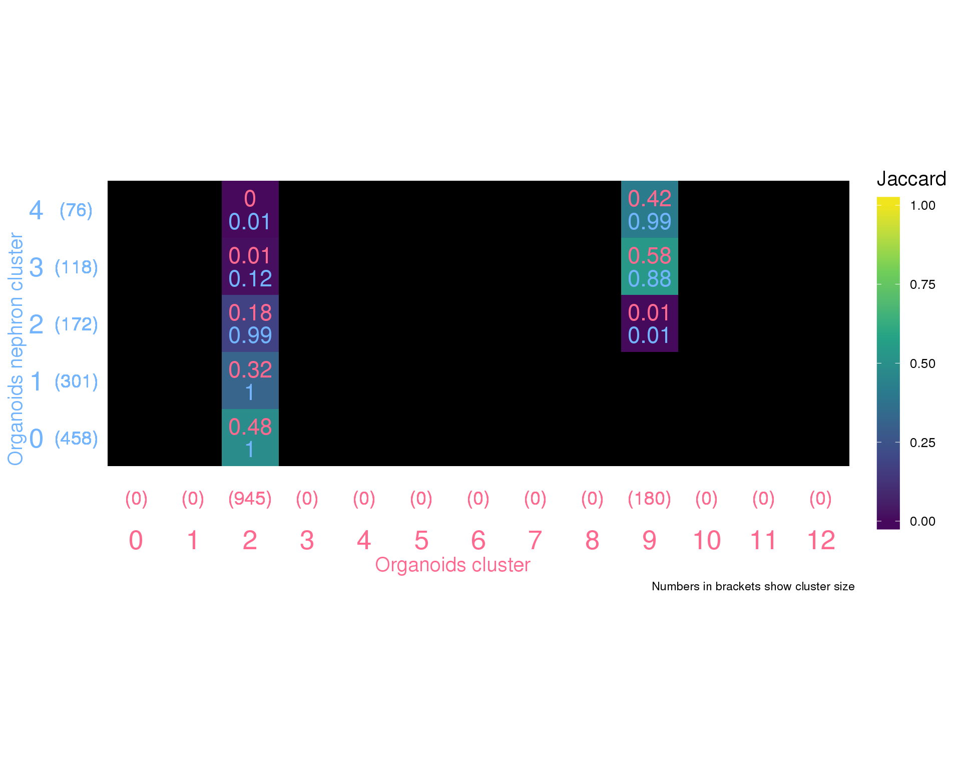
vs Combined
summariseClusts(clusts, Organoids, Combined) %>%
    ggplot(aes(x = Organoids, y = Combined, fill = Jaccard)) +
    geom_tile() +
    geom_text(aes(label = round(OrganoidsPct, 2)), nudge_y = 0.2,
              colour = "#ff698f", size = 4) +
    geom_text(aes(label = round(CombinedPct, 2)), nudge_y = -0.2,
              colour = "#73b4ff", size = 4) +
    geom_text(aes(label = glue("({OrganoidsTotal})")), y = -0.05,
              size = 3.5, colour = "#ff698f") +
    geom_text(aes(label = glue("({CombinedTotal})")), x = -0.05,
              size = 3.5, colour = "#73b4ff") +
    scale_fill_viridis_c(begin = 0.02, end = 0.98, na.value = "black",
                         limits = c(0, 1)) +
    coord_equal() +
    expand_limits(x = -0.5, y = -0.5) +
    labs(x = "Organoids cluster",
         y = "Combined cluster",
         caption = "Numbers in brackets show cluster size") +
    theme_minimal() +
    theme(axis.text = element_text(size = 20),
          axis.text.x = element_text(colour = "#ff698f"),
          axis.text.y = element_text(colour = "#73b4ff"),
          axis.ticks = element_blank(),
          axis.title = element_text(size = 15),
          axis.title.x = element_text(colour = "#ff698f"),
          axis.title.y = element_text(colour = "#73b4ff"),
          legend.key.height = unit(50, "pt"),
          legend.title = element_text(size = 15),
          legend.text = element_text(size = 10),
          panel.grid = element_blank())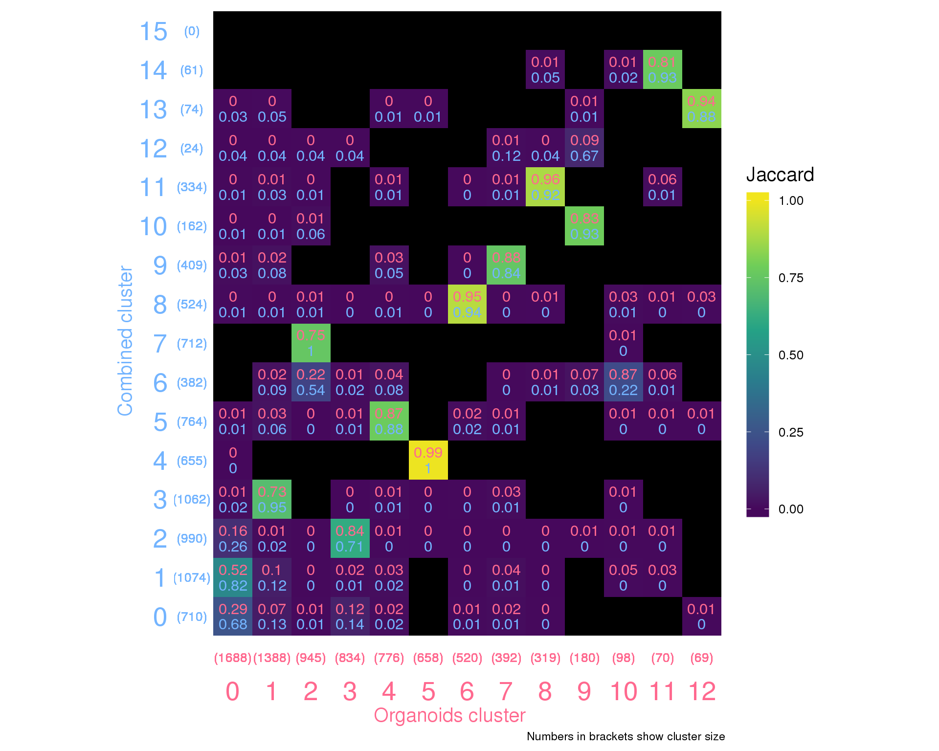
vs Combined Nephron
summariseClusts(clusts, Organoids, CombNephron) %>%
    ggplot(aes(x = Organoids, y = CombNephron, fill = Jaccard)) +
    geom_tile() +
    geom_text(aes(label = round(OrganoidsPct, 2)), nudge_y = 0.2,
              colour = "#ff698f", size = 6) +
    geom_text(aes(label = round(CombNephronPct, 2)), nudge_y = -0.2,
              colour = "#73b4ff", size = 6) +
    geom_text(aes(label = glue("({OrganoidsTotal})")), y = -0.05,
              size = 5, colour = "#ff698f") +
    geom_text(aes(label = glue("({CombNephronTotal})")), x = -0.05,
              size = 5, colour = "#73b4ff") +
    scale_fill_viridis_c(begin = 0.02, end = 0.98, na.value = "black",
                         limits = c(0, 1)) +
    coord_equal() +
    expand_limits(x = -0.5, y = -0.5) +
    labs(x = "Organoids cluster",
         y = "Combined nephron cluster",
         caption = "Numbers in brackets show cluster size") +
    theme_minimal() +
    theme(axis.text = element_text(size = 20),
          axis.text.x = element_text(colour = "#ff698f"),
          axis.text.y = element_text(colour = "#73b4ff"),
          axis.ticks = element_blank(),
          axis.title = element_text(size = 15),
          axis.title.x = element_text(colour = "#ff698f"),
          axis.title.y = element_text(colour = "#73b4ff"),
          legend.key.height = unit(50, "pt"),
          legend.title = element_text(size = 15),
          legend.text = element_text(size = 10),
          panel.grid = element_blank())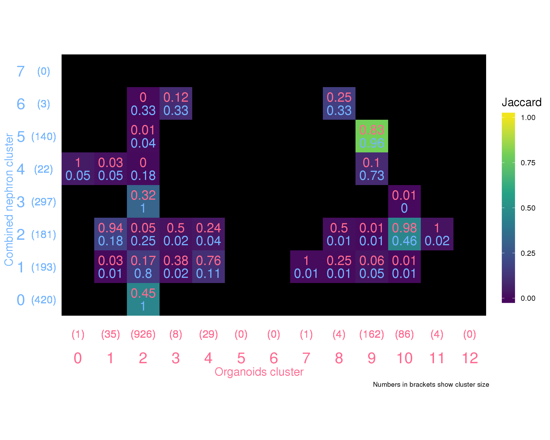
Combined
vs Combined Nephron
summariseClusts(clusts, Combined, CombNephron) %>%
    ggplot(aes(x = Combined, y = CombNephron, fill = Jaccard)) +
    geom_tile() +
    geom_text(aes(label = round(CombinedPct, 2)), nudge_y = 0.2,
              colour = "#ff698f", size = 6) +
    geom_text(aes(label = round(CombNephronPct, 2)), nudge_y = -0.2,
              colour = "#73b4ff", size = 6) +
    geom_text(aes(label = glue("({CombinedTotal})")), y = -0.05,
              size = 5, colour = "#ff698f") +
    geom_text(aes(label = glue("({CombNephronTotal})")), x = -0.05,
              size = 5, colour = "#73b4ff") +
    scale_fill_viridis_c(begin = 0.02, end = 0.98, na.value = "black",
                         limits = c(0, 1)) +
    coord_equal() +
    expand_limits(x = -0.5, y = -0.5) +
    labs(x = "Combined cluster",
         y = "Combined nephron cluster",
         caption = "Numbers in brackets show cluster size") +
    theme_minimal() +
    theme(axis.text = element_text(size = 20),
          axis.text.x = element_text(colour = "#ff698f"),
          axis.text.y = element_text(colour = "#73b4ff"),
          axis.ticks = element_blank(),
          axis.title = element_text(size = 15),
          axis.title.x = element_text(colour = "#ff698f"),
          axis.title.y = element_text(colour = "#73b4ff"),
          legend.key.height = unit(50, "pt"),
          legend.title = element_text(size = 15),
          legend.text = element_text(size = 10),
          panel.grid = element_blank())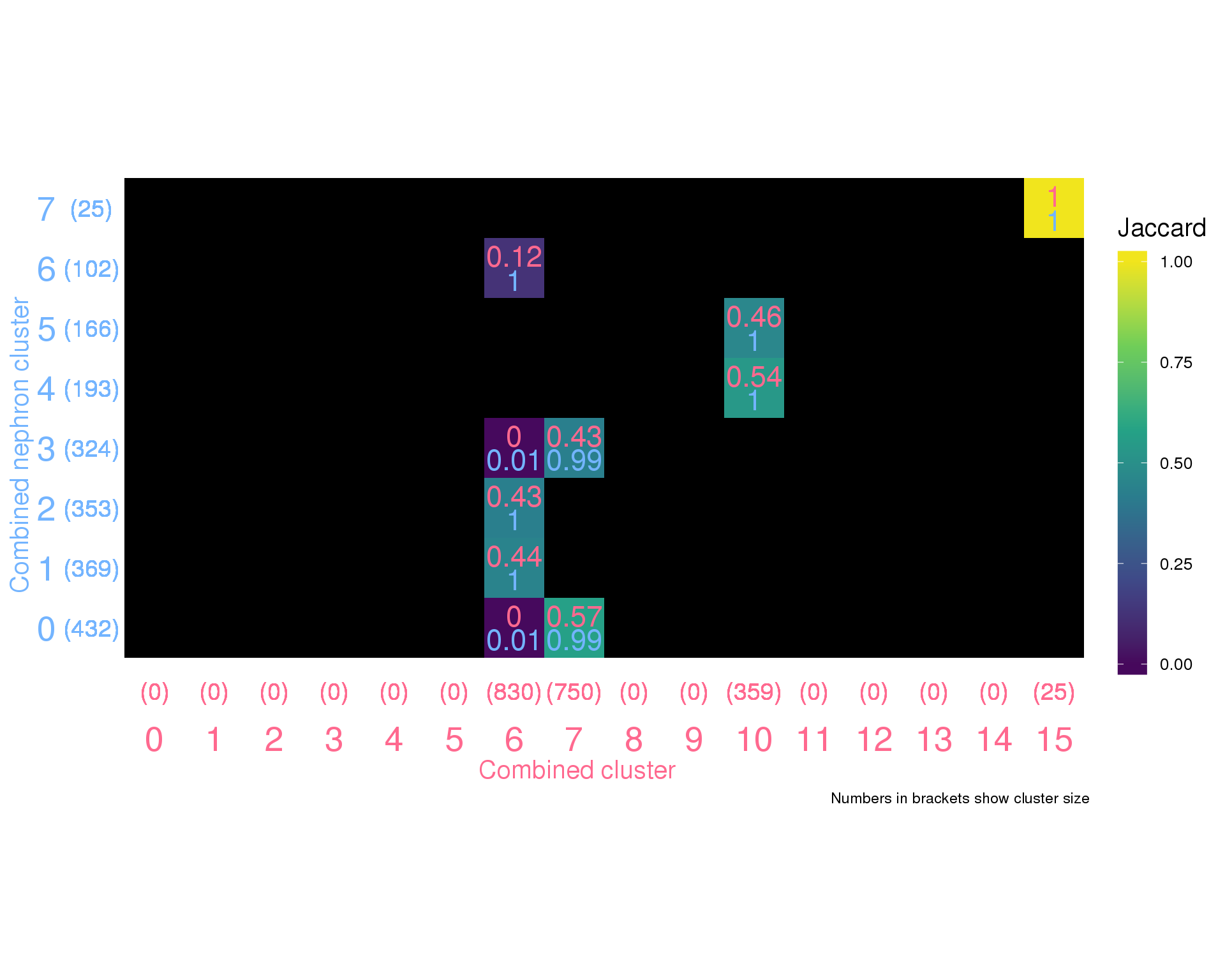
vs Organoids
summariseClusts(clusts, Combined, Organoids) %>%
    ggplot(aes(x = Combined, y = Organoids, fill = Jaccard)) +
    geom_tile() +
    geom_text(aes(label = round(CombinedPct, 2)), nudge_y = 0.2,
              colour = "#ff698f", size = 4) +
    geom_text(aes(label = round(OrganoidsPct, 2)), nudge_y = -0.2,
              colour = "#73b4ff", size = 4) +
    geom_text(aes(label = glue("({CombinedTotal})")), y = -0.05,
              size = 4, colour = "#ff698f") +
    geom_text(aes(label = glue("({OrganoidsTotal})")), x = -0.05,
              size = 4, colour = "#73b4ff") +
    scale_fill_viridis_c(begin = 0.02, end = 0.98, na.value = "black",
                         limits = c(0, 1)) +
    coord_equal() +
    expand_limits(x = -0.5, y = -0.5) +
    labs(x = "Combined cluster",
         y = "Organoids cluster",
         caption = "Numbers in brackets show cluster size") +
    theme_minimal() +
    theme(axis.text = element_text(size = 20),
          axis.text.x = element_text(colour = "#ff698f"),
          axis.text.y = element_text(colour = "#73b4ff"),
          axis.ticks = element_blank(),
          axis.title = element_text(size = 15),
          axis.title.x = element_text(colour = "#ff698f"),
          axis.title.y = element_text(colour = "#73b4ff"),
          legend.key.height = unit(50, "pt"),
          legend.title = element_text(size = 15),
          legend.text = element_text(size = 10),
          panel.grid = element_blank())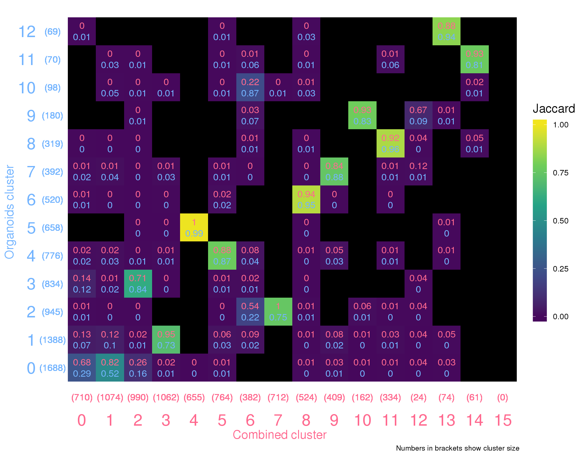
vs Organoids Nephron
summariseClusts(clusts, Combined, OrgsNephron) %>%
    ggplot(aes(x = Combined, y = OrgsNephron, fill = Jaccard)) +
    geom_tile() +
    geom_text(aes(label = round(CombinedPct, 2)), nudge_y = 0.2,
              colour = "#ff698f", size = 6) +
    geom_text(aes(label = round(OrgsNephronPct, 2)), nudge_y = -0.2,
              colour = "#73b4ff", size = 6) +
    geom_text(aes(label = glue("({CombinedTotal})")), y = -0.05,
              size = 5, colour = "#ff698f") +
    geom_text(aes(label = glue("({OrgsNephronTotal})")), x = -0.05,
              size = 5, colour = "#73b4ff") +
    scale_fill_viridis_c(begin = 0.02, end = 0.98, na.value = "black",
                         limits = c(0, 1)) +
    coord_equal() +
    expand_limits(x = -0.5, y = -0.5) +
    labs(x = "Combined cluster",
         y = "Organoids nephron cluster",
         caption = "Numbers in brackets show cluster size") +
    theme_minimal() +
    theme(axis.text = element_text(size = 20),
          axis.text.x = element_text(colour = "#ff698f"),
          axis.text.y = element_text(colour = "#73b4ff"),
          axis.ticks = element_blank(),
          axis.title = element_text(size = 15),
          axis.title.x = element_text(colour = "#ff698f"),
          axis.title.y = element_text(colour = "#73b4ff"),
          legend.key.height = unit(50, "pt"),
          legend.title = element_text(size = 15),
          legend.text = element_text(size = 10),
          panel.grid = element_blank())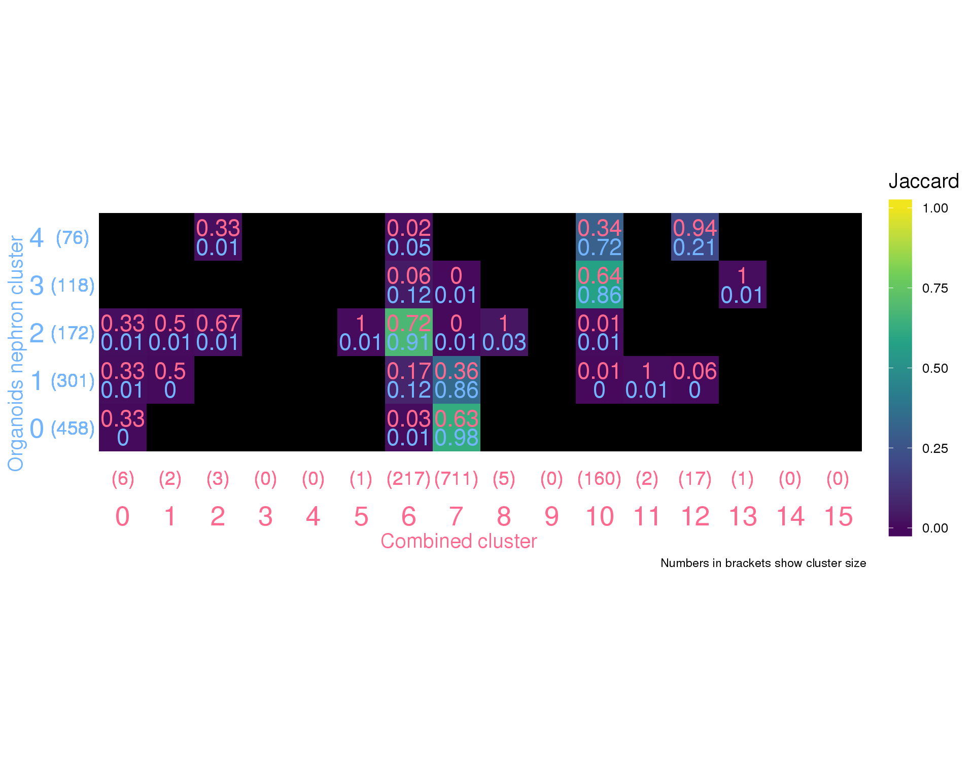
Combined nephron
vs Organoids Nephron
summariseClusts(clusts, CombNephron, OrgsNephron) %>%
    ggplot(aes(x = CombNephron, y = OrgsNephron, fill = Jaccard)) +
    geom_tile() +
    geom_text(aes(label = round(CombNephronPct, 2)), nudge_y = 0.2,
              colour = "#ff698f", size = 6) +
    geom_text(aes(label = round(OrgsNephronPct, 2)), nudge_y = -0.2,
              colour = "#73b4ff", size = 6) +
    geom_text(aes(label = glue("({CombNephronTotal})")), y = -0.05,
              size = 5, colour = "#ff698f") +
    geom_text(aes(label = glue("({OrgsNephronTotal})")), x = -0.05,
              size = 5, colour = "#73b4ff") +
    scale_fill_viridis_c(begin = 0.02, end = 0.98, na.value = "black",
                         limits = c(0, 1)) +
    coord_equal() +
    expand_limits(x = -0.5, y = -0.5) +
    labs(x = "Combined nephron cluster",
         y = "Organoids nephron cluster",
         caption = "Numbers in brackets show cluster size") +
    theme_minimal() +
    theme(axis.text = element_text(size = 20),
          axis.text.x = element_text(colour = "#ff698f"),
          axis.text.y = element_text(colour = "#73b4ff"),
          axis.ticks = element_blank(),
          axis.title = element_text(size = 15),
          axis.title.x = element_text(colour = "#ff698f"),
          axis.title.y = element_text(colour = "#73b4ff"),
          legend.key.height = unit(50, "pt"),
          legend.title = element_text(size = 15),
          legend.text = element_text(size = 10),
          panel.grid = element_blank())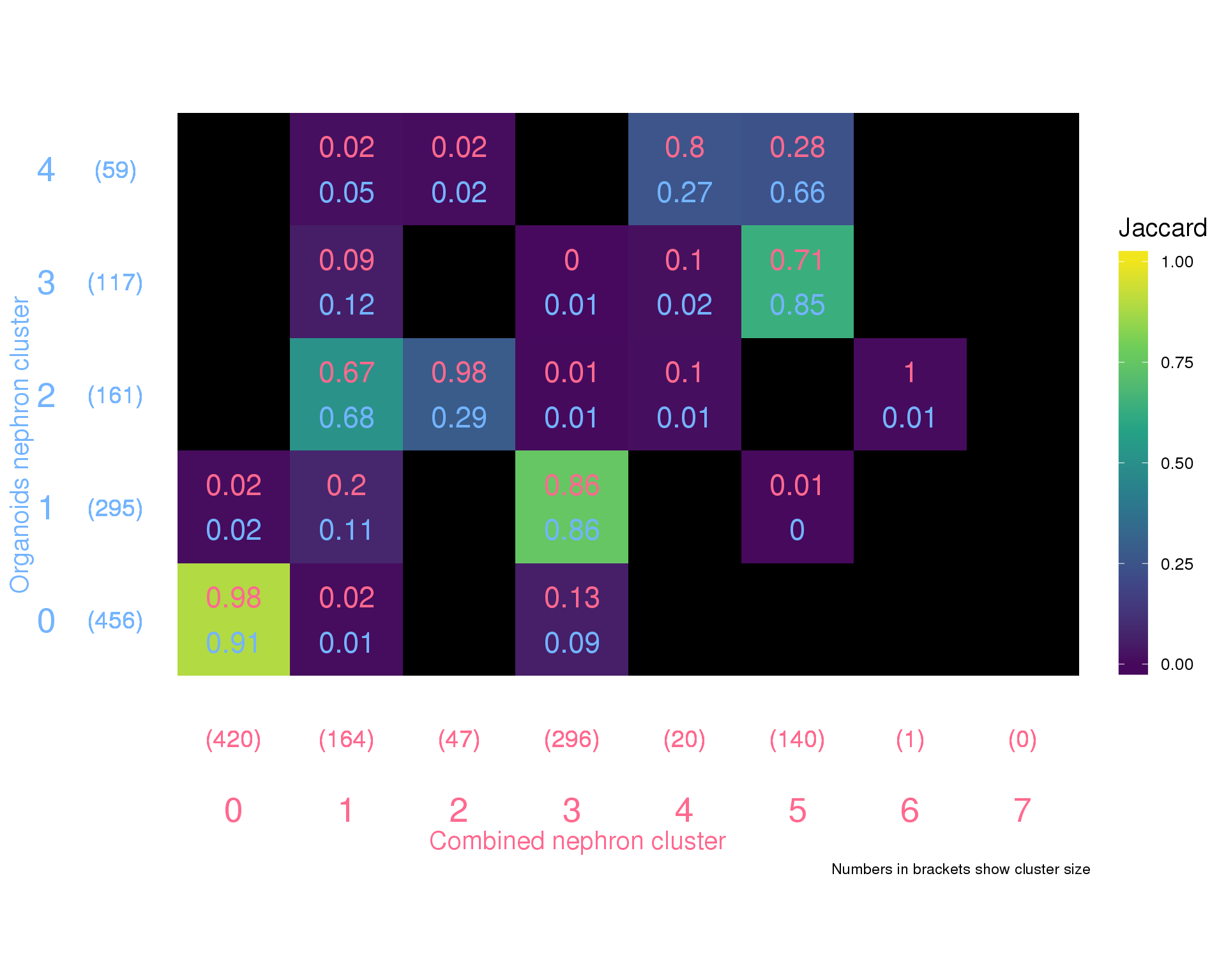
Summary
Output files
This table describes the output files produced by this document. Right click and Save Link As… to download the results.
dir.create(here("output", DOCNAME), showWarnings = FALSE)

write_csv(clusts, here("output", DOCNAME, "cluster_assignments.csv"))

kable(data.frame(
    File = c(
        glue("[cluster_assignments.csv]",
             "({getDownloadURL('cluster_assignments.csv', DOCNAME)})")
    ),
    Description = c(
        "Cluster assignments for all clustering analyses"
    )
))| File | Description |
|---|---|
| cluster_assignments.csv | Cluster assignments for all clustering analyses |
Session information
devtools::session_info() setting value
version R version 3.5.0 (2018-04-23)
system x86_64, linux-gnu
ui X11
language (EN)
collate en_US.UTF-8
tz Australia/Melbourne
date 2018-11-23
package * version date source
assertthat 0.2.0 2017-04-11 CRAN (R 3.5.0)
backports 1.1.2 2017-12-13 CRAN (R 3.5.0)
base * 3.5.0 2018-06-18 local
bindr 0.1.1 2018-03-13 cran (@0.1.1)
bindrcpp * 0.2.2 2018-03-29 cran (@0.2.2)
broom 0.5.0 2018-07-17 cran (@0.5.0)
cellranger 1.1.0 2016-07-27 CRAN (R 3.5.0)
cli 1.0.0 2017-11-05 CRAN (R 3.5.0)
colorspace 1.3-2 2016-12-14 cran (@1.3-2)
compiler 3.5.0 2018-06-18 local
crayon 1.3.4 2017-09-16 CRAN (R 3.5.0)
datasets * 3.5.0 2018-06-18 local
devtools 1.13.6 2018-06-27 CRAN (R 3.5.0)
digest 0.6.15 2018-01-28 CRAN (R 3.5.0)
dplyr * 0.7.6 2018-06-29 cran (@0.7.6)
evaluate 0.10.1 2017-06-24 CRAN (R 3.5.0)
forcats * 0.3.0 2018-02-19 CRAN (R 3.5.0)
ggplot2 * 3.0.0 2018-07-03 cran (@3.0.0)
git2r 0.21.0 2018-01-04 CRAN (R 3.5.0)
glue * 1.3.0 2018-07-17 cran (@1.3.0)
graphics * 3.5.0 2018-06-18 local
grDevices * 3.5.0 2018-06-18 local
grid 3.5.0 2018-06-18 local
gtable 0.2.0 2016-02-26 cran (@0.2.0)
haven 1.1.2 2018-06-27 CRAN (R 3.5.0)
here * 0.1 2017-05-28 CRAN (R 3.5.0)
highr 0.7 2018-06-09 CRAN (R 3.5.0)
hms 0.4.2 2018-03-10 CRAN (R 3.5.0)
htmltools 0.3.6 2017-04-28 CRAN (R 3.5.0)
httr 1.3.1 2017-08-20 CRAN (R 3.5.0)
jsonlite 1.5 2017-06-01 CRAN (R 3.5.0)
knitr * 1.20 2018-02-20 CRAN (R 3.5.0)
labeling 0.3 2014-08-23 cran (@0.3)
lattice 0.20-35 2017-03-25 CRAN (R 3.5.0)
lazyeval 0.2.1 2017-10-29 cran (@0.2.1)
lubridate 1.7.4 2018-04-11 cran (@1.7.4)
magrittr 1.5 2014-11-22 CRAN (R 3.5.0)
memoise 1.1.0 2017-04-21 CRAN (R 3.5.0)
methods * 3.5.0 2018-06-18 local
modelr 0.1.2 2018-05-11 CRAN (R 3.5.0)
munsell 0.5.0 2018-06-12 cran (@0.5.0)
nlme 3.1-137 2018-04-07 CRAN (R 3.5.0)
pillar 1.3.0 2018-07-14 cran (@1.3.0)
pkgconfig 2.0.1 2017-03-21 cran (@2.0.1)
plyr 1.8.4 2016-06-08 cran (@1.8.4)
purrr * 0.2.5 2018-05-29 cran (@0.2.5)
R.methodsS3 1.7.1 2016-02-16 CRAN (R 3.5.0)
R.oo 1.22.0 2018-04-22 CRAN (R 3.5.0)
R.utils 2.6.0 2017-11-05 CRAN (R 3.5.0)
R6 2.2.2 2017-06-17 CRAN (R 3.5.0)
Rcpp 0.12.18 2018-07-23 cran (@0.12.18)
readr * 1.1.1 2017-05-16 CRAN (R 3.5.0)
readxl 1.1.0 2018-04-20 CRAN (R 3.5.0)
rlang 0.2.1 2018-05-30 CRAN (R 3.5.0)
rmarkdown 1.10.2 2018-07-30 Github (rstudio/rmarkdown@18207b9)
rprojroot 1.3-2 2018-01-03 CRAN (R 3.5.0)
rstudioapi 0.7 2017-09-07 CRAN (R 3.5.0)
rvest 0.3.2 2016-06-17 CRAN (R 3.5.0)
scales 0.5.0 2017-08-24 cran (@0.5.0)
stats * 3.5.0 2018-06-18 local
stringi 1.2.4 2018-07-20 cran (@1.2.4)
stringr * 1.3.1 2018-05-10 CRAN (R 3.5.0)
tibble * 1.4.2 2018-01-22 cran (@1.4.2)
tidyr * 0.8.1 2018-05-18 cran (@0.8.1)
tidyselect 0.2.4 2018-02-26 cran (@0.2.4)
tidyverse * 1.2.1 2017-11-14 CRAN (R 3.5.0)
tools 3.5.0 2018-06-18 local
utils * 3.5.0 2018-06-18 local
viridisLite 0.3.0 2018-02-01 cran (@0.3.0)
whisker 0.3-2 2013-04-28 CRAN (R 3.5.0)
withr 2.1.2 2018-03-15 CRAN (R 3.5.0)
workflowr 1.1.1 2018-07-06 CRAN (R 3.5.0)
xml2 1.2.0 2018-01-24 CRAN (R 3.5.0)
yaml 2.2.0 2018-07-25 cran (@2.2.0) This reproducible R Markdown analysis was created with workflowr 1.1.1