Combined Clustering
Last updated: 2018-12-05
workflowr checks: (Click a bullet for more information)-
✔ R Markdown file: up-to-date
Great! Since the R Markdown file has been committed to the Git repository, you know the exact version of the code that produced these results.
-
✔ Environment: empty
Great job! The global environment was empty. Objects defined in the global environment can affect the analysis in your R Markdown file in unknown ways. For reproduciblity it’s best to always run the code in an empty environment.
-
✔ Seed:
set.seed(20180730)The command
set.seed(20180730)was run prior to running the code in the R Markdown file. Setting a seed ensures that any results that rely on randomness, e.g. subsampling or permutations, are reproducible. -
✔ Session information: recorded
Great job! Recording the operating system, R version, and package versions is critical for reproducibility.
-
Great! You are using Git for version control. Tracking code development and connecting the code version to the results is critical for reproducibility. The version displayed above was the version of the Git repository at the time these results were generated.✔ Repository version: bd6173a
Note that you need to be careful to ensure that all relevant files for the analysis have been committed to Git prior to generating the results (you can usewflow_publishorwflow_git_commit). workflowr only checks the R Markdown file, but you know if there are other scripts or data files that it depends on. Below is the status of the Git repository when the results were generated:
Note that any generated files, e.g. HTML, png, CSS, etc., are not included in this status report because it is ok for generated content to have uncommitted changes.Ignored files: Ignored: .DS_Store Ignored: .Rhistory Ignored: .Rproj.user/ Ignored: analysis/cache.bak.20181031/ Ignored: analysis/cache.bak/ Ignored: analysis/cache.lind2.20181114/ Ignored: analysis/cache/ Ignored: data/Lindstrom2/ Ignored: data/processed.bak.20181031/ Ignored: data/processed.bak/ Ignored: data/processed.lind2.20181114/ Ignored: output/04B_Organoids_Nephron/cluster_de.csv.zip Ignored: output/04B_Organoids_Nephron/conserved_markers.csv.zip Ignored: output/04B_Organoids_Nephron/markers.csv.zip Ignored: output/04_Organoids_Clustering/cluster_de.csv.zip Ignored: output/04_Organoids_Clustering/conserved_markers.csv.zip Ignored: output/04_Organoids_Clustering/markers.csv.zip Ignored: output/07B_Combined_Nephron/cluster_de.csv.zip Ignored: output/07B_Combined_Nephron/cluster_de_filtered.csv.zip Ignored: output/07B_Combined_Nephron/conserved_markers.csv.zip Ignored: output/07B_Combined_Nephron/markers.csv.zip Ignored: output/07B_Combined_Nephron/podocyte_de.csv.zip Ignored: output/07B_Combined_Nephron/podocyte_de_filtered.csv.zip Ignored: output/07_Combined_Clustering/cluster_de.csv.zip Ignored: output/07_Combined_Clustering/cluster_de_filtered.csv.zip Ignored: output/07_Combined_Clustering/conserved_markers.csv.zip Ignored: output/07_Combined_Clustering/group_de.csv.zip Ignored: output/07_Combined_Clustering/markers.csv.zip Ignored: packrat/lib-R/ Ignored: packrat/lib-ext/ Ignored: packrat/lib/ Ignored: packrat/src/ Ignored: test.csv.zip Unstaged changes: Deleted: output/04B_Organoids_Nephron/cluster_de.csv Modified: output/04B_Organoids_Nephron/cluster_de.xlsx Deleted: output/04B_Organoids_Nephron/conserved_markers.csv Modified: output/04B_Organoids_Nephron/conserved_markers.xlsx Deleted: output/04B_Organoids_Nephron/markers.csv Modified: output/04B_Organoids_Nephron/markers.xlsx Deleted: output/04_Organoids_Clustering/cluster_de.csv Modified: output/04_Organoids_Clustering/cluster_de.xlsx Deleted: output/04_Organoids_Clustering/conserved_markers.csv Modified: output/04_Organoids_Clustering/conserved_markers.xlsx Deleted: output/04_Organoids_Clustering/markers.csv Modified: output/04_Organoids_Clustering/markers.xlsx Deleted: output/07B_Combined_Nephron/cluster_de.csv Modified: output/07B_Combined_Nephron/cluster_de.xlsx Deleted: output/07B_Combined_Nephron/cluster_de_filtered.csv Modified: output/07B_Combined_Nephron/cluster_de_filtered.xlsx Deleted: output/07B_Combined_Nephron/conserved_markers.csv Modified: output/07B_Combined_Nephron/conserved_markers.xlsx Deleted: output/07B_Combined_Nephron/markers.csv Modified: output/07B_Combined_Nephron/markers.xlsx Deleted: output/07B_Combined_Nephron/podocyte_de.csv Deleted: output/07B_Combined_Nephron/podocyte_de_filtered.csv Deleted: output/07_Combined_Clustering/cluster_de.csv Modified: output/07_Combined_Clustering/cluster_de.xlsx Deleted: output/07_Combined_Clustering/cluster_de_filtered.csv Modified: output/07_Combined_Clustering/cluster_de_filtered.xlsx Deleted: output/07_Combined_Clustering/conserved_markers.csv Modified: output/07_Combined_Clustering/conserved_markers.xlsx Deleted: output/07_Combined_Clustering/group_de.csv Deleted: output/07_Combined_Clustering/markers.csv Modified: output/07_Combined_Clustering/markers.xlsx
Expand here to see past versions:
| File | Version | Author | Date | Message |
|---|---|---|---|---|
| Rmd | bd6173a | Luke Zappia | 2018-12-05 | Add gene ids to output files |
| html | 582acea | Luke Zappia | 2018-12-03 | Fix DE results summary plot cluster labels |
| Rmd | d79b8e7 | Luke Zappia | 2018-11-20 | Create DE signature and filter results |
| html | d79b8e7 | Luke Zappia | 2018-11-20 | Create DE signature and filter results |
| html | a61f9c9 | Luke Zappia | 2018-09-13 | Rebuild site |
| html | ad10b21 | Luke Zappia | 2018-09-13 | Switch to GitHub |
| Rmd | 8fc820c | Luke Zappia | 2018-09-06 | Fix C7 C15 DE output files |
| Rmd | 6d6cabf | Luke Zappia | 2018-09-03 | Fix output file links |
| Rmd | 46fe054 | Luke Zappia | 2018-09-03 | Add C7 C15 DE |
| Rmd | bff4d5b | Luke Zappia | 2018-08-14 | Add crossover document |
# scRNA-seq
library("Seurat")
library("limma")
# Plotting
library("clustree")
library("viridis")
# Presentation
library("glue")
library("knitr")
# Parallel
library("BiocParallel")
# Paths
library("here")
# Output
library("writexl")
library("jsonlite")
# Tidyverse
library("tidyverse")source(here("R/output.R"))combined.path <- here("data/processed/Combined_Seurat.Rds")bpparam <- MulticoreParam(workers = 10)Introduction
In this document we are going to load the combined Organoids and Linstrom dataset and complete the rest of the Seurat analysis.
if (file.exists(combined.path)) {
combined <- read_rds(combined.path)
} else {
stop("Combined dataset is missing. ",
"Please run '06_Combined_Integration.Rmd' first.",
call. = FALSE)
}Clustering
Selecting resolution
n.dims <- 20
resolutions <- seq(0, 1, 0.1)
combined <- FindClusters(combined, reduction.type = "cca.aligned",
dims.use = 1:n.dims, resolution = resolutions)Seurat has a resolution parameter that indirectly controls the number of clusters it produces. We tried clustering at a range of resolutions from 0 to 1.
t-SNE plots
Here are t-SNE plots of the different clusterings.
src_list <- lapply(resolutions, function(res) {
src <- c("#### Res {{res}} {.unnumbered}",
"```{r cluster-tSNE-{{res}}}",
"TSNEPlot(combined, group.by = 'res.{{res}}', do.return = TRUE)",
"```",
"")
knit_expand(text = src)
})
out <- knit_child(text = unlist(src_list), options = list(cache = FALSE))Res 0
TSNEPlot(combined, group.by = 'res.0', do.return = TRUE)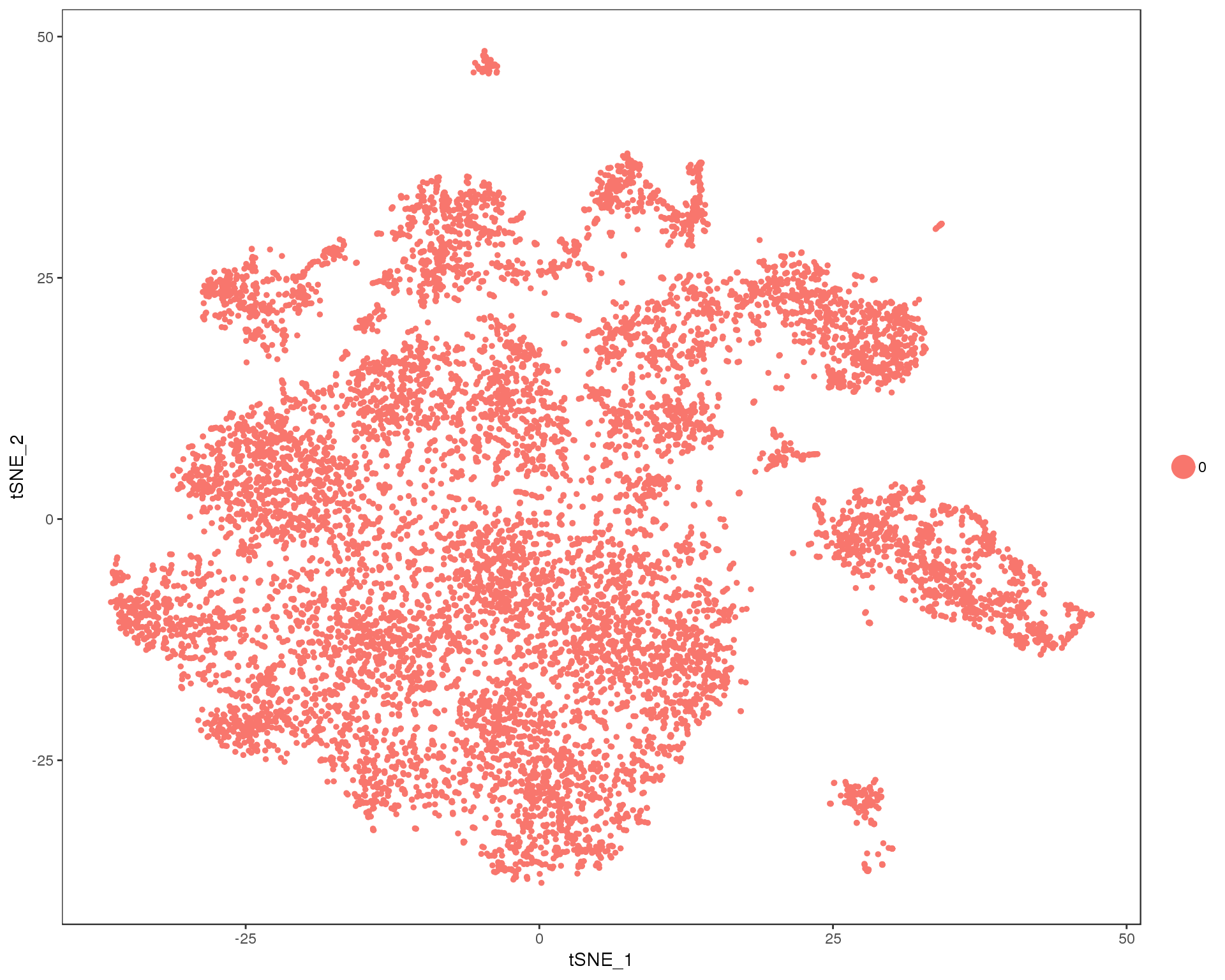
Expand here to see past versions of cluster-tSNE-0-1.png:
| Version | Author | Date |
|---|---|---|
| 5476164 | Luke Zappia | 2018-08-10 |
Res 0.1
TSNEPlot(combined, group.by = 'res.0.1', do.return = TRUE)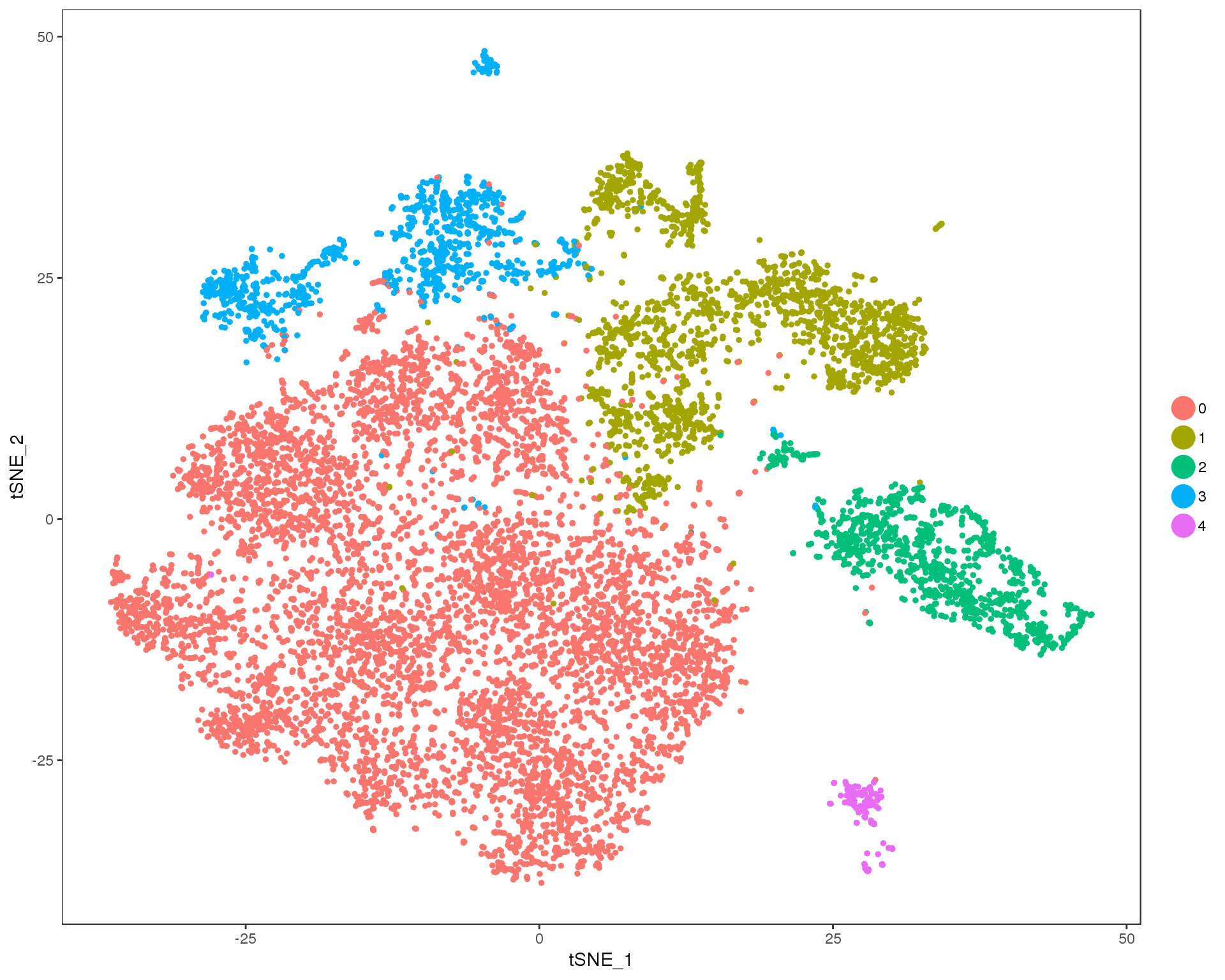
Expand here to see past versions of cluster-tSNE-0.1-1.png:
| Version | Author | Date |
|---|---|---|
| 5476164 | Luke Zappia | 2018-08-10 |
Res 0.2
TSNEPlot(combined, group.by = 'res.0.2', do.return = TRUE)
Expand here to see past versions of cluster-tSNE-0.2-1.png:
| Version | Author | Date |
|---|---|---|
| 5476164 | Luke Zappia | 2018-08-10 |
Res 0.3
TSNEPlot(combined, group.by = 'res.0.3', do.return = TRUE)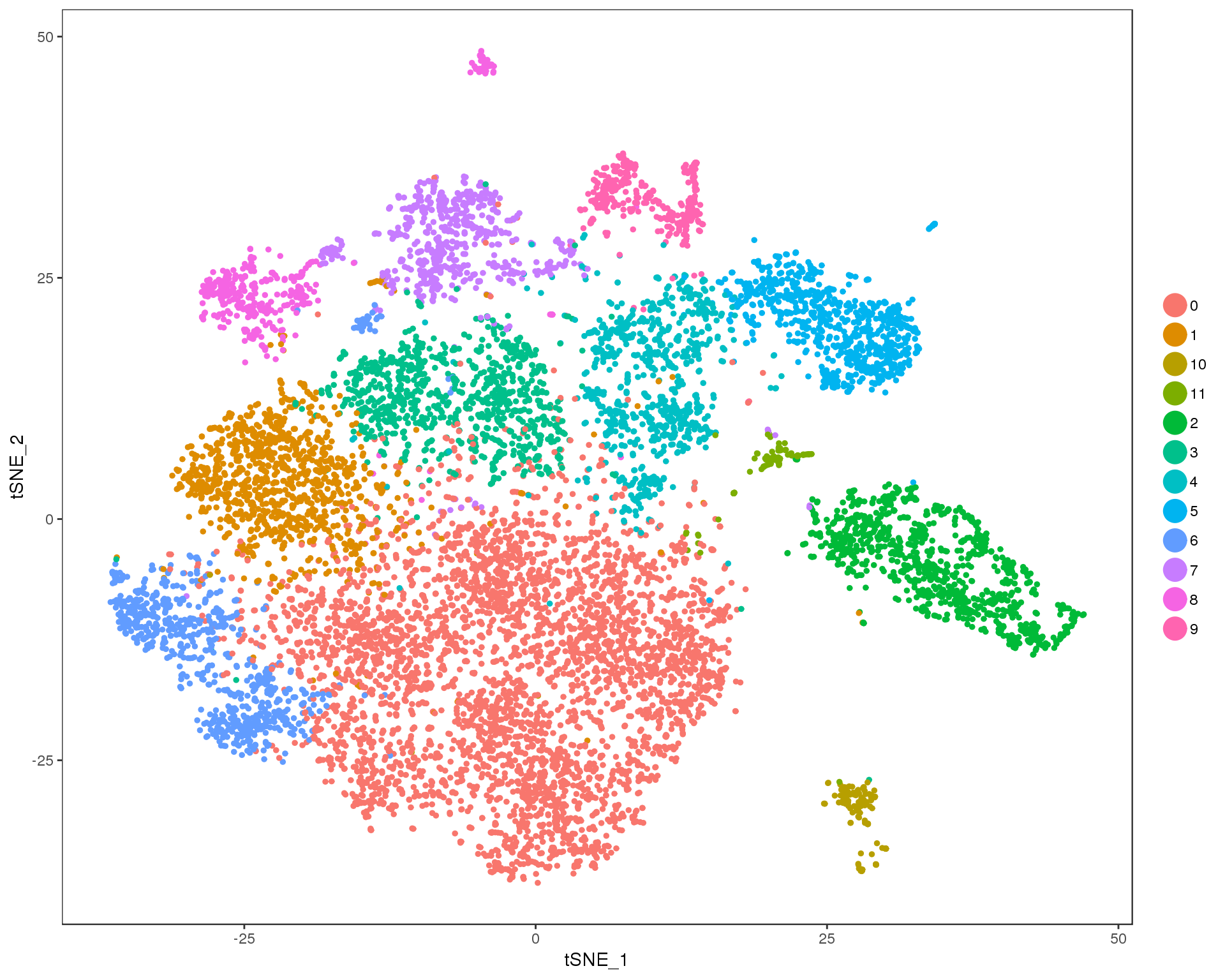
Expand here to see past versions of cluster-tSNE-0.3-1.png:
| Version | Author | Date |
|---|---|---|
| 5476164 | Luke Zappia | 2018-08-10 |
Res 0.4
TSNEPlot(combined, group.by = 'res.0.4', do.return = TRUE)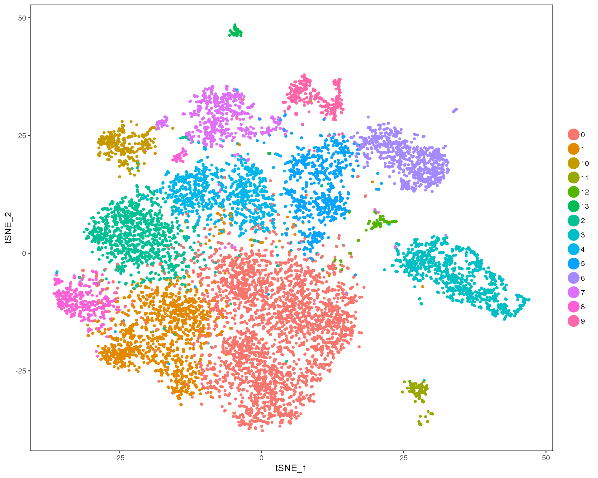
Expand here to see past versions of cluster-tSNE-0.4-1.png:
| Version | Author | Date |
|---|---|---|
| 5476164 | Luke Zappia | 2018-08-10 |
Res 0.5
TSNEPlot(combined, group.by = 'res.0.5', do.return = TRUE)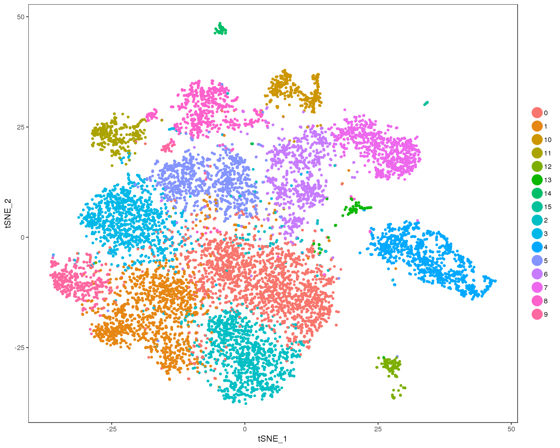
Expand here to see past versions of cluster-tSNE-0.5-1.png:
| Version | Author | Date |
|---|---|---|
| 5476164 | Luke Zappia | 2018-08-10 |
Res 0.6
TSNEPlot(combined, group.by = 'res.0.6', do.return = TRUE)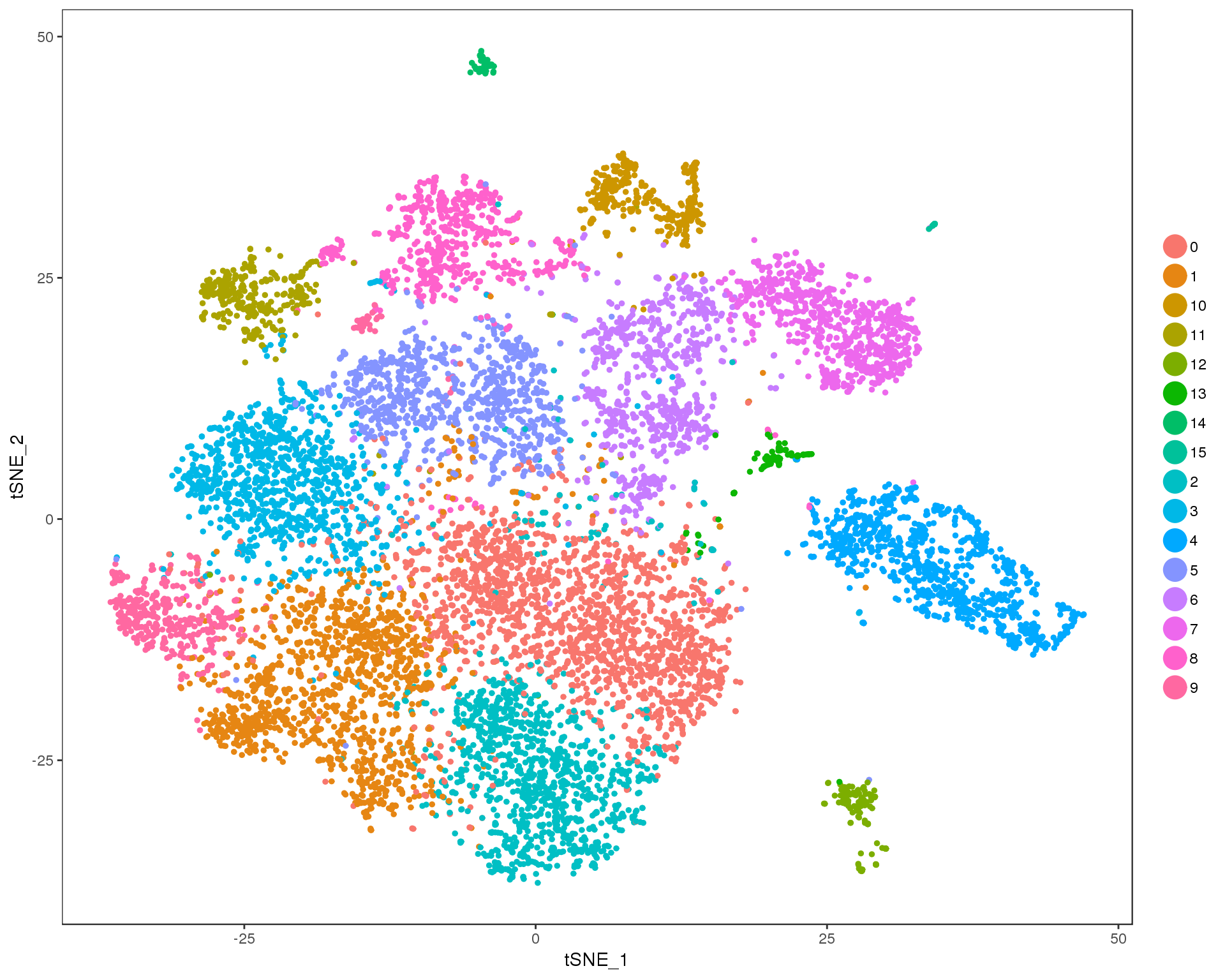
Expand here to see past versions of cluster-tSNE-0.6-1.png:
| Version | Author | Date |
|---|---|---|
| 5476164 | Luke Zappia | 2018-08-10 |
Res 0.7
TSNEPlot(combined, group.by = 'res.0.7', do.return = TRUE)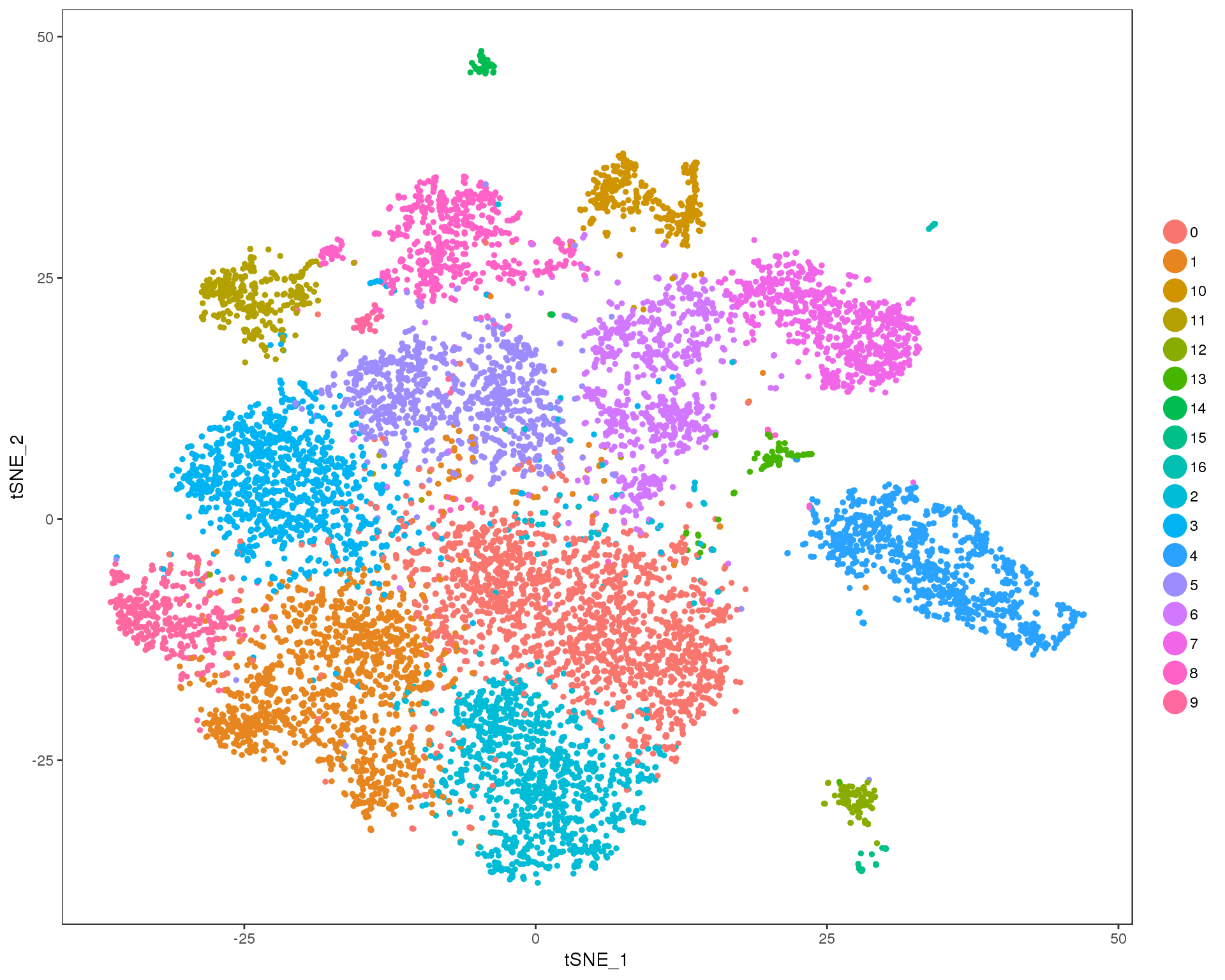
Expand here to see past versions of cluster-tSNE-0.7-1.png:
| Version | Author | Date |
|---|---|---|
| 5476164 | Luke Zappia | 2018-08-10 |
Res 0.8
TSNEPlot(combined, group.by = 'res.0.8', do.return = TRUE)
Expand here to see past versions of cluster-tSNE-0.8-1.png:
| Version | Author | Date |
|---|---|---|
| 5476164 | Luke Zappia | 2018-08-10 |
Res 0.9
TSNEPlot(combined, group.by = 'res.0.9', do.return = TRUE)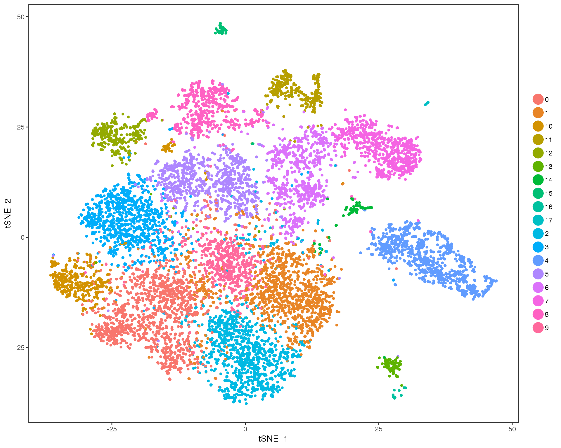
Expand here to see past versions of cluster-tSNE-0.9-1.png:
| Version | Author | Date |
|---|---|---|
| 5476164 | Luke Zappia | 2018-08-10 |
Res 1
TSNEPlot(combined, group.by = 'res.1', do.return = TRUE)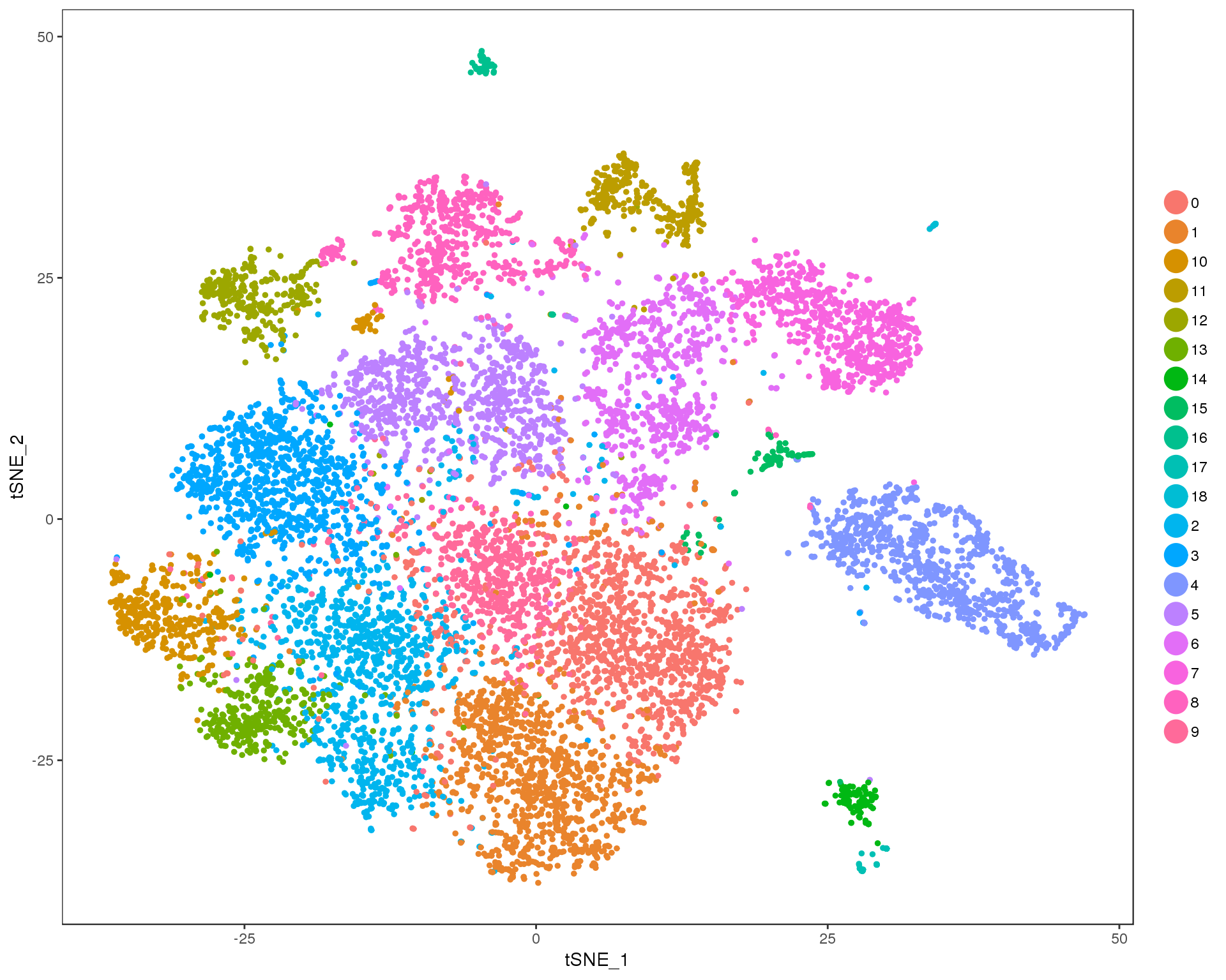
Expand here to see past versions of cluster-tSNE-1-1.png:
| Version | Author | Date |
|---|---|---|
| 5476164 | Luke Zappia | 2018-08-10 |
Clustering tree
Standard
Coloured by clustering resolution.
clustree(combined)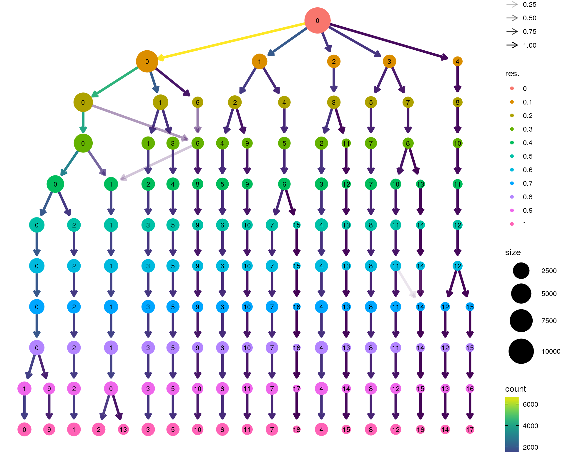
Expand here to see past versions of clustree-1.png:
| Version | Author | Date |
|---|---|---|
| 5476164 | Luke Zappia | 2018-08-10 |
Stability
Coloured by the SC3 stability metric.
clustree(combined, node_colour = "sc3_stability")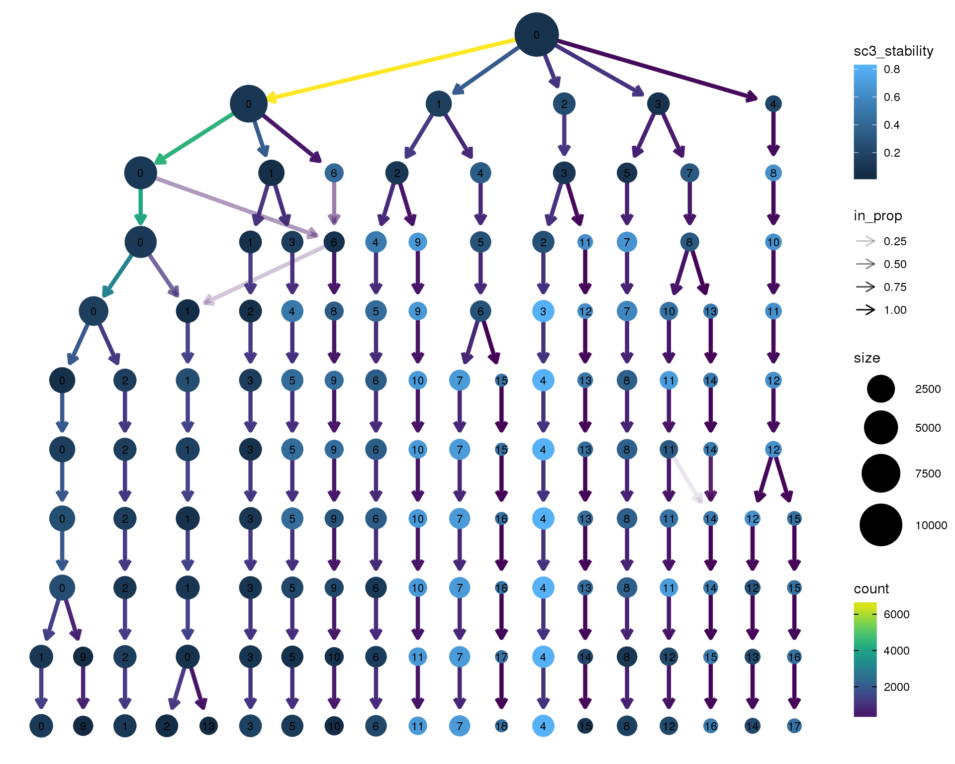
Expand here to see past versions of clustree-stability-1.png:
| Version | Author | Date |
|---|---|---|
| 5476164 | Luke Zappia | 2018-08-10 |
Gene expression
Coloured by the expression of some well-known kidney marker genes.
genes <- c("PECAM1", "CDH5", "MEIS1", "PDGFRA", "HMGB2", "CENPA", "SIX1",
"DAPL1", "NPHS1", "PODXL", "S100A8", "TYROBP", "MAL", "EMX2",
"LRP2", "GATA3", "SLC12A1", "SPINT2", "TUBB2B", "STMN2", "TTYH1",
"HBA1", "HBG1")
is_present <- genes %in% rownames(combined@data)The following genes aren’t present in this dataset and will be skipped:
src_list <- lapply(genes[is_present], function(gene) {
src <- c("##### {{gene}} {.unnumbered}",
"```{r clustree-{{gene}}}",
"clustree(combined, node_colour = '{{gene}}',",
"node_colour_aggr = 'mean',",
"exprs = 'scale.data') +",
"scale_colour_viridis_c(option = 'plasma', begin = 0.3)",
"```",
"")
knit_expand(text = src)
})
out <- knit_child(text = unlist(src_list), options = list(cache = FALSE))PECAM1
clustree(combined, node_colour = 'PECAM1',
node_colour_aggr = 'mean',
exprs = 'scale.data') +
scale_colour_viridis_c(option = 'plasma', begin = 0.3)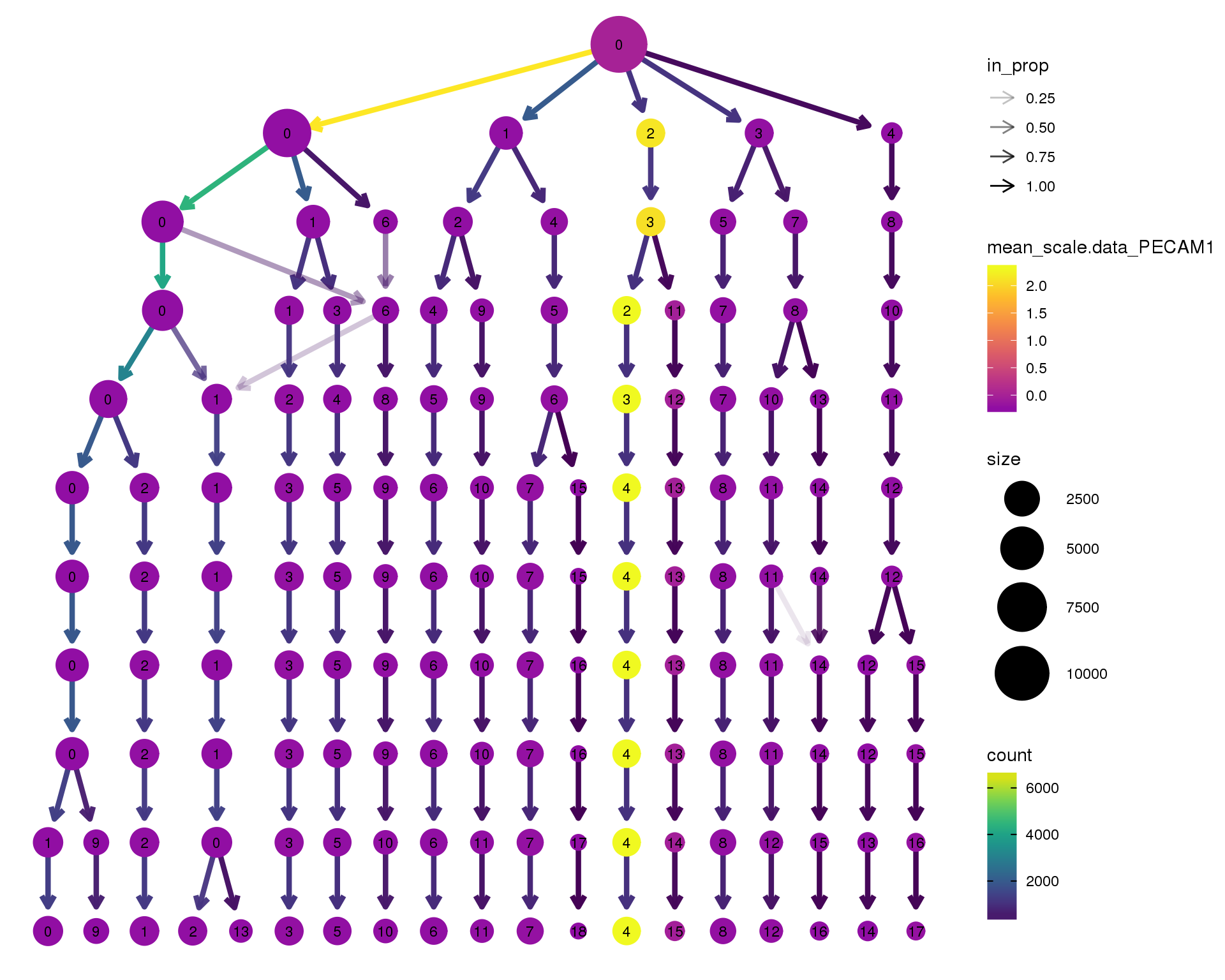
Expand here to see past versions of clustree-PECAM1-1.png:
| Version | Author | Date |
|---|---|---|
| ad10b21 | Luke Zappia | 2018-09-13 |
CDH5
clustree(combined, node_colour = 'CDH5',
node_colour_aggr = 'mean',
exprs = 'scale.data') +
scale_colour_viridis_c(option = 'plasma', begin = 0.3)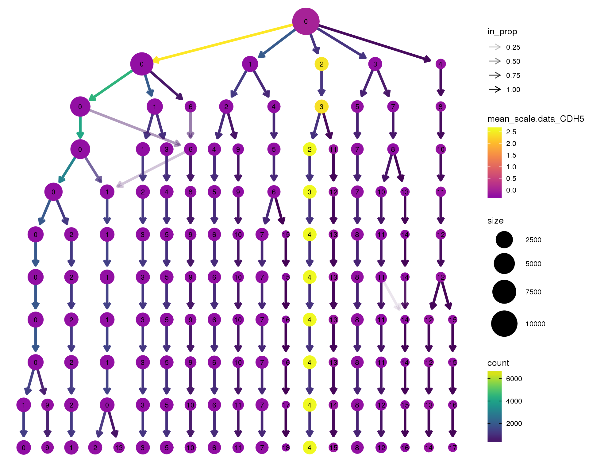
Expand here to see past versions of clustree-CDH5-1.png:
| Version | Author | Date |
|---|---|---|
| ad10b21 | Luke Zappia | 2018-09-13 |
MEIS1
clustree(combined, node_colour = 'MEIS1',
node_colour_aggr = 'mean',
exprs = 'scale.data') +
scale_colour_viridis_c(option = 'plasma', begin = 0.3)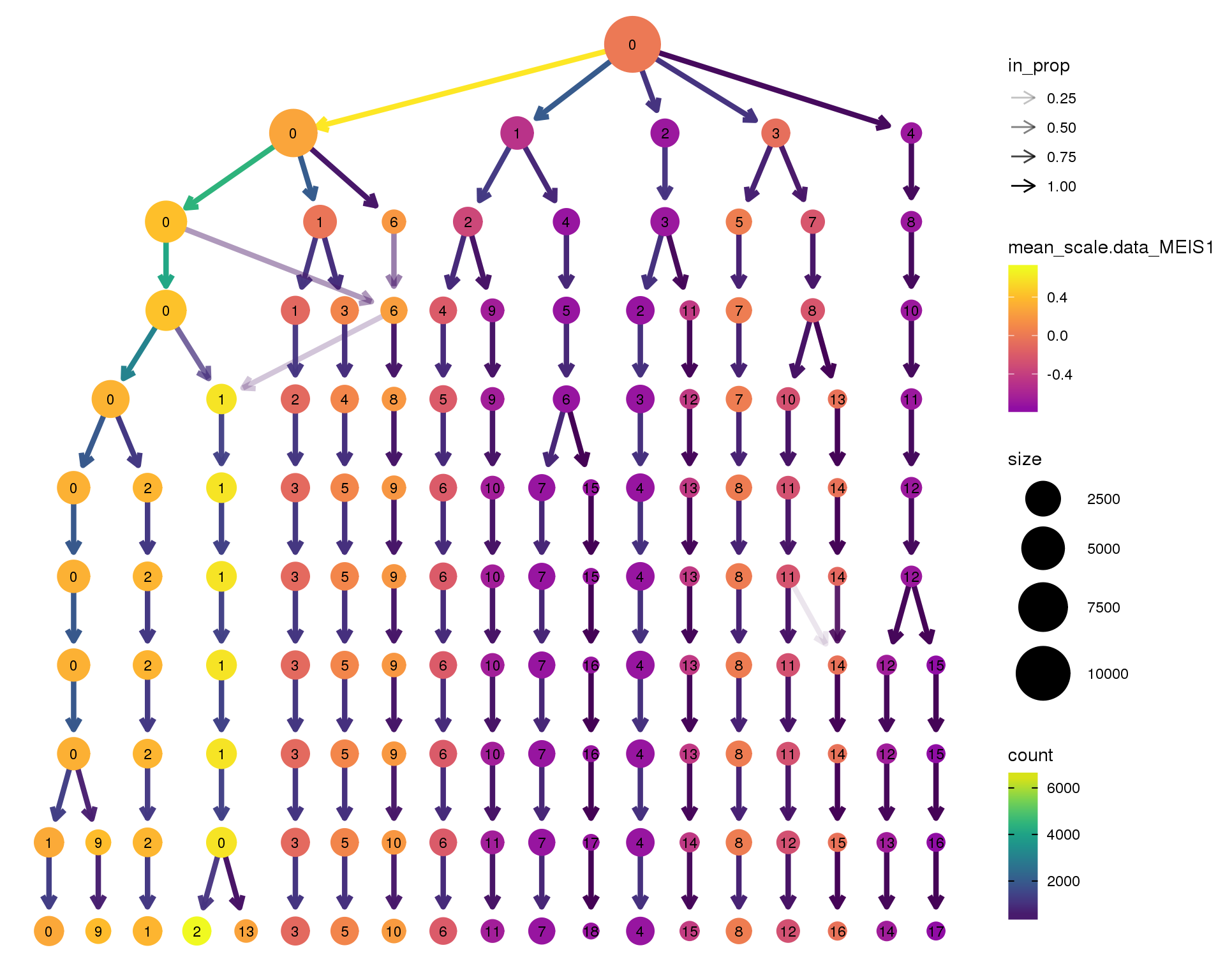
Expand here to see past versions of clustree-MEIS1-1.png:
| Version | Author | Date |
|---|---|---|
| ad10b21 | Luke Zappia | 2018-09-13 |
PDGFRA
clustree(combined, node_colour = 'PDGFRA',
node_colour_aggr = 'mean',
exprs = 'scale.data') +
scale_colour_viridis_c(option = 'plasma', begin = 0.3)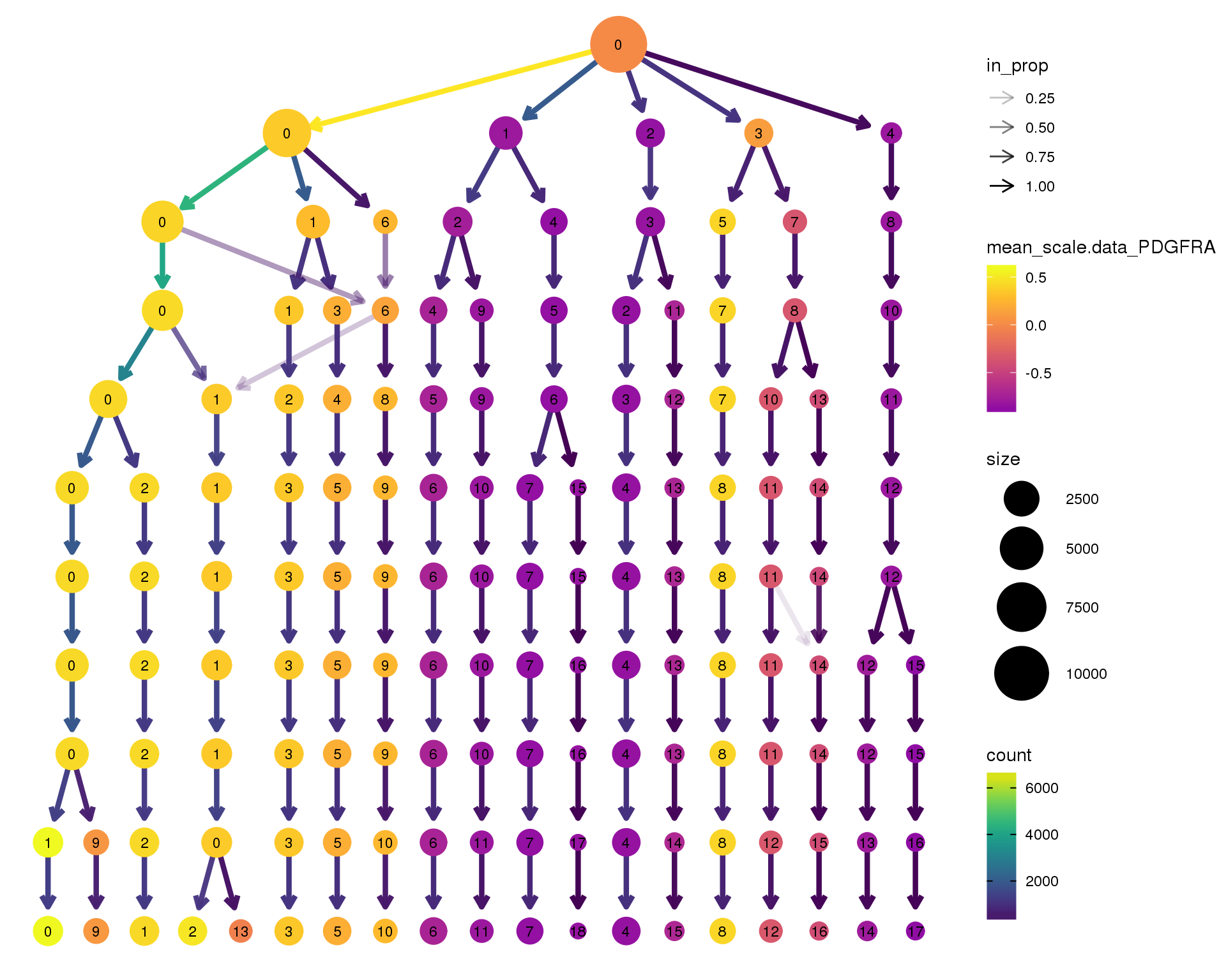
Expand here to see past versions of clustree-PDGFRA-1.png:
| Version | Author | Date |
|---|---|---|
| ad10b21 | Luke Zappia | 2018-09-13 |
HMGB2
clustree(combined, node_colour = 'HMGB2',
node_colour_aggr = 'mean',
exprs = 'scale.data') +
scale_colour_viridis_c(option = 'plasma', begin = 0.3)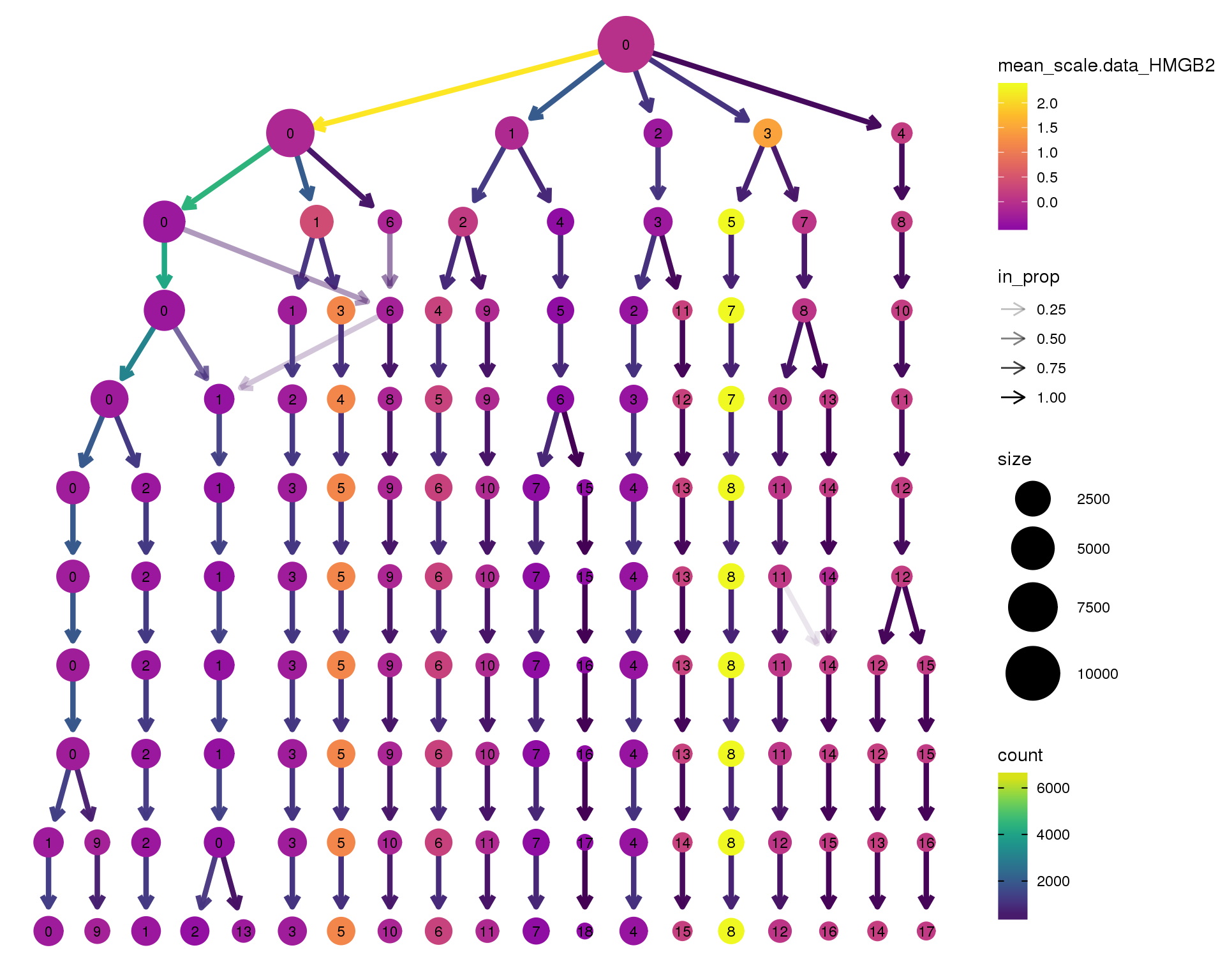
Expand here to see past versions of clustree-HMGB2-1.png:
| Version | Author | Date |
|---|---|---|
| ad10b21 | Luke Zappia | 2018-09-13 |
CENPA
clustree(combined, node_colour = 'CENPA',
node_colour_aggr = 'mean',
exprs = 'scale.data') +
scale_colour_viridis_c(option = 'plasma', begin = 0.3)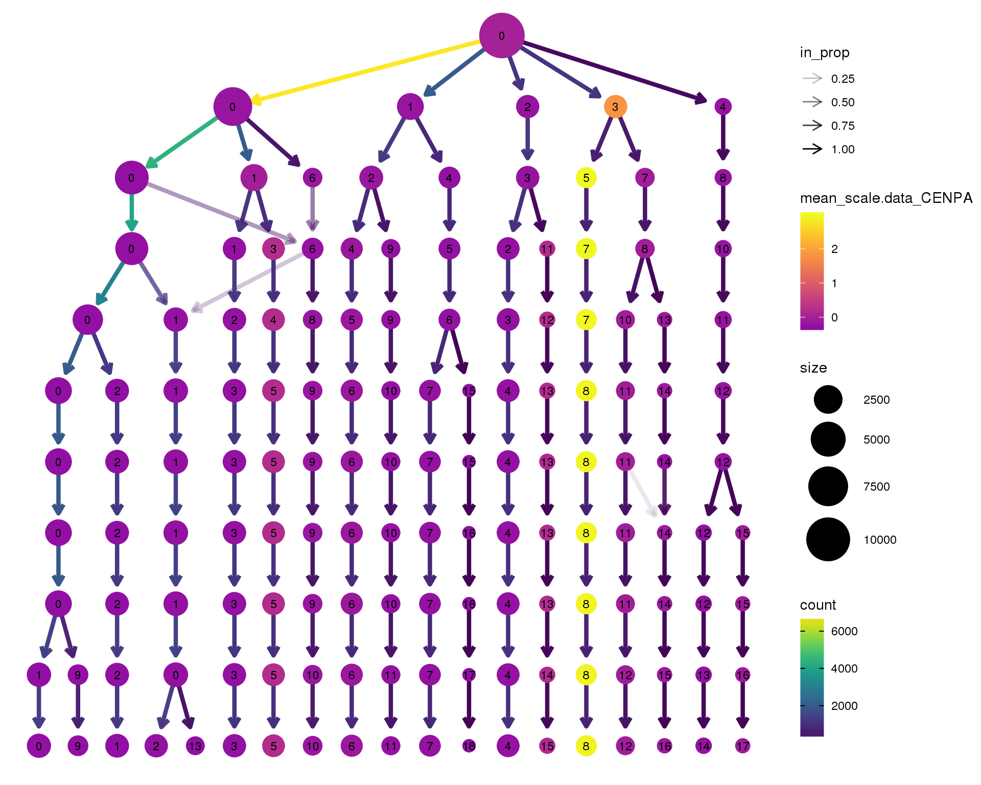
Expand here to see past versions of clustree-CENPA-1.png:
| Version | Author | Date |
|---|---|---|
| ad10b21 | Luke Zappia | 2018-09-13 |
SIX1
clustree(combined, node_colour = 'SIX1',
node_colour_aggr = 'mean',
exprs = 'scale.data') +
scale_colour_viridis_c(option = 'plasma', begin = 0.3)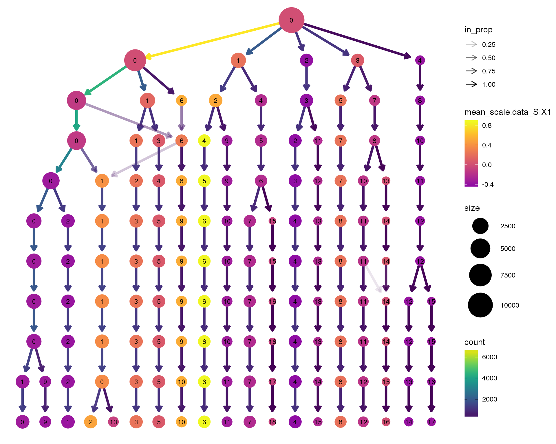
Expand here to see past versions of clustree-SIX1-1.png:
| Version | Author | Date |
|---|---|---|
| ad10b21 | Luke Zappia | 2018-09-13 |
DAPL1
clustree(combined, node_colour = 'DAPL1',
node_colour_aggr = 'mean',
exprs = 'scale.data') +
scale_colour_viridis_c(option = 'plasma', begin = 0.3)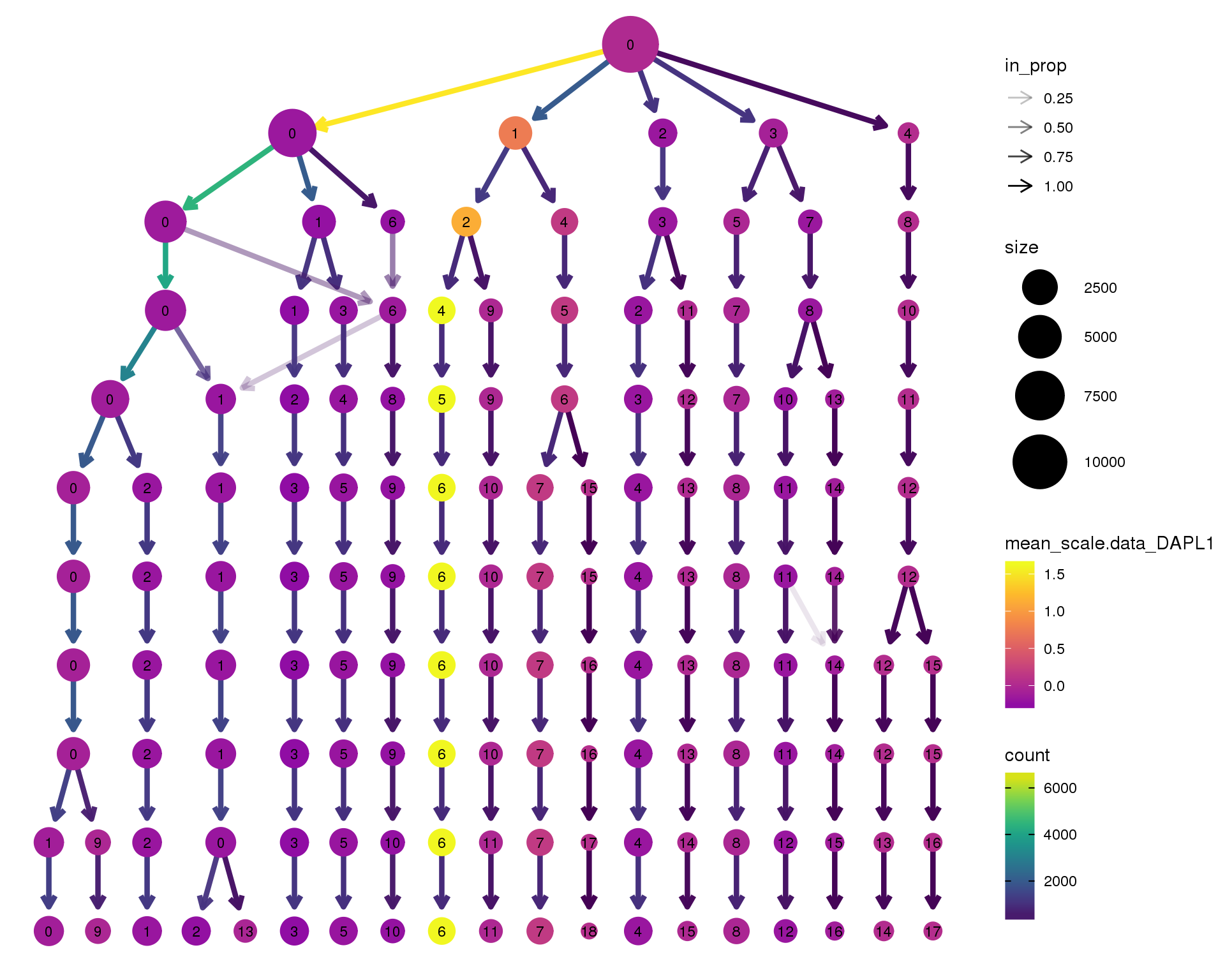
Expand here to see past versions of clustree-DAPL1-1.png:
| Version | Author | Date |
|---|---|---|
| ad10b21 | Luke Zappia | 2018-09-13 |
NPHS1
clustree(combined, node_colour = 'NPHS1',
node_colour_aggr = 'mean',
exprs = 'scale.data') +
scale_colour_viridis_c(option = 'plasma', begin = 0.3)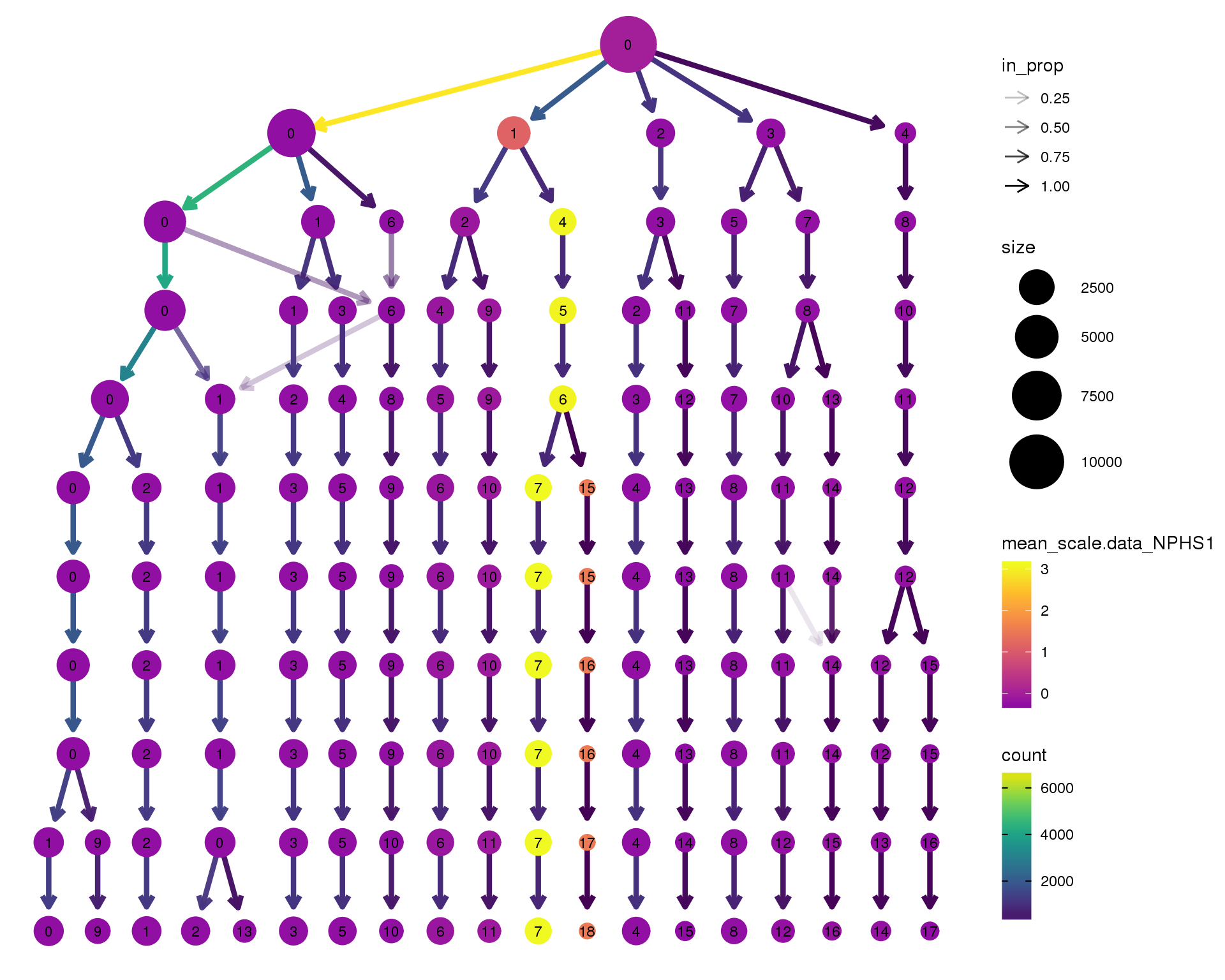
Expand here to see past versions of clustree-NPHS1-1.png:
| Version | Author | Date |
|---|---|---|
| ad10b21 | Luke Zappia | 2018-09-13 |
PODXL
clustree(combined, node_colour = 'PODXL',
node_colour_aggr = 'mean',
exprs = 'scale.data') +
scale_colour_viridis_c(option = 'plasma', begin = 0.3)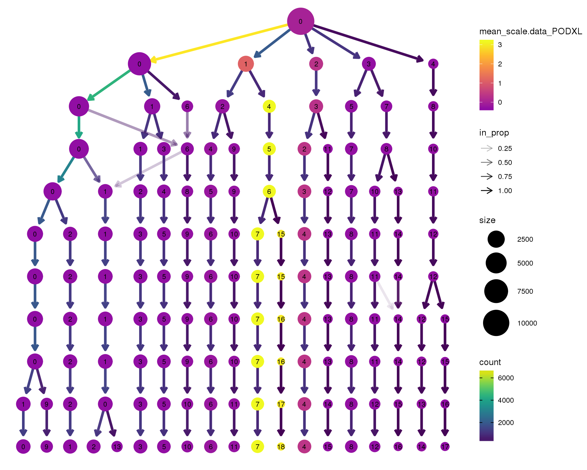
Expand here to see past versions of clustree-PODXL-1.png:
| Version | Author | Date |
|---|---|---|
| ad10b21 | Luke Zappia | 2018-09-13 |
S100A8
clustree(combined, node_colour = 'S100A8',
node_colour_aggr = 'mean',
exprs = 'scale.data') +
scale_colour_viridis_c(option = 'plasma', begin = 0.3)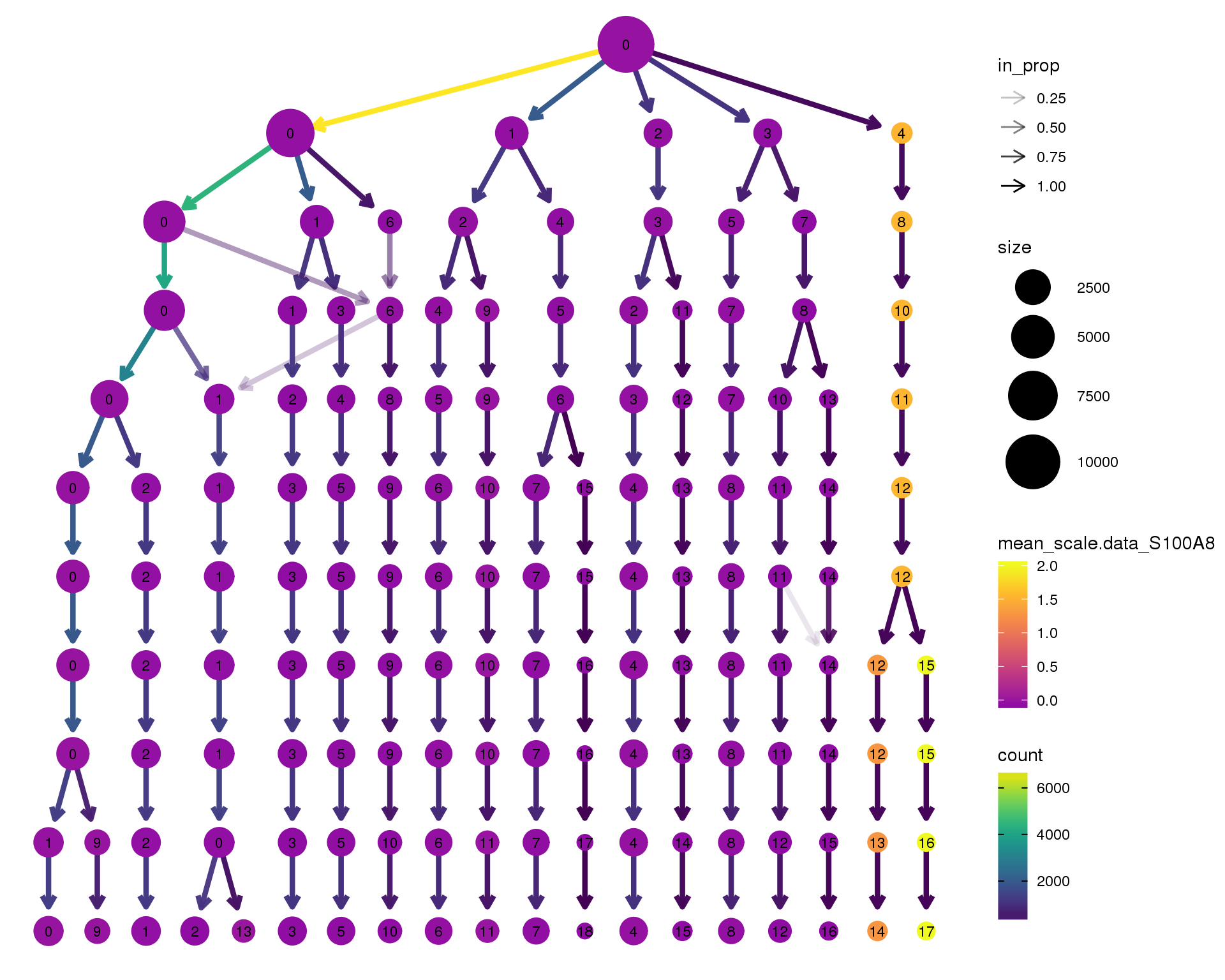
Expand here to see past versions of clustree-S100A8-1.png:
| Version | Author | Date |
|---|---|---|
| ad10b21 | Luke Zappia | 2018-09-13 |
TYROBP
clustree(combined, node_colour = 'TYROBP',
node_colour_aggr = 'mean',
exprs = 'scale.data') +
scale_colour_viridis_c(option = 'plasma', begin = 0.3)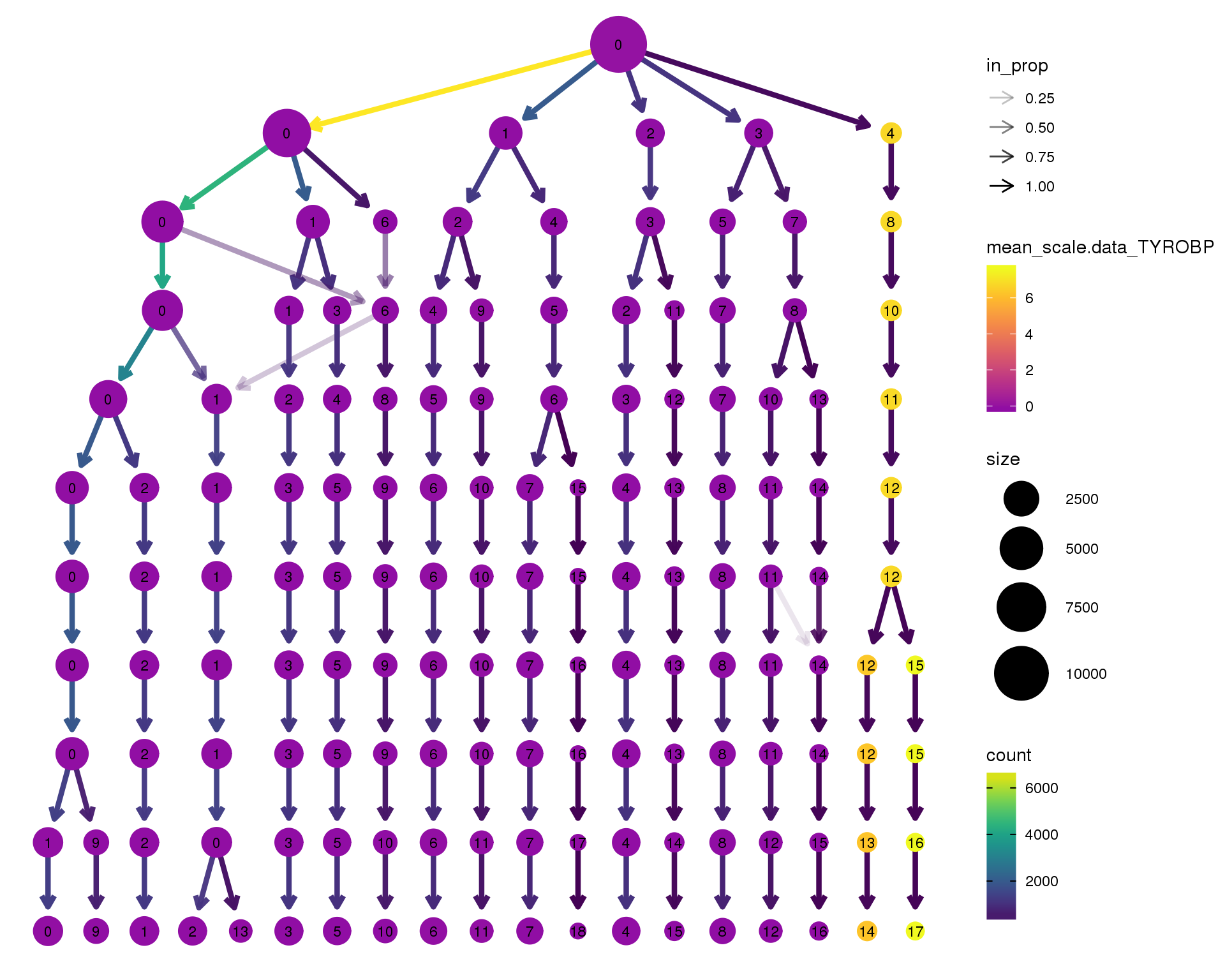
Expand here to see past versions of clustree-TYROBP-1.png:
| Version | Author | Date |
|---|---|---|
| ad10b21 | Luke Zappia | 2018-09-13 |
MAL
clustree(combined, node_colour = 'MAL',
node_colour_aggr = 'mean',
exprs = 'scale.data') +
scale_colour_viridis_c(option = 'plasma', begin = 0.3)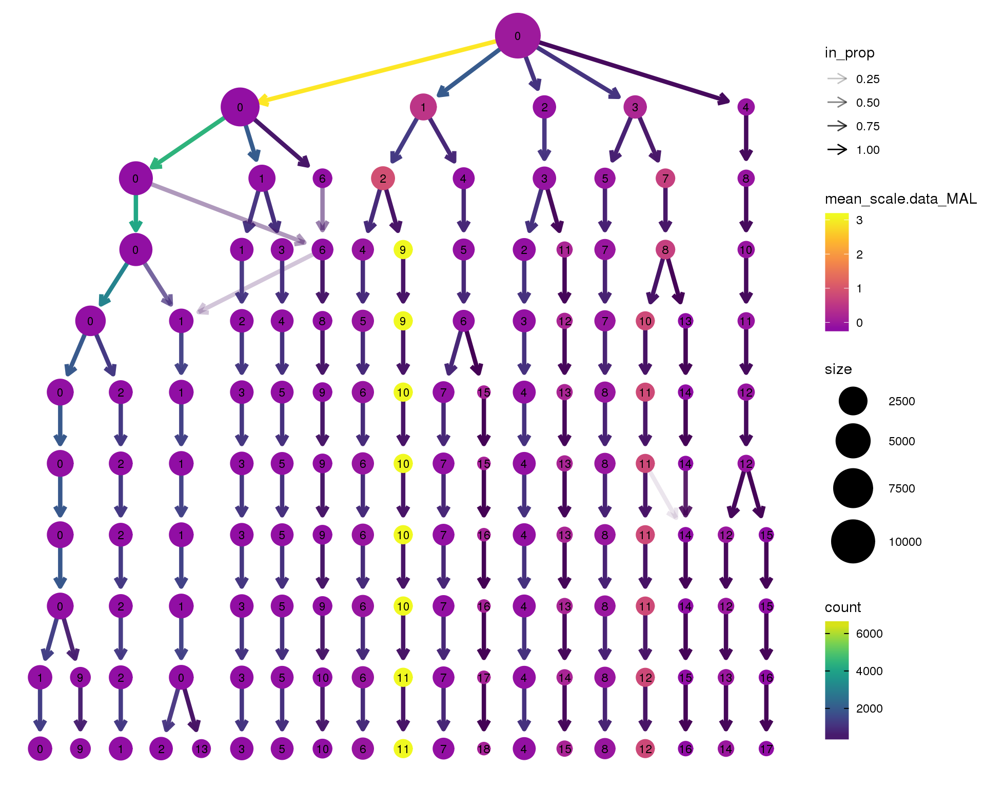
Expand here to see past versions of clustree-MAL-1.png:
| Version | Author | Date |
|---|---|---|
| ad10b21 | Luke Zappia | 2018-09-13 |
EMX2
clustree(combined, node_colour = 'EMX2',
node_colour_aggr = 'mean',
exprs = 'scale.data') +
scale_colour_viridis_c(option = 'plasma', begin = 0.3)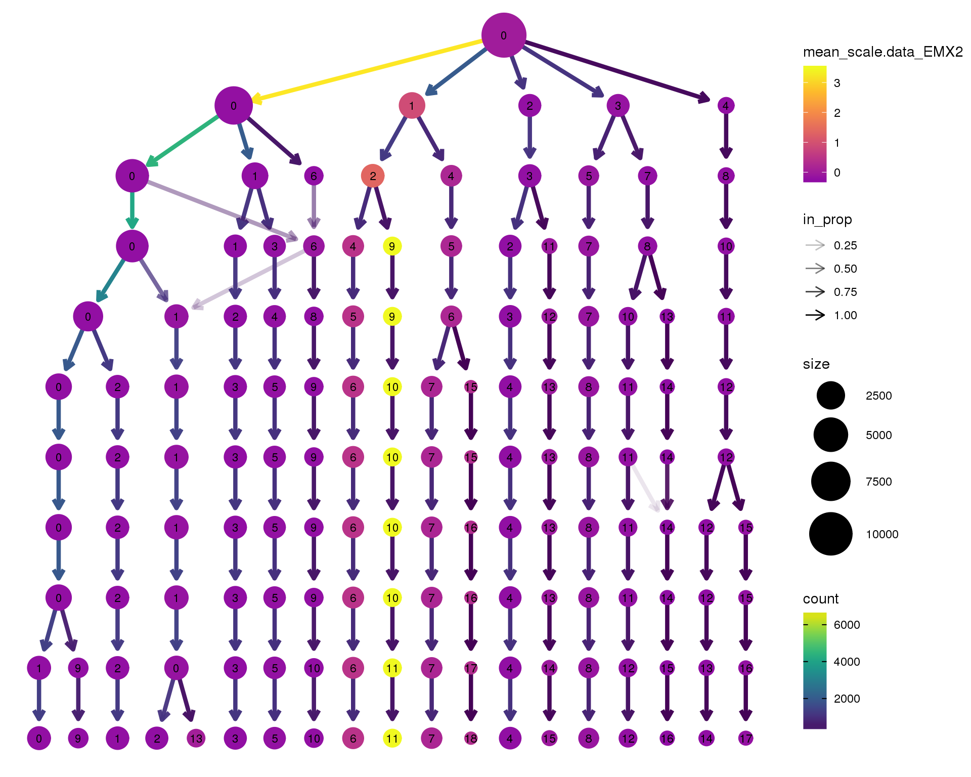
Expand here to see past versions of clustree-EMX2-1.png:
| Version | Author | Date |
|---|---|---|
| ad10b21 | Luke Zappia | 2018-09-13 |
LRP2
clustree(combined, node_colour = 'LRP2',
node_colour_aggr = 'mean',
exprs = 'scale.data') +
scale_colour_viridis_c(option = 'plasma', begin = 0.3)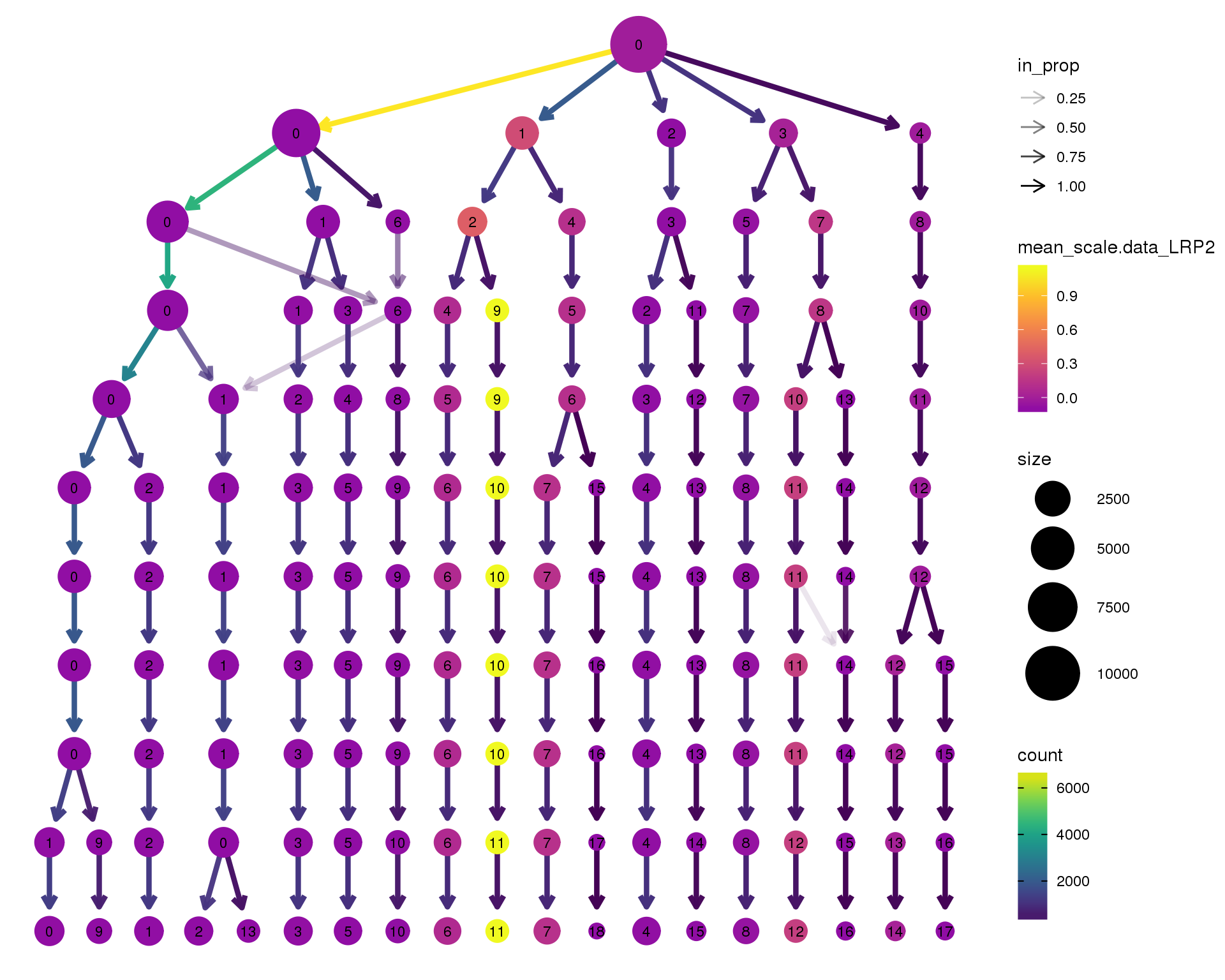
Expand here to see past versions of clustree-LRP2-1.png:
| Version | Author | Date |
|---|---|---|
| ad10b21 | Luke Zappia | 2018-09-13 |
GATA3
clustree(combined, node_colour = 'GATA3',
node_colour_aggr = 'mean',
exprs = 'scale.data') +
scale_colour_viridis_c(option = 'plasma', begin = 0.3)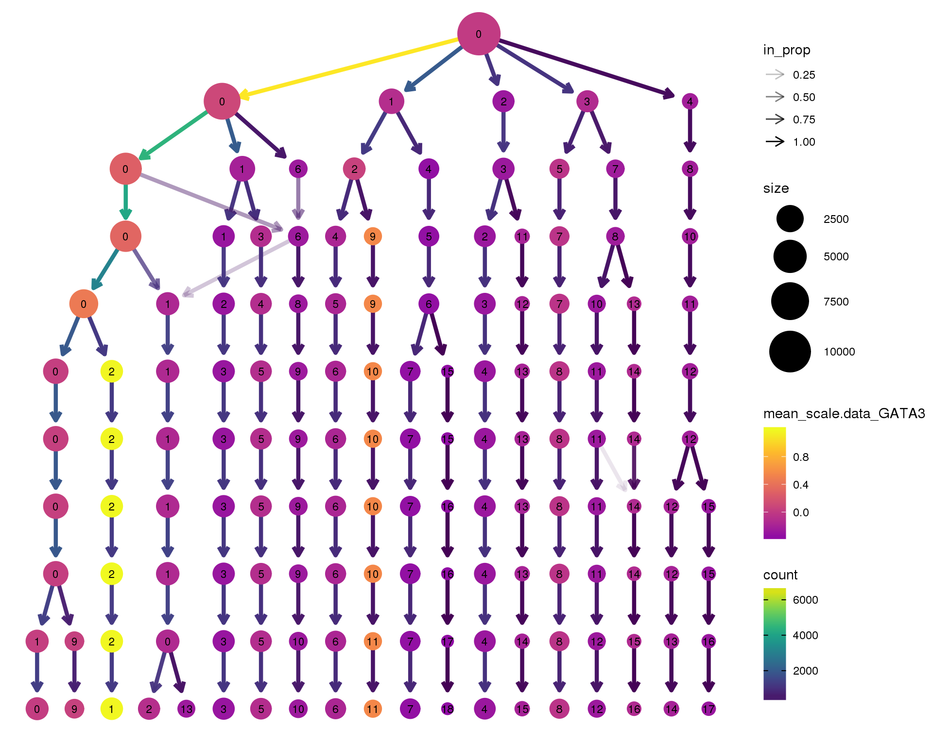
Expand here to see past versions of clustree-GATA3-1.png:
| Version | Author | Date |
|---|---|---|
| ad10b21 | Luke Zappia | 2018-09-13 |
SLC12A1
clustree(combined, node_colour = 'SLC12A1',
node_colour_aggr = 'mean',
exprs = 'scale.data') +
scale_colour_viridis_c(option = 'plasma', begin = 0.3)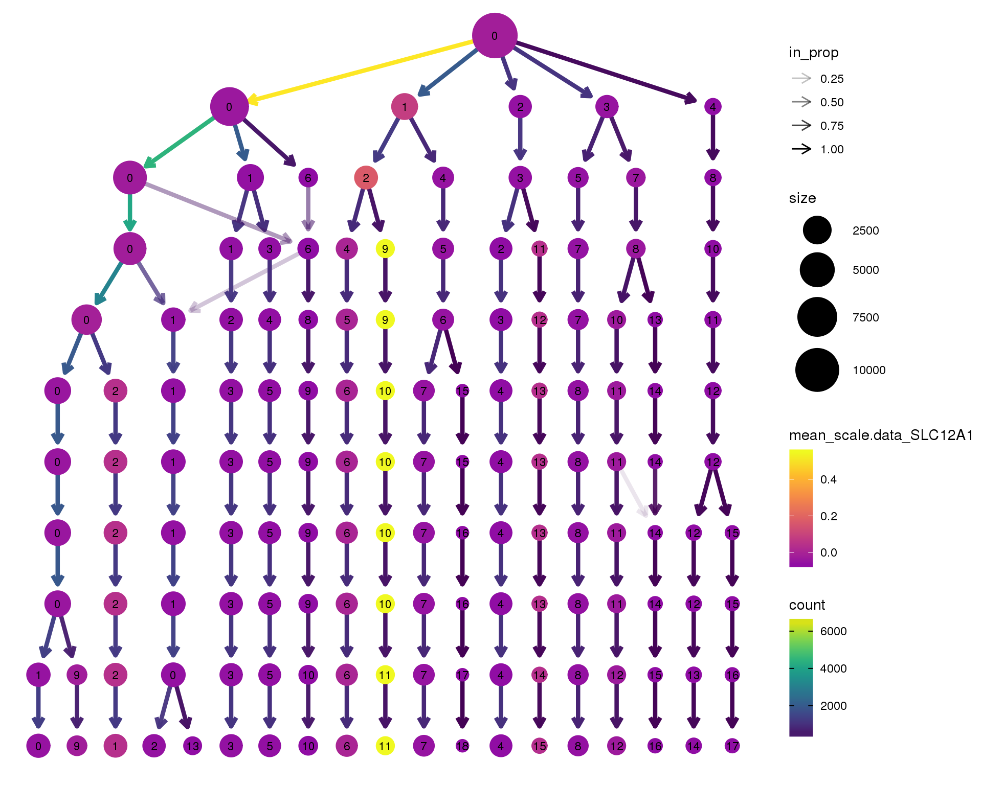
Expand here to see past versions of clustree-SLC12A1-1.png:
| Version | Author | Date |
|---|---|---|
| ad10b21 | Luke Zappia | 2018-09-13 |
SPINT2
clustree(combined, node_colour = 'SPINT2',
node_colour_aggr = 'mean',
exprs = 'scale.data') +
scale_colour_viridis_c(option = 'plasma', begin = 0.3)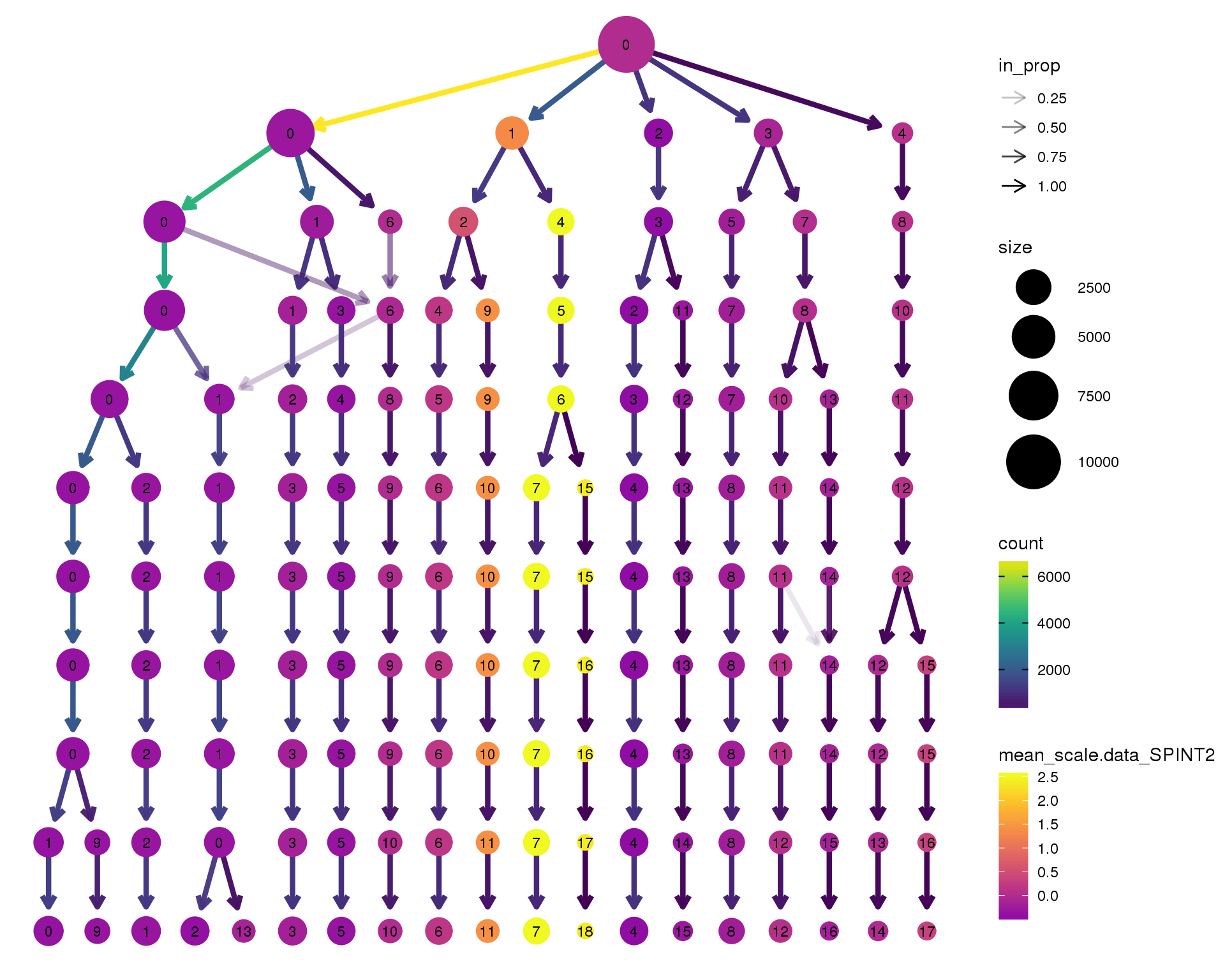
Expand here to see past versions of clustree-SPINT2-1.png:
| Version | Author | Date |
|---|---|---|
| ad10b21 | Luke Zappia | 2018-09-13 |
TUBB2B
clustree(combined, node_colour = 'TUBB2B',
node_colour_aggr = 'mean',
exprs = 'scale.data') +
scale_colour_viridis_c(option = 'plasma', begin = 0.3)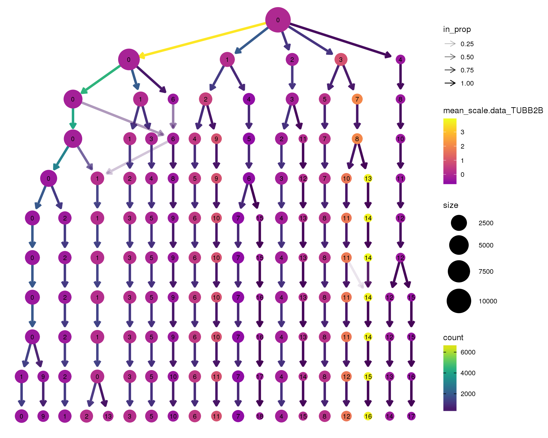
Expand here to see past versions of clustree-TUBB2B-1.png:
| Version | Author | Date |
|---|---|---|
| ad10b21 | Luke Zappia | 2018-09-13 |
STMN2
clustree(combined, node_colour = 'STMN2',
node_colour_aggr = 'mean',
exprs = 'scale.data') +
scale_colour_viridis_c(option = 'plasma', begin = 0.3)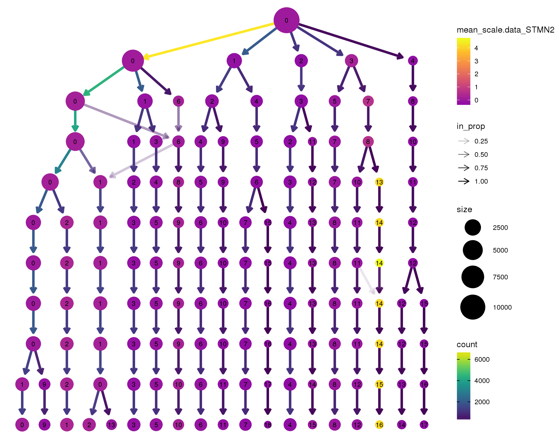
Expand here to see past versions of clustree-STMN2-1.png:
| Version | Author | Date |
|---|---|---|
| ad10b21 | Luke Zappia | 2018-09-13 |
TTYH1
clustree(combined, node_colour = 'TTYH1',
node_colour_aggr = 'mean',
exprs = 'scale.data') +
scale_colour_viridis_c(option = 'plasma', begin = 0.3)
HBA1
clustree(combined, node_colour = 'HBA1',
node_colour_aggr = 'mean',
exprs = 'scale.data') +
scale_colour_viridis_c(option = 'plasma', begin = 0.3)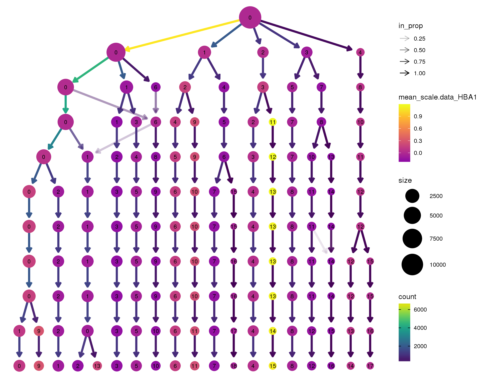
Expand here to see past versions of clustree-HBA1-1.png:
| Version | Author | Date |
|---|---|---|
| ad10b21 | Luke Zappia | 2018-09-13 |
HBG1
clustree(combined, node_colour = 'HBG1',
node_colour_aggr = 'mean',
exprs = 'scale.data') +
scale_colour_viridis_c(option = 'plasma', begin = 0.3)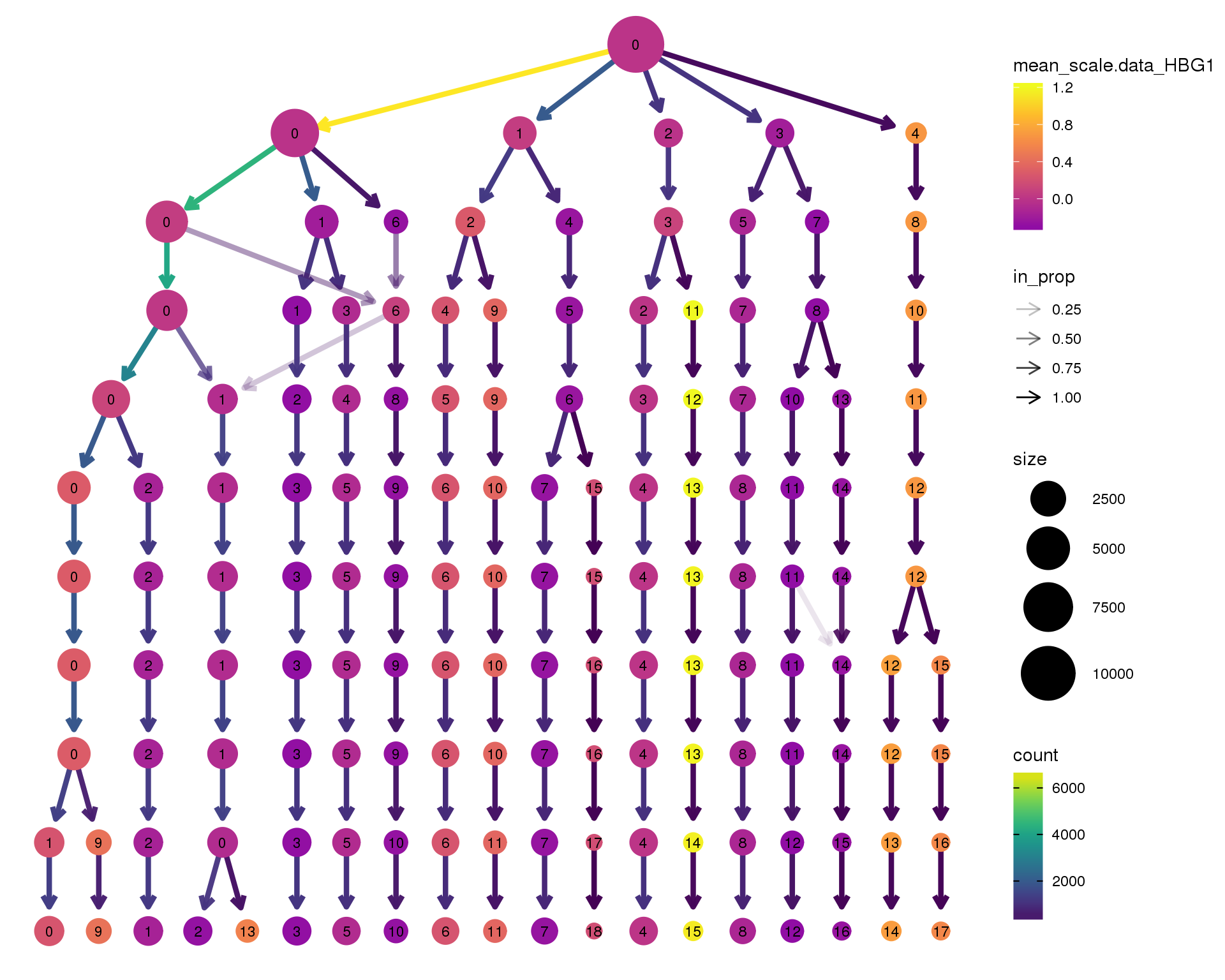
Expand here to see past versions of clustree-HBG1-1.png:
| Version | Author | Date |
|---|---|---|
| ad10b21 | Luke Zappia | 2018-09-13 |
Selected resolution
res <- 0.5
combined <- SetIdent(combined,
ident.use = combined@meta.data[, paste0("res.", res)])
n.clusts <- length(unique(combined@ident))Based on these plots we will use a resolution of 0.5.
Clusters
Let’s have a look at the clusters on a t-SNE plot.
p1 <- TSNEPlot(combined, do.return = TRUE, pt.size = 0.5,
group.by = "DatasetSample")
p2 <- TSNEPlot(combined, do.label = TRUE, do.return = TRUE, pt.size = 0.5)
plot_grid(p1, p2)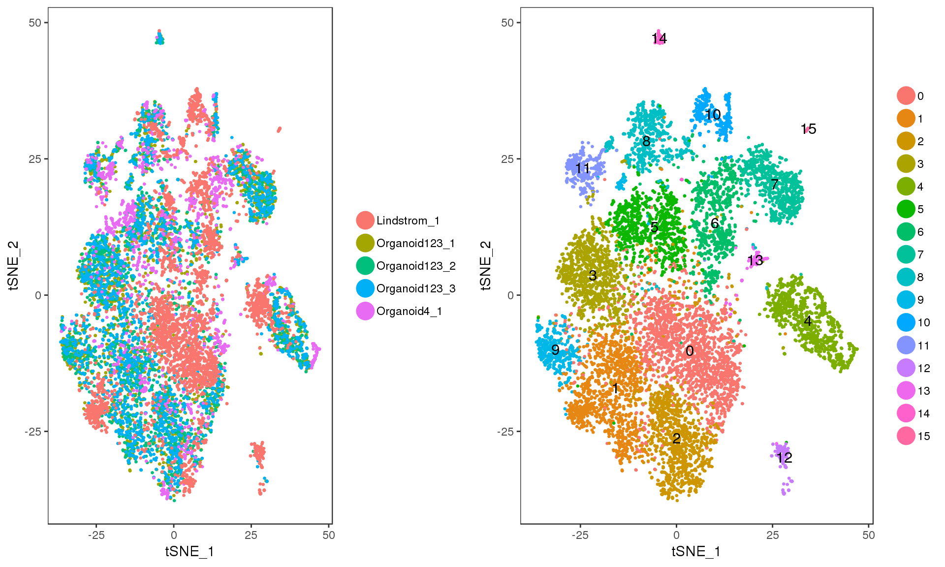
Expand here to see past versions of tSNE-1.png:
| Version | Author | Date |
|---|---|---|
| 5476164 | Luke Zappia | 2018-08-10 |
We can also look at the number of cells in each cluster.
plot.data <- combined@meta.data %>%
select(Dataset, cluster = paste0("res.", res)) %>%
mutate(cluster = factor(as.numeric(cluster))) %>%
group_by(cluster, Dataset) %>%
summarise(count = n()) %>%
mutate(clust_total = sum(count)) %>%
mutate(clust_prop = count / clust_total) %>%
group_by(Dataset) %>%
mutate(dataset_total = sum(count)) %>%
ungroup() %>%
mutate(dataset_prop = count / dataset_total)
ggplot(plot.data, aes(x = cluster, y = count, fill = Dataset)) +
geom_col()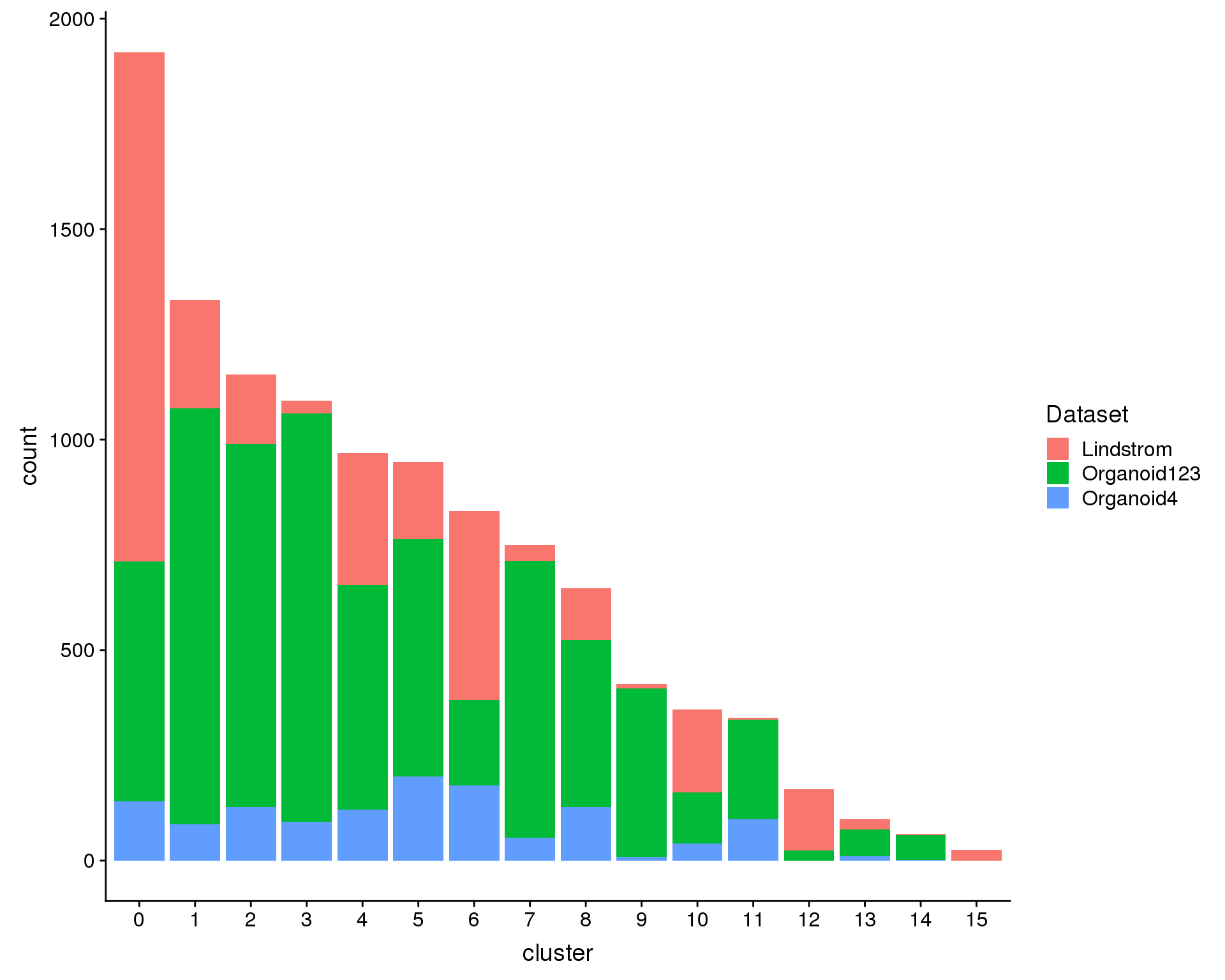
Expand here to see past versions of cluster-sizes-1.png:
| Version | Author | Date |
|---|---|---|
| 5476164 | Luke Zappia | 2018-08-10 |
We are also interested in what proportions of the cells in each cluster come from each datasets (i.e. are there dataset specific clusters?).
ggplot(plot.data, aes(x = cluster, y = clust_prop, fill = Dataset)) +
geom_col()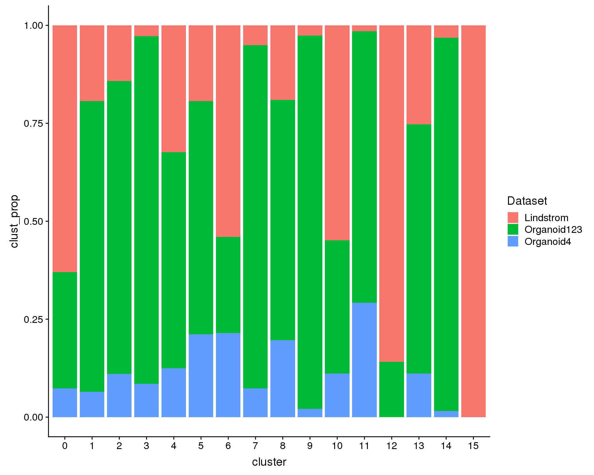
Expand here to see past versions of cluster-props-1.png:
| Version | Author | Date |
|---|---|---|
| 5476164 | Luke Zappia | 2018-08-10 |
Alternatively we can look at what proportion of the cells in each dataset are in each cluster. If each dataset has the same distribution of cell types the heights of the bars should be the same.
ggplot(plot.data, aes(x = cluster, y = dataset_prop, fill = Dataset)) +
geom_col(position = position_dodge(0.9))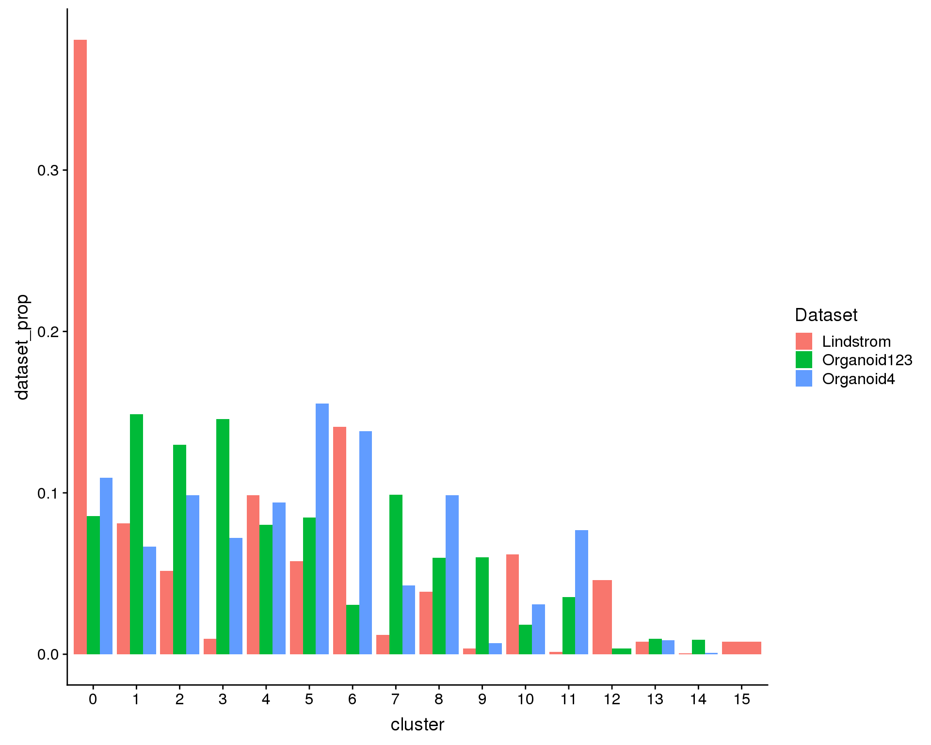
Expand here to see past versions of dataset-props-1.png:
| Version | Author | Date |
|---|---|---|
| 5476164 | Luke Zappia | 2018-08-10 |
Marker genes
Clustering is not very useful if we don’t know what cell types the clusters represent. One way to work that out is to look at marker genes, genes that are differentially expressed in one cluster compared to all other cells. Here we use the Wilcoxon rank sum test genes that are present in at least 10 percent of cells in at least one group (a cluster or all other cells).
markers <- bplapply(seq_len(n.clusts) - 1, function(cl) {
cl.markers <- FindMarkers(combined, cl, logfc.threshold = 0, min.pct = 0.1,
print.bar = FALSE)
cl.markers$cluster <- cl
cl.markers$gene <- rownames(cl.markers)
return(cl.markers)
}, BPPARAM = bpparam)
markers <- bind_rows(markers) %>%
select(gene, cluster, everything())Here we print out the top two markers for each cluster.
markers %>% group_by(cluster) %>% top_n(2, abs(avg_logFC)) %>% data.frameA heatmap can give us a better view. We show the top five positive marker genes for each cluster.
top <- markers %>% group_by(cluster) %>% top_n(5, avg_logFC)
cols <- viridis(100)[c(1, 50, 100)]
DoHeatmap(combined, genes.use = top$gene, slim.col.label = TRUE,
remove.key = TRUE, col.low = cols[1], col.mid = cols[2],
col.high = cols[3])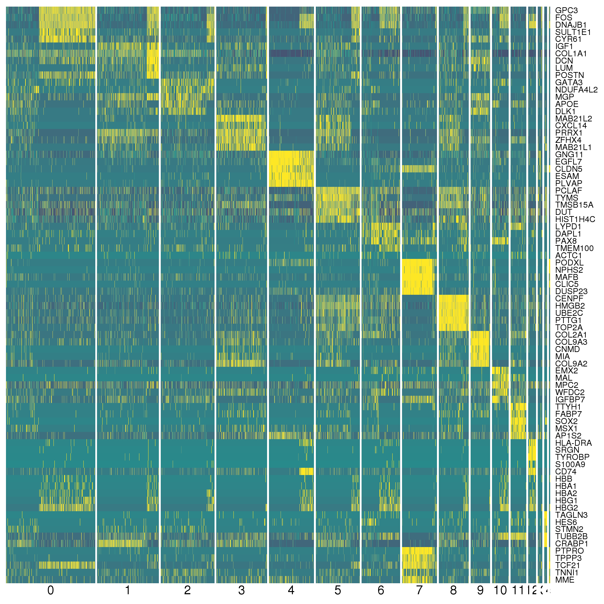
Expand here to see past versions of markers-heatmap-1.png:
| Version | Author | Date |
|---|---|---|
| 5476164 | Luke Zappia | 2018-08-10 |
By cluster
markers.list <- lapply(0:(n.clusts - 1), function(x) {
markers %>%
filter(cluster == x, p_val < 0.05) %>%
dplyr::arrange(-avg_logFC) %>%
select(Gene = gene, LogFC = avg_logFC, pVal = p_val)
})
names(markers.list) <- paste("Cluster", 0:(n.clusts - 1))marker.summary <- markers.list %>%
map2_df(names(markers.list), ~ mutate(.x, Cluster = .y)) %>%
mutate(IsUp = LogFC > 0) %>%
group_by(Cluster) %>%
summarise(Up = sum(IsUp), Down = sum(!IsUp)) %>%
mutate(Down = -Down) %>%
gather(key = "Direction", value = "Count", -Cluster) %>%
mutate(Cluster = factor(Cluster, levels = names(markers.list)))
ggplot(marker.summary,
aes(x = fct_rev(Cluster), y = Count, fill = Direction)) +
geom_col() +
geom_text(aes(y = Count + sign(Count) * max(abs(Count)) * 0.07,
label = abs(Count)),
size = 6, colour = "grey25") +
coord_flip() +
scale_fill_manual(values = c("#377eb8", "#e41a1c")) +
ggtitle("Number of identified genes") +
theme(axis.title = element_blank(),
axis.line = element_blank(),
axis.ticks = element_blank(),
axis.text.x = element_blank(),
legend.position = "bottom")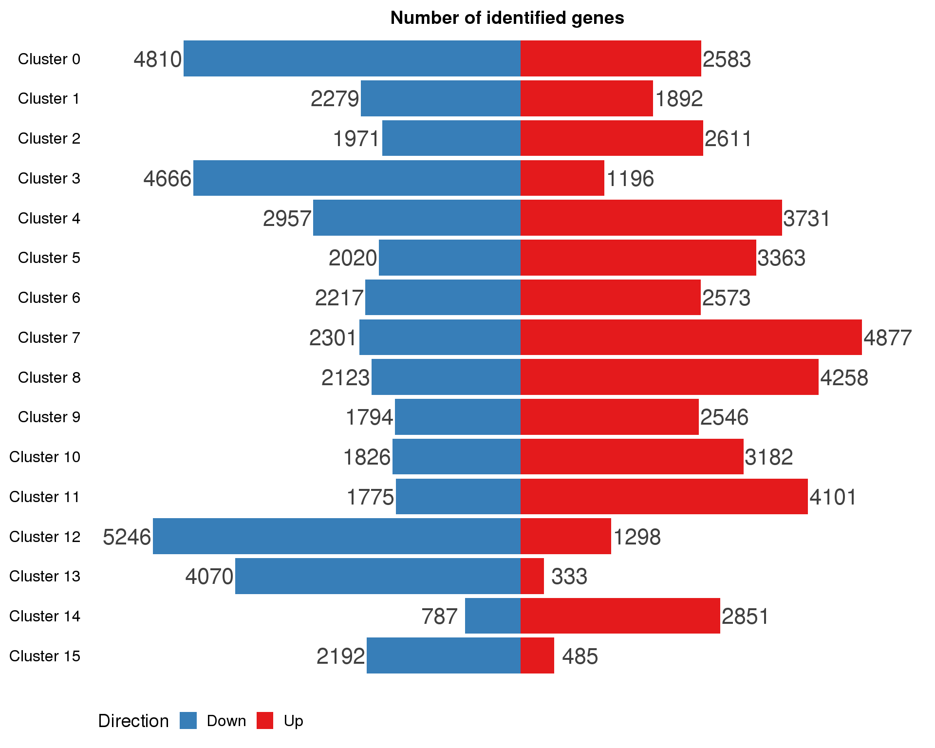
Expand here to see past versions of marker-cluster-counts-1.png:
| Version | Author | Date |
|---|---|---|
| ad10b21 | Luke Zappia | 2018-09-13 |
We can also look at the full table of significant marker genes for each cluster.
src_list <- lapply(0:(n.clusts - 1), function(i) {
src <- c("### {{i}} {.unnumbered}",
"```{r marker-cluster-{{i}}}",
"markers.list[[{{i}} + 1]]",
"```",
"")
knit_expand(text = src)
})
out <- knit_child(text = unlist(src_list),
options = list(echo = FALSE, cache = FALSE))0
1
2
3
4
5
6
7
8
9
10
11
12
13
14
15
Conserved markers
Here we are going to look for genes that are cluster markers in both the Organoid and Lindstrom datasets. Each dataset will be tested individually and the results combined to see if they are present in both datasets.
combined@meta.data$Group <- gsub("[0-9]", "", combined@meta.data$Dataset)
skip <- combined@meta.data %>%
count(Group, Cluster = !! rlang::sym(paste0("res.", res))) %>%
spread(Group, n) %>%
replace_na(list(Organoid = 0L, Lindstrom = 0L)) %>%
rowwise() %>%
mutate(Skip = min(Organoid, Lindstrom) < 3) %>%
arrange(as.numeric(Cluster)) %>%
pull(Skip)Skipped clusters
Testing conserved markers isn’t possible for clusters that only contain cells from one dataset. In this case the following clusters are skipped: 14 and 15
con.markers <- bplapply(seq_len(n.clusts) - 1, function(cl) {
if (skip[cl + 1]) {
message("Skipping cluster ", cl)
cl.markers <- c()
} else {
cl.markers <- FindConservedMarkers(combined, cl, grouping.var = "Group",
logfc.threshold = 0, min.pct = 0.1,
print.bar = FALSE)
cl.markers$cluster <- cl
cl.markers$gene <- rownames(cl.markers)
}
return(cl.markers)
}, BPPARAM = bpparam)
con.markers <- bind_rows(con.markers) %>%
mutate(mean_avg_logFC = rowMeans(select(., ends_with("avg_logFC")))) %>%
select(gene, cluster, mean_avg_logFC, max_pval, minimump_p_val,
everything())Here we print out the top two conserved markers for each cluster.
con.markers %>%
group_by(cluster) %>%
top_n(2, abs(mean_avg_logFC)) %>%
data.frameAgain a heatmap can give us a better view. We show the top five positive conserved marker genes for each cluster.
top <- con.markers %>% group_by(cluster) %>% top_n(5, mean_avg_logFC)
cols <- viridis(100)[c(1, 50, 100)]
DoHeatmap(combined, genes.use = top$gene, slim.col.label = TRUE,
remove.key = TRUE, col.low = cols[1], col.mid = cols[2],
col.high = cols[3])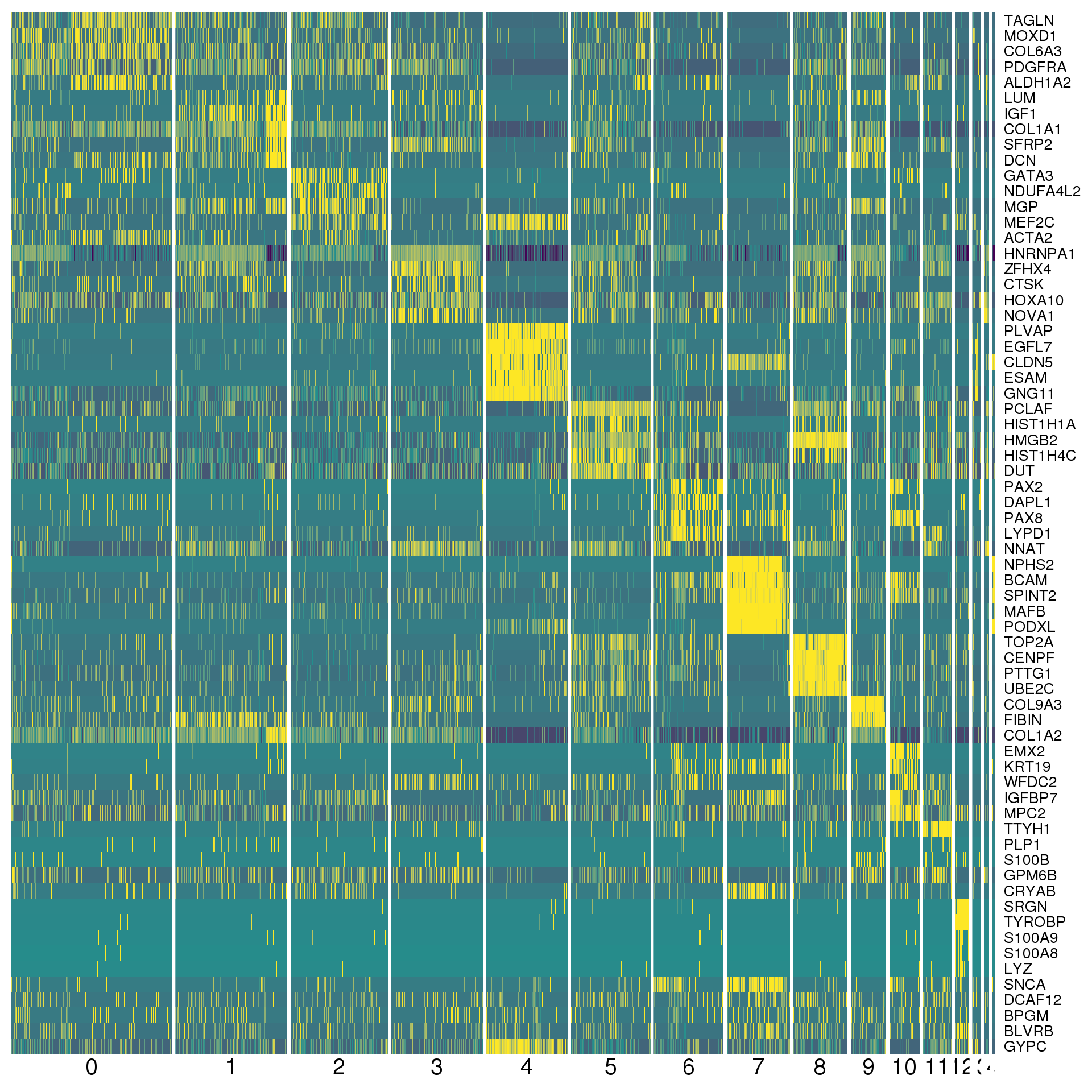
Expand here to see past versions of con-markers-heatmap-1.png:
| Version | Author | Date |
|---|---|---|
| 5476164 | Luke Zappia | 2018-08-10 |
By cluster
con.markers.list <- lapply(0:(n.clusts - 1), function(x) {
con.markers %>%
filter(cluster == x, max_pval < 0.05) %>%
dplyr::arrange(-mean_avg_logFC) %>%
select(Gene = gene,
MeanLogFC= mean_avg_logFC,
MaxPVal = max_pval,
MinPVal = minimump_p_val,
OrganoidLogFC = Organoid_avg_logFC,
OrganoidPVal = Organoid_p_val,
LindstromLogFC = Lindstrom_avg_logFC,
LindstromPVal = Lindstrom_p_val)
})
names(con.markers.list) <- paste("Cluster", 0:(n.clusts - 1))con.marker.summary <- con.markers.list %>%
map2_df(names(con.markers.list), ~ mutate(.x, Cluster = .y)) %>%
mutate(IsUp = MeanLogFC > 0) %>%
group_by(Cluster) %>%
summarise(Up = sum(IsUp), Down = sum(!IsUp)) %>%
mutate(Down = -Down) %>%
gather(key = "Direction", value = "Count", -Cluster) %>%
mutate(Cluster = factor(Cluster, levels = names(markers.list)))
ggplot(con.marker.summary,
aes(x = fct_rev(Cluster), y = Count, fill = Direction)) +
geom_col() +
geom_text(aes(y = Count + sign(Count) * max(abs(Count)) * 0.07,
label = abs(Count)),
size = 6, colour = "grey25") +
coord_flip() +
scale_fill_manual(values = c("#377eb8", "#e41a1c")) +
ggtitle("Number of identified genes") +
theme(axis.title = element_blank(),
axis.line = element_blank(),
axis.ticks = element_blank(),
axis.text.x = element_blank(),
legend.position = "bottom")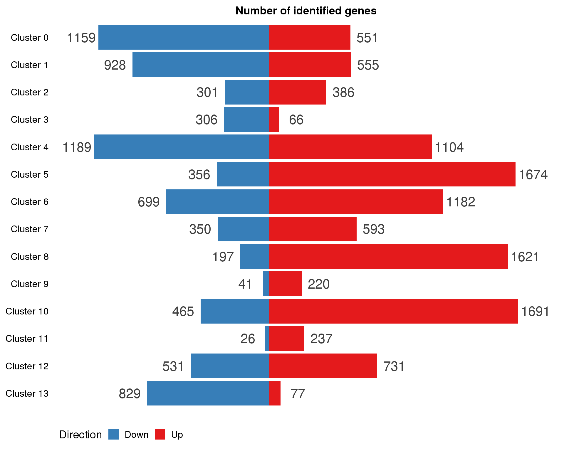
Expand here to see past versions of con-marker-cluster-counts-1.png:
| Version | Author | Date |
|---|---|---|
| ad10b21 | Luke Zappia | 2018-09-13 |
We can also look at the full table of significant conserved marker genes for each cluster.
src_list <- lapply(0:(length(con.markers.list)-1), function(i) {
src <- c("### {{i}} {.unnumbered}",
"```{r con-marker-cluster-{{i}}}",
"con.markers.list[[{{i}} + 1]]",
"```",
"")
knit_expand(text = src)
})
out <- knit_child(text = unlist(src_list),
options = list(echo = FALSE, cache = FALSE))0
1
2
3
4
5
6
7
8
9
10
11
12
13
14
15
Within cluster DE
We can also look for genes that are differentially expressed between the two datasets in the same cluster. This might help to identify differences in the same cell type between the difference experiments.
combined@meta.data$GroupCluster <- paste(combined@meta.data$Group,
combined@ident, sep = "_")
combined <- StashIdent(combined, save.name = "Cluster")
combined <- SetAllIdent(combined, id = "GroupCluster")plot.data <- AverageExpression(combined, show.progress = FALSE) %>%
rownames_to_column("Gene") %>%
gather(key = "GroupCluster", value = "AvgExp", -Gene) %>%
separate(GroupCluster, c("Group", "Cluster"), sep = "_") %>%
mutate(Cluster = factor(as.numeric(Cluster))) %>%
mutate(LogAvgExp = log1p(AvgExp)) %>%
select(-AvgExp) %>%
spread(Group, LogAvgExp) %>%
replace_na(list(Organoid = 0, Lindstrom = 0)) %>%
mutate(Avg = 0.5 * (Organoid + Lindstrom),
Diff = Organoid - Lindstrom)
ggplot(plot.data, aes(x = Avg, y = Diff)) +
geom_hline(yintercept = 0, colour = "red") +
geom_point(size = 0.6, alpha = 0.2) +
xlab("0.5 * (Organoid + Lindstrom)") +
ylab("Organoid - Lindstrom") +
facet_wrap(~ Cluster)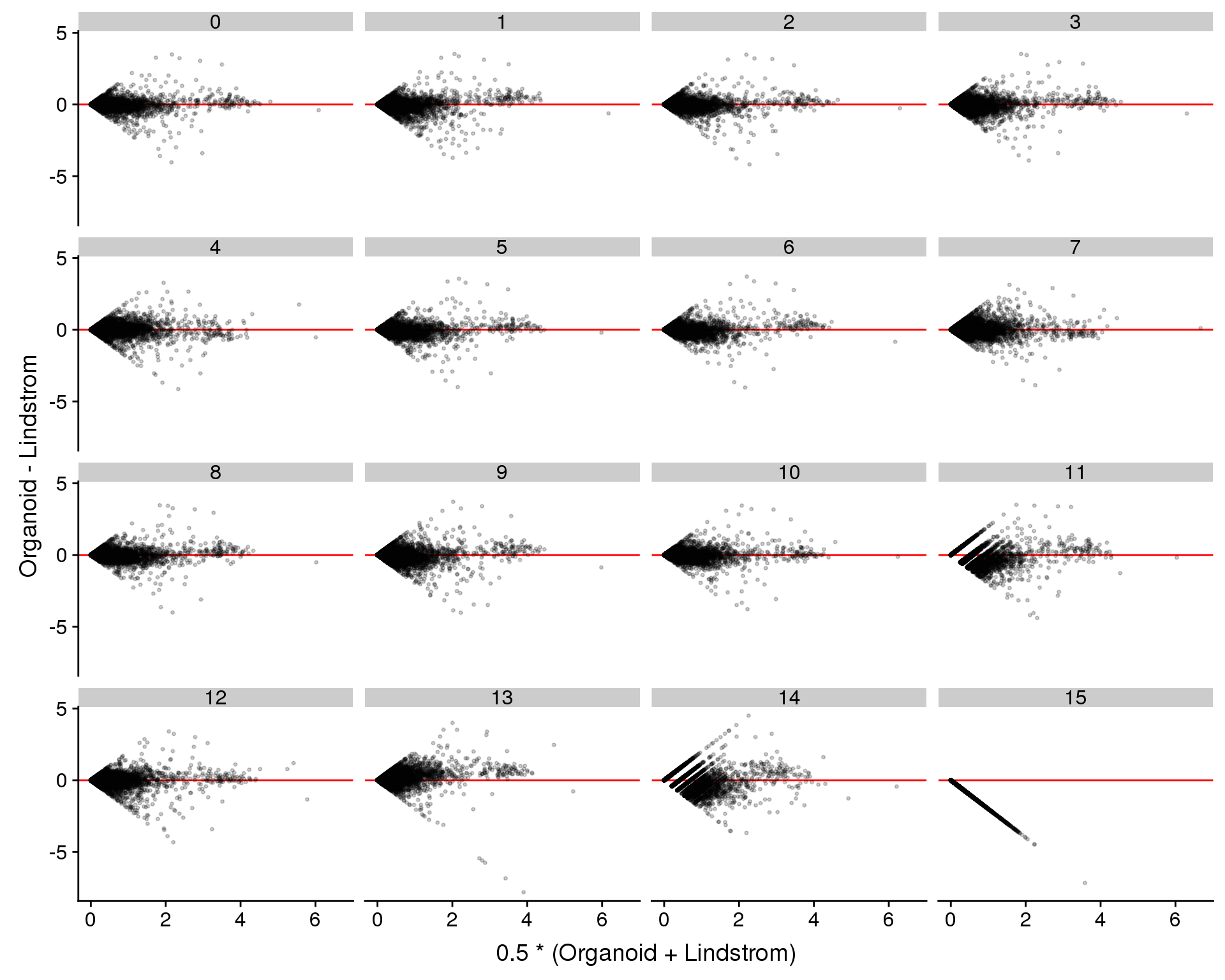
Expand here to see past versions of de-plots-1.png:
| Version | Author | Date |
|---|---|---|
| 5476164 | Luke Zappia | 2018-08-10 |
cluster.de <- bplapply(seq_len(n.clusts) - 1, function(cl) {
if (skip[cl + 1]) {
message("Skipping cluster ", cl)
cl.de <- c()
} else {
cl.de <- FindMarkers(combined, paste("Organoid", cl, sep = "_"),
paste("Lindstrom", cl, sep = "_"),
logfc.threshold = 0, min.pct = 0.1,
print.bar = FALSE)
cl.de$cluster <- cl
cl.de$gene <- rownames(cl.de)
}
return(cl.de)
}, BPPARAM = bpparam)
cluster.de <- bind_rows(cluster.de) %>%
select(gene, cluster, everything())Here we print out the top two DE genes for each cluster.
cluster.de %>% group_by(cluster) %>% top_n(2, abs(avg_logFC)) %>% data.frameAgain a heatmap can give us a better view. We show the top five positive DE genes for each cluster.
top <- cluster.de %>% group_by(cluster) %>% top_n(5, avg_logFC)
cols <- viridis(100)[c(1, 50, 100)]
DoHeatmap(combined, genes.use = top$gene, slim.col.label = TRUE,
remove.key = TRUE, col.low = cols[1], col.mid = cols[2],
col.high = cols[3])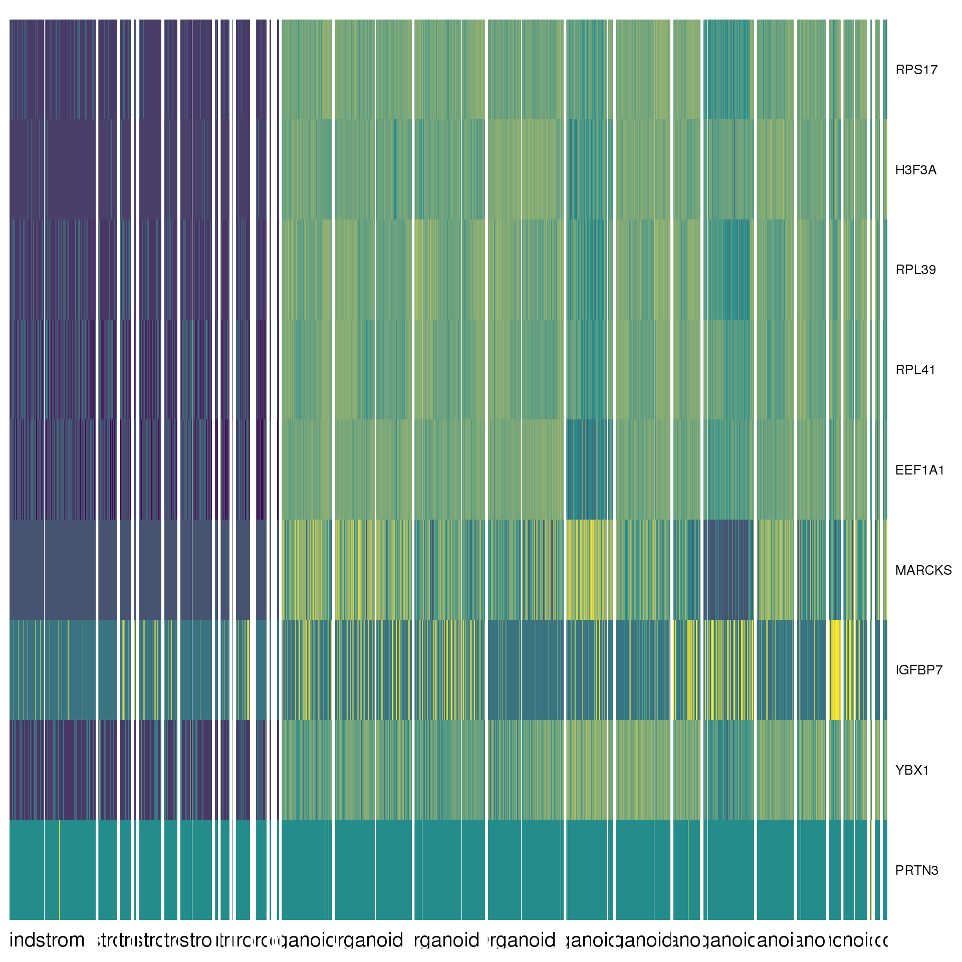
Expand here to see past versions of de-heatmap-1.png:
| Version | Author | Date |
|---|---|---|
| 5476164 | Luke Zappia | 2018-08-10 |
By cluster
cluster.de.list <- lapply(0:(n.clusts - 1), function(x) {
cluster.de %>%
filter(cluster == x, p_val < 0.05) %>%
dplyr::arrange(p_val) %>%
select(Gene = gene, LogFC = avg_logFC, pVal = p_val)
})
names(cluster.de.list) <- paste("Cluster", 0:(n.clusts - 1))cluster.de.summary <- cluster.de.list %>%
map2_df(names(cluster.de.list), ~ mutate(.x, Cluster = .y)) %>%
mutate(IsUp = LogFC > 0) %>%
group_by(Cluster) %>%
summarise(Up = sum(IsUp), Down = sum(!IsUp)) %>%
mutate(Down = -Down) %>%
gather(key = "Direction", value = "Count", -Cluster) %>%
mutate(Cluster = factor(Cluster, levels = names(markers.list)))
ggplot(cluster.de.summary,
aes(x = fct_rev(Cluster), y = Count, fill = Direction)) +
geom_col() +
geom_text(aes(y = Count + sign(Count) * max(abs(Count)) * 0.07,
label = abs(Count)),
size = 6, colour = "grey25") +
coord_flip() +
scale_fill_manual(values = c("#377eb8", "#e41a1c")) +
ggtitle("Number of identified genes") +
theme(axis.title = element_blank(),
axis.line = element_blank(),
axis.ticks = element_blank(),
axis.text.x = element_blank(),
legend.position = "bottom")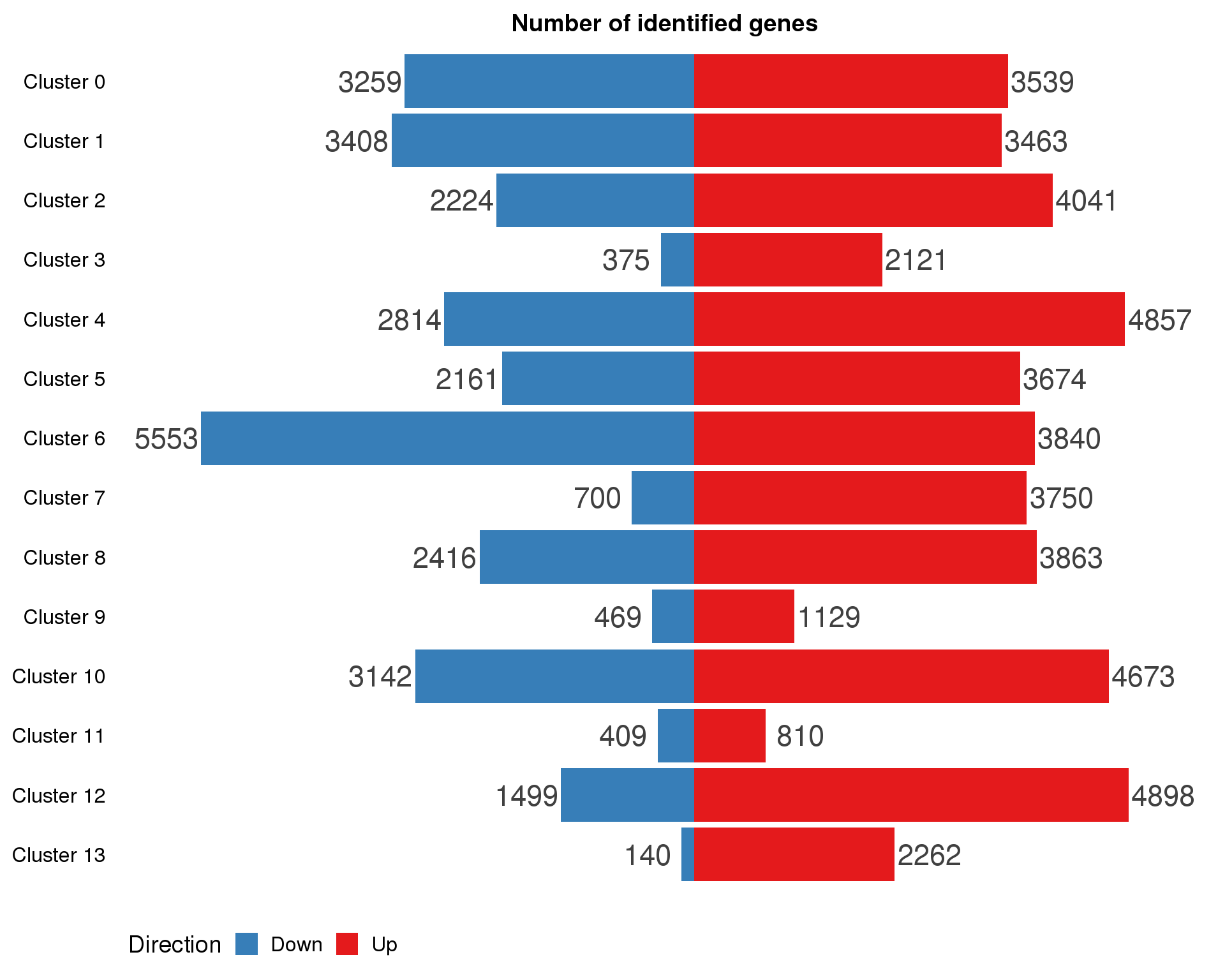
Expand here to see past versions of de-cluster-counts-1.png:
| Version | Author | Date |
|---|---|---|
| ad10b21 | Luke Zappia | 2018-09-13 |
We can also look at the full table of significant DE genes for each cluster.
src_list <- lapply(0:(length(cluster.de.list) - 1), function(i) {
src <- c("### {{i}} {.unnumbered}",
"```{r de-cluster-{{i}}}",
"cluster.de.list[[{{i}} + 1]]",
"```",
"")
knit_expand(text = src)
})
out <- knit_child(text = unlist(src_list),
options = list(echo = FALSE, cache = FALSE))0
1
2
3
4
5
6
7
8
9
10
11
12
13
14
15
Traditional DE
To see if there are any global differences between the datasets we are going to perform traditional differential expression testing between the two groups.
combined <- SetAllIdent(combined, id = "Group")de <- FindMarkers(combined, "Organoid", "Lindstrom", logfc.threshold = 0,
min.pct = 0.1, print.bar = FALSE)de <- de %>% rownames_to_column("gene")
de %>% top_n(10, avg_logFC) %>% data.framecombined <- SetAllIdent(combined, id = "Cluster")From these results we can identify an overall signature of the differences between the datasets by selecting significant genes with an absolute log foldchange greater than 0.5.
de.sig <- de %>%
filter(p_val_adj < 0.05, abs(avg_logFC) > 0.5) %>%
pull(gene)This identifies a signature with 374 genes.
This signature can then be removed from the within cluster differential expression results to better highlight biological differences.
cluster.de.filt <- filter(cluster.de, !(gene %in% de.sig))
cluster.de.list.filt <- map(cluster.de.list,
function(x) {filter(x, !(Gene %in% de.sig))})Gene plots
Plots of known kidney genes we are specifically interested in.
SplitDotPlotGG(combined, grouping.var = "Group",
genes.plot = c("ZEB2", "PDGFRA", "PDGFRB", "MFAP4", "KCNE4",
"TCF12", "REN", "DLK1", "GATA3", "TCF21",
"PRRX1", "DCN", "PECAM1", "CDH5", "KDR", "PAX2",
"LYPD1", "DAPL1", "PODXL", "NPHS2", "MAFB",
"HMGB2", "CENPU", "SFRP2", "NFIA", "ASPN",
"CENPA", "IGFBP7", "EMX2", "MAL"),
cols.use = c("#E41A1C", "#377EB8"),
x.lab.rot = TRUE)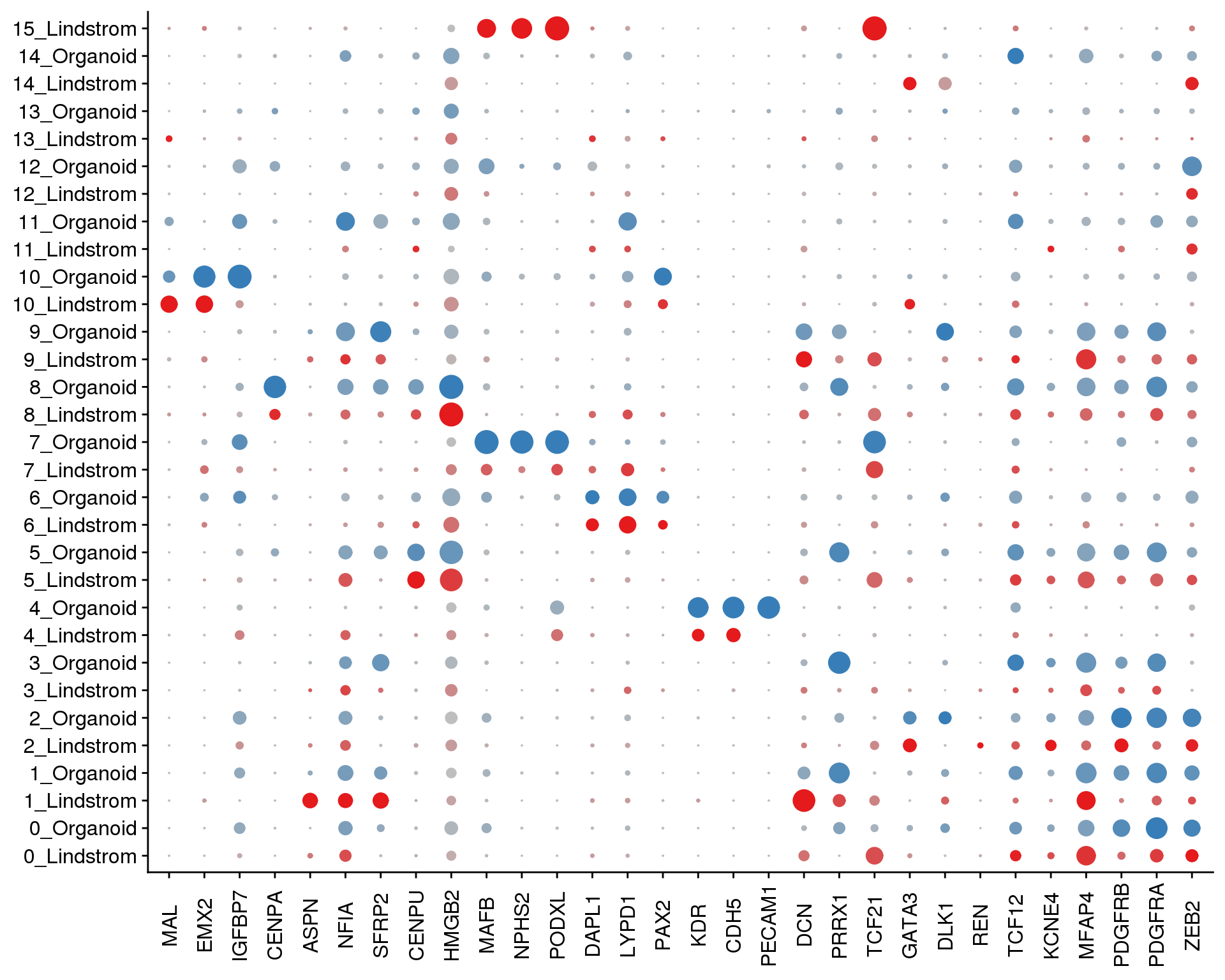
Expand here to see past versions of split-dotplot-1.png:
| Version | Author | Date |
|---|---|---|
| 5476164 | Luke Zappia | 2018-08-10 |
SplitDotPlotGG(combined, grouping.var = "Group",
genes.plot = c("SULT1E1", "ACTA2", "TAGLN", "MAB21L2", "CXCL14",
"PRRX1", "REN", "DLK1", "GATA3", "CRABP1",
"FIBIN", "OGN", "PECAM1", "CDH5", "KDR", "LYPD1",
"DAPL1", "TMEM100", "PODXL", "NPHS2", "MAFB",
"HIST1H1A", "HMGB2", "CENPU", "DCN", "LUM",
"SFRP2", "IGFBP7", "EMX2", "MAL", "TTYH1",
"FABP7", "TUBB2B", "TYROBP", "LYZ", "S100A9",
"STMN2", "ATOH1", "HBG2", "HBG1",
"HBB"),
cols.use = c("#E41A1C", "#377EB8"),
x.lab.rot = TRUE)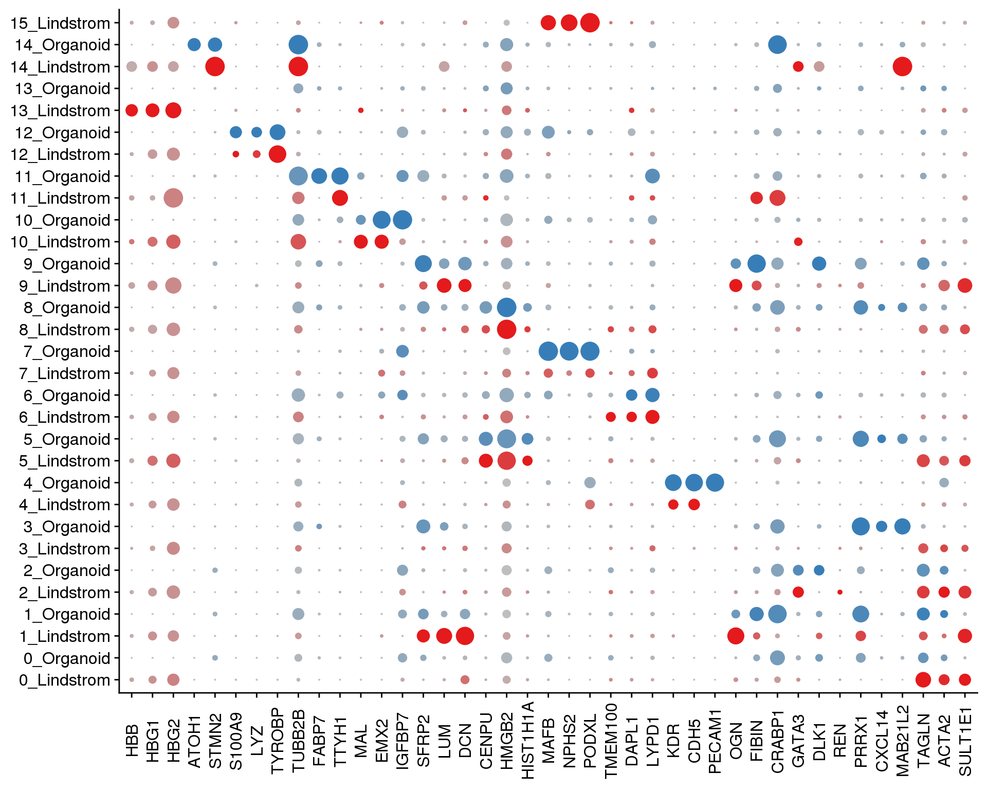
Expand here to see past versions of split-dotplot2-1.png:
| Version | Author | Date |
|---|---|---|
| 5476164 | Luke Zappia | 2018-08-10 |
SplitDotPlotGG(combined, grouping.var = "Group",
genes.plot = c("HSPA1A", "DNAJB1", "FOS", "H3F3A", "EEF1A1",
"MARCKS"),
cols.use = c("#E41A1C", "#377EB8"),
x.lab.rot = TRUE)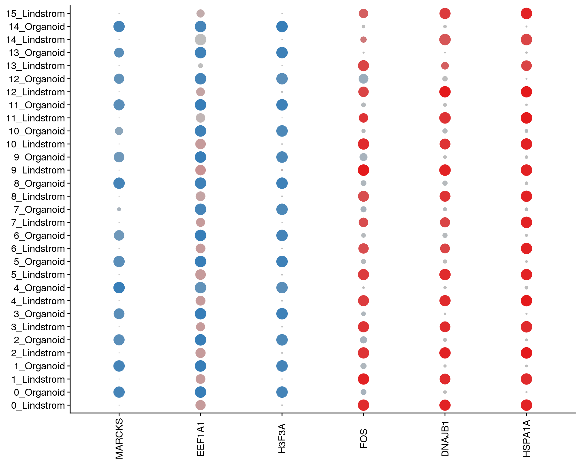
Expand here to see past versions of split-dotplot3-1.png:
| Version | Author | Date |
|---|---|---|
| 5476164 | Luke Zappia | 2018-08-10 |
FeaturePlot(combined, c("HSPA1A", "DNAJB1", "FOS", "H3F3A", "EEF1A1", "MARCKS"),
cols.use = viridis(100), no.axes = TRUE)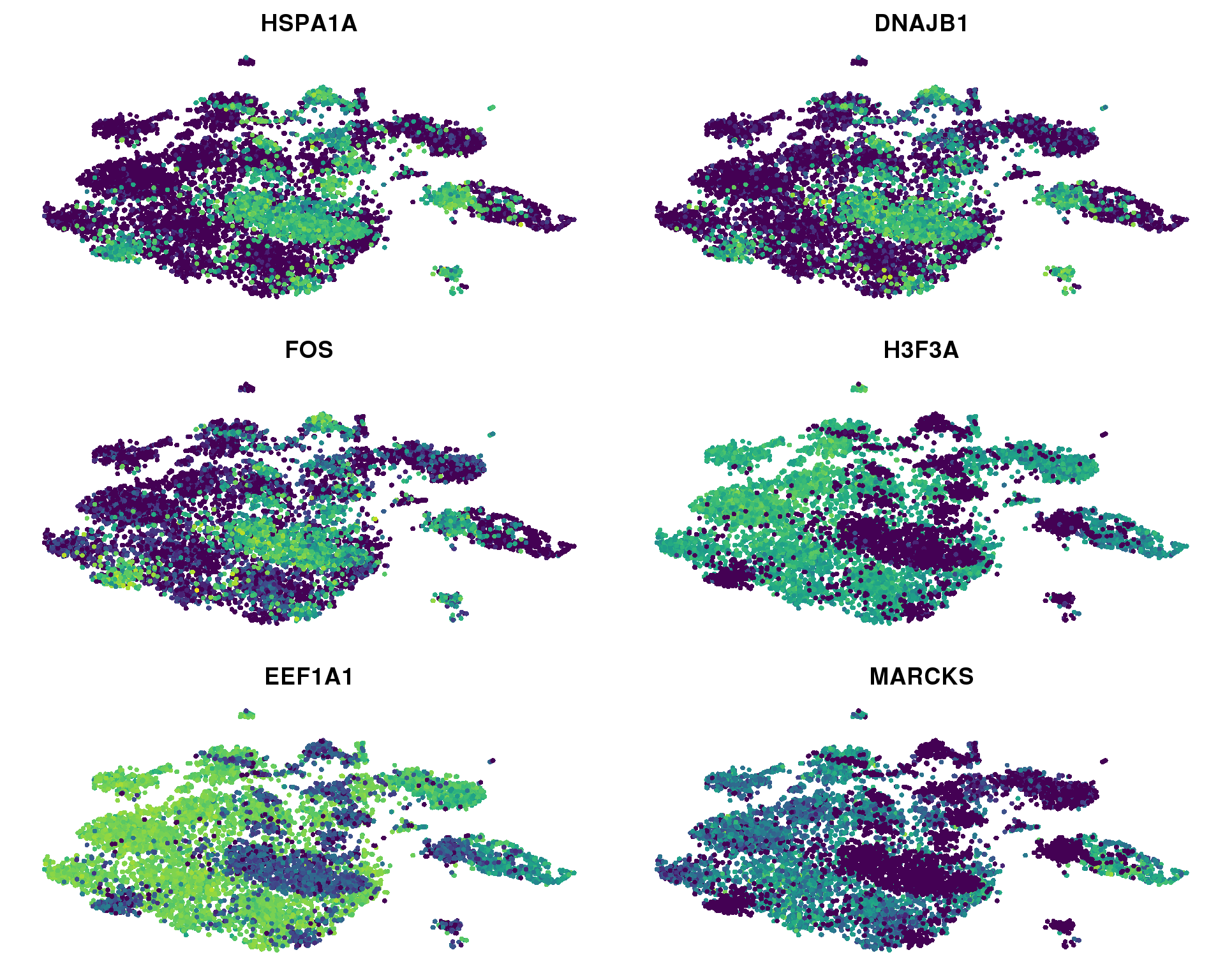
Expand here to see past versions of feature-plots-1.png:
| Version | Author | Date |
|---|---|---|
| 5476164 | Luke Zappia | 2018-08-10 |
Heat shock response
hs.genes <- read_tsv(here("data/response_to_heat_shock_BP.txt"),
col_names = c("gene", "description"),
col_types = cols(
gene = col_character(),
description = col_character()
))
fc <- de$avg_logFC
idx <- rownames(de) %in% hs.genes$gene
barcodeplot(fc, idx)
idx <- rownames(combined@data) %in% hs.genes$gene
group.fac <- factor(combined@meta.data$Group,
levels = c("Organoid", "Lindstrom"))
des.mat <- cbind(Intercept = 1, Group = as.numeric(group.fac) - 1)
roast.res <- roast(combined@data, idx, des.mat)A ROAST test for this gene set testing for up-regulation in the Lindstrom data gives a p-value of 5.002501310^{-4}.
Summary
Parameters
This table describes parameters used and set in this document.
params <- toJSON(list(
list(
Parameter = "resolutions",
Value = resolutions,
Description = "Range of possible clustering resolutions"
),
list(
Parameter = "res",
Value = res,
Description = "Selected resolution parameter for clustering"
),
list(
Parameter = "n.clusts",
Value = n.clusts,
Description = "Number of clusters produced by selected resolution"
),
list(
Parameter = "skipped",
Value = paste(seq(0, n.clusts - 1))[skip],
Description = "Clusters skipped for conserved marker and DE testing"
),
list(
Parameter = "n.sig",
Value = length(de.sig),
Description = "Number of genes in the group DE signature"
)
), pretty = TRUE)
kable(fromJSON(params))| Parameter | Value | Description |
|---|---|---|
| resolutions | c(0, 0.1, 0.2, 0.3, 0.4, 0.5, 0.6, 0.7, 0.8, 0.9, 1) | Range of possible clustering resolutions |
| res | 0.5 | Selected resolution parameter for clustering |
| n.clusts | 16 | Number of clusters produced by selected resolution |
| skipped | c(“14”, “15”) | Clusters skipped for conserved marker and DE testing |
| n.sig | 374 | Number of genes in the group DE signature |
Output files
This table describes the output files produced by this document. Right click and Save Link As… to download the results.
write_rds(combined, here("data/processed/Combined_clustered.Rds"))expr <- AverageExpression(combined, show.progress = FALSE) %>%
rename_all(function(x) {paste0("Mean", x)}) %>%
rownames_to_column("Gene")
prop <- AverageDetectionRate(combined) %>%
rename_all(function(x) {paste0("Prop", x)}) %>%
rownames_to_column("Gene")
alt.cols <- c(rbind(colnames(prop), colnames(expr)))[-1]
cluster.expr <- expr %>%
left_join(prop, by = "Gene") %>%
select(alt.cols)
cluster.assign <- combined@meta.data %>%
select(Cell, Dataset, Sample, Barcode, Cluster)dir.create(here("output", DOCNAME), showWarnings = FALSE)
write_lines(params, here("output", DOCNAME, "parameters.json"))
write_csv(cluster.assign, here("output", DOCNAME, "cluster_assignments.csv"))
write_csv(cluster.expr, here("output", DOCNAME, "cluster_expression.csv"))
writeGeneTable(markers, here("output", DOCNAME, "markers.csv"))
writeGeneTable(markers.list, here("output", DOCNAME, "markers.xlsx"))
writeGeneTable(con.markers, here("output", DOCNAME, "conserved_markers.csv"))
writeGeneTable(con.markers.list,
here("output", DOCNAME, "conserved_markers.xlsx"))
writeGeneTable(cluster.de, here("output", DOCNAME, "cluster_de.csv"))
writeGeneTable(cluster.de.list, here("output", DOCNAME, "cluster_de.xlsx"))
writeGeneTable(de, here("output", DOCNAME, "group_de.csv"))
write_csv(data.frame(Gene = de.sig),
here("output", DOCNAME, "de_signature.csv"))
writeGeneTable(cluster.de.filt,
here("output", DOCNAME, "cluster_de_filtered.csv"))
writeGeneTable(cluster.de.list.filt,
here("output", DOCNAME, "cluster_de_filtered.xlsx"))
kable(data.frame(
File = c(
glue("[parameters.json]({getDownloadURL('parameters.json', DOCNAME)})"),
glue("[cluster_assignments.csv]",
"({getDownloadURL('cluster_assignments.csv', DOCNAME)})"),
glue("[cluster_expression.csv]",
"({getDownloadURL('cluster_expression.csv', DOCNAME)})"),
glue("[markers.csv]({getDownloadURL('markers.csv.zip', DOCNAME)})"),
glue("[markers.xlsx]({getDownloadURL('markers.xlsx', DOCNAME)})"),
glue("[conserved_markers.csv]",
"({getDownloadURL('conserved_markers.csv.zip', DOCNAME)})"),
glue("[conserved_markers.xlsx]",
"({getDownloadURL('conserved_markers.xlsx', DOCNAME)})"),
glue("[cluster_de.csv]",
"({getDownloadURL('cluster_de.csv.zip', DOCNAME)})"),
glue("[cluster_de.xlsx]",
"({getDownloadURL('cluster_de.xlsx', DOCNAME)})"),
glue("[group_de.csv]({getDownloadURL('group_de.csv.zip', DOCNAME)})"),
glue("[de_signature.csv]",
"({getDownloadURL('de_signature.csv', DOCNAME)})"),
glue("[cluster_de_filtered.csv]",
"({getDownloadURL('cluster_de_filtered.csv.zip', DOCNAME)})"),
glue("[cluster_de_filtered.xlsx]",
"({getDownloadURL('cluster_de_filtered.xlsx', DOCNAME)})")
),
Description = c(
"Parameters set and used in this analysis",
"Cluster assignments for each cell",
"Cluster expression for each gene",
"Results of marker gene testing in CSV format",
paste("Results of marker gene testing in XLSX format with one tab",
"per cluster"),
"Results of conserved marker gene testing in CSV format",
paste("Results of conserved marker gene testing in XLSX format with",
"one tab per cluster"),
paste("Results of within cluster differential expression testing",
"in CSV format"),
paste("Results of within cluster differential expression testing",
"in XLSX format with one cluster per tab"),
paste("Results of between group differential expression testing",
"in CSV format"),
"Between group differential expression signature genes",
paste("Results of within cluster differential expression testing",
"after removing group DE signature in CSV format"),
paste("Results of within cluster differential expression testing",
"after removing group DE signature in XLSX format with one",
"cluster per tab")
)
)
)| File | Description |
|---|---|
| parameters.json | Parameters set and used in this analysis |
| cluster_assignments.csv | Cluster assignments for each cell |
| cluster_expression.csv | Cluster expression for each gene |
| markers.csv | Results of marker gene testing in CSV format |
| markers.xlsx | Results of marker gene testing in XLSX format with one tab per cluster |
| conserved_markers.csv | Results of conserved marker gene testing in CSV format |
| conserved_markers.xlsx | Results of conserved marker gene testing in XLSX format with one tab per cluster |
| cluster_de.csv | Results of within cluster differential expression testing in CSV format |
| cluster_de.xlsx | Results of within cluster differential expression testing in XLSX format with one cluster per tab |
| group_de.csv | Results of between group differential expression testing in CSV format |
| de_signature.csv | Between group differential expression signature genes |
| cluster_de_filtered.csv | Results of within cluster differential expression testing after removing group DE signature in CSV format |
| cluster_de_filtered.xlsx | Results of within cluster differential expression testing after removing group DE signature in XLSX format with one cluster per tab |
Session information
devtools::session_info() setting value
version R version 3.5.0 (2018-04-23)
system x86_64, linux-gnu
ui X11
language (EN)
collate en_US.UTF-8
tz Australia/Melbourne
date 2018-12-05
package * version date source
abind 1.4-5 2016-07-21 cran (@1.4-5)
acepack 1.4.1 2016-10-29 cran (@1.4.1)
ape 5.1 2018-04-04 cran (@5.1)
assertthat 0.2.0 2017-04-11 CRAN (R 3.5.0)
backports 1.1.2 2017-12-13 CRAN (R 3.5.0)
base * 3.5.0 2018-06-18 local
base64enc 0.1-3 2015-07-28 CRAN (R 3.5.0)
bibtex 0.4.2 2017-06-30 cran (@0.4.2)
bindr 0.1.1 2018-03-13 cran (@0.1.1)
bindrcpp 0.2.2 2018-03-29 cran (@0.2.2)
BiocParallel * 1.14.2 2018-07-08 Bioconductor
bitops 1.0-6 2013-08-17 cran (@1.0-6)
broom 0.5.0 2018-07-17 cran (@0.5.0)
caret 6.0-80 2018-05-26 cran (@6.0-80)
caTools 1.17.1.1 2018-07-20 cran (@1.17.1.)
cellranger 1.1.0 2016-07-27 CRAN (R 3.5.0)
checkmate 1.8.5 2017-10-24 cran (@1.8.5)
class 7.3-14 2015-08-30 CRAN (R 3.5.0)
cli 1.0.0 2017-11-05 CRAN (R 3.5.0)
cluster 2.0.7-1 2018-04-13 CRAN (R 3.5.0)
clustree * 0.2.2.9000 2018-08-01 Github (lazappi/clustree@66a865b)
codetools 0.2-15 2016-10-05 CRAN (R 3.5.0)
colorspace 1.3-2 2016-12-14 cran (@1.3-2)
compiler 3.5.0 2018-06-18 local
cowplot * 0.9.3 2018-07-15 cran (@0.9.3)
crayon 1.3.4 2017-09-16 CRAN (R 3.5.0)
CVST 0.2-2 2018-05-26 cran (@0.2-2)
data.table 1.11.4 2018-05-27 cran (@1.11.4)
datasets * 3.5.0 2018-06-18 local
ddalpha 1.3.4 2018-06-23 cran (@1.3.4)
DEoptimR 1.0-8 2016-11-19 cran (@1.0-8)
devtools 1.13.6 2018-06-27 CRAN (R 3.5.0)
diffusionMap 1.1-0.1 2018-07-21 cran (@1.1-0.1)
digest 0.6.15 2018-01-28 CRAN (R 3.5.0)
dimRed 0.1.0 2017-05-04 cran (@0.1.0)
diptest 0.75-7 2016-12-05 cran (@0.75-7)
doSNOW 1.0.16 2017-12-13 cran (@1.0.16)
dplyr * 0.7.6 2018-06-29 cran (@0.7.6)
DRR 0.0.3 2018-01-06 cran (@0.0.3)
dtw 1.20-1 2018-05-18 cran (@1.20-1)
evaluate 0.10.1 2017-06-24 CRAN (R 3.5.0)
fitdistrplus 1.0-9 2017-03-24 cran (@1.0-9)
flexmix 2.3-14 2017-04-28 cran (@2.3-14)
FNN 1.1 2013-07-31 cran (@1.1)
forcats * 0.3.0 2018-02-19 CRAN (R 3.5.0)
foreach 1.4.4 2017-12-12 cran (@1.4.4)
foreign 0.8-71 2018-07-20 CRAN (R 3.5.0)
Formula 1.2-3 2018-05-03 cran (@1.2-3)
fpc 2.1-11.1 2018-07-20 cran (@2.1-11.)
gbRd 0.4-11 2012-10-01 cran (@0.4-11)
gdata 2.18.0 2017-06-06 cran (@2.18.0)
geometry 0.3-6 2015-09-09 cran (@0.3-6)
ggforce 0.1.3 2018-07-07 CRAN (R 3.5.0)
ggplot2 * 3.0.0 2018-07-03 cran (@3.0.0)
ggraph * 1.0.2 2018-07-07 CRAN (R 3.5.0)
ggrepel 0.8.0 2018-05-09 CRAN (R 3.5.0)
ggridges 0.5.0 2018-04-05 cran (@0.5.0)
git2r 0.21.0 2018-01-04 CRAN (R 3.5.0)
glue * 1.3.0 2018-07-17 cran (@1.3.0)
gower 0.1.2 2017-02-23 cran (@0.1.2)
gplots 3.0.1 2016-03-30 cran (@3.0.1)
graphics * 3.5.0 2018-06-18 local
grDevices * 3.5.0 2018-06-18 local
grid 3.5.0 2018-06-18 local
gridExtra 2.3 2017-09-09 cran (@2.3)
gtable 0.2.0 2016-02-26 cran (@0.2.0)
gtools 3.8.1 2018-06-26 cran (@3.8.1)
haven 1.1.2 2018-06-27 CRAN (R 3.5.0)
here * 0.1 2017-05-28 CRAN (R 3.5.0)
Hmisc 4.1-1 2018-01-03 cran (@4.1-1)
hms 0.4.2 2018-03-10 CRAN (R 3.5.0)
htmlTable 1.12 2018-05-26 cran (@1.12)
htmltools 0.3.6 2017-04-28 CRAN (R 3.5.0)
htmlwidgets 1.2 2018-04-19 cran (@1.2)
httr 1.3.1 2017-08-20 CRAN (R 3.5.0)
ica 1.0-2 2018-05-24 cran (@1.0-2)
igraph 1.2.2 2018-07-27 cran (@1.2.2)
ipred 0.9-6 2017-03-01 cran (@0.9-6)
irlba 2.3.2 2018-01-11 cran (@2.3.2)
iterators 1.0.10 2018-07-13 cran (@1.0.10)
jsonlite * 1.5 2017-06-01 CRAN (R 3.5.0)
kernlab 0.9-26 2018-04-30 cran (@0.9-26)
KernSmooth 2.23-15 2015-06-29 CRAN (R 3.5.0)
knitr * 1.20 2018-02-20 CRAN (R 3.5.0)
lars 1.2 2013-04-24 cran (@1.2)
lattice 0.20-35 2017-03-25 CRAN (R 3.5.0)
latticeExtra 0.6-28 2016-02-09 cran (@0.6-28)
lava 1.6.2 2018-07-02 cran (@1.6.2)
lazyeval 0.2.1 2017-10-29 cran (@0.2.1)
limma * 3.36.2 2018-06-21 Bioconductor
lmtest 0.9-36 2018-04-04 cran (@0.9-36)
lubridate 1.7.4 2018-04-11 cran (@1.7.4)
magic 1.5-8 2018-01-26 cran (@1.5-8)
magrittr 1.5 2014-11-22 CRAN (R 3.5.0)
MASS 7.3-50 2018-04-30 CRAN (R 3.5.0)
Matrix * 1.2-14 2018-04-09 CRAN (R 3.5.0)
mclust 5.4.1 2018-06-27 cran (@5.4.1)
memoise 1.1.0 2017-04-21 CRAN (R 3.5.0)
metap 1.0 2018-07-25 cran (@1.0)
methods * 3.5.0 2018-06-18 local
mixtools 1.1.0 2017-03-10 cran (@1.1.0)
ModelMetrics 1.1.0 2016-08-26 cran (@1.1.0)
modelr 0.1.2 2018-05-11 CRAN (R 3.5.0)
modeltools 0.2-22 2018-07-16 cran (@0.2-22)
munsell 0.5.0 2018-06-12 cran (@0.5.0)
mvtnorm 1.0-8 2018-05-31 cran (@1.0-8)
nlme 3.1-137 2018-04-07 CRAN (R 3.5.0)
nnet 7.3-12 2016-02-02 CRAN (R 3.5.0)
parallel 3.5.0 2018-06-18 local
pbapply 1.3-4 2018-01-10 cran (@1.3-4)
pillar 1.3.0 2018-07-14 cran (@1.3.0)
pkgconfig 2.0.1 2017-03-21 cran (@2.0.1)
pls 2.6-0 2016-12-18 cran (@2.6-0)
plyr 1.8.4 2016-06-08 cran (@1.8.4)
png 0.1-7 2013-12-03 cran (@0.1-7)
prabclus 2.2-6 2015-01-14 cran (@2.2-6)
prodlim 2018.04.18 2018-04-18 cran (@2018.04)
proxy 0.4-22 2018-04-08 cran (@0.4-22)
purrr * 0.2.5 2018-05-29 cran (@0.2.5)
R.methodsS3 1.7.1 2016-02-16 CRAN (R 3.5.0)
R.oo 1.22.0 2018-04-22 CRAN (R 3.5.0)
R.utils 2.6.0 2017-11-05 CRAN (R 3.5.0)
R6 2.2.2 2017-06-17 CRAN (R 3.5.0)
ranger 0.10.1 2018-06-04 cran (@0.10.1)
RANN 2.6 2018-07-16 cran (@2.6)
RColorBrewer 1.1-2 2014-12-07 cran (@1.1-2)
Rcpp 0.12.18 2018-07-23 cran (@0.12.18)
RcppRoll 0.3.0 2018-06-05 cran (@0.3.0)
Rdpack 0.8-0 2018-05-24 cran (@0.8-0)
readr * 1.1.1 2017-05-16 CRAN (R 3.5.0)
readxl 1.1.0 2018-04-20 CRAN (R 3.5.0)
recipes 0.1.3 2018-06-16 cran (@0.1.3)
reshape2 1.4.3 2017-12-11 cran (@1.4.3)
reticulate 1.9 2018-07-06 cran (@1.9)
rlang 0.2.1 2018-05-30 CRAN (R 3.5.0)
rmarkdown 1.10.2 2018-07-30 Github (rstudio/rmarkdown@18207b9)
robustbase 0.93-2 2018-07-27 cran (@0.93-2)
ROCR 1.0-7 2015-03-26 cran (@1.0-7)
rpart 4.1-13 2018-02-23 CRAN (R 3.5.0)
rprojroot 1.3-2 2018-01-03 CRAN (R 3.5.0)
rstudioapi 0.7 2017-09-07 CRAN (R 3.5.0)
Rtsne 0.13 2017-04-14 cran (@0.13)
rvest 0.3.2 2016-06-17 CRAN (R 3.5.0)
scales 0.5.0 2017-08-24 cran (@0.5.0)
scatterplot3d 0.3-41 2018-03-14 cran (@0.3-41)
SDMTools 1.1-221 2014-08-05 cran (@1.1-221)
segmented 0.5-3.0 2017-11-30 cran (@0.5-3.0)
Seurat * 2.3.1 2018-05-05 url
sfsmisc 1.1-2 2018-03-05 cran (@1.1-2)
snow 0.4-2 2016-10-14 cran (@0.4-2)
splines 3.5.0 2018-06-18 local
stats * 3.5.0 2018-06-18 local
stats4 3.5.0 2018-06-18 local
stringi 1.2.4 2018-07-20 cran (@1.2.4)
stringr * 1.3.1 2018-05-10 CRAN (R 3.5.0)
survival 2.42-6 2018-07-13 CRAN (R 3.5.0)
tclust 1.4-1 2018-05-24 cran (@1.4-1)
tibble * 1.4.2 2018-01-22 cran (@1.4.2)
tidyr * 0.8.1 2018-05-18 cran (@0.8.1)
tidyselect 0.2.4 2018-02-26 cran (@0.2.4)
tidyverse * 1.2.1 2017-11-14 CRAN (R 3.5.0)
timeDate 3043.102 2018-02-21 cran (@3043.10)
tools 3.5.0 2018-06-18 local
trimcluster 0.1-2.1 2018-07-20 cran (@0.1-2.1)
tsne 0.1-3 2016-07-15 cran (@0.1-3)
tweenr 0.1.5 2016-10-10 CRAN (R 3.5.0)
units 0.6-0 2018-06-09 CRAN (R 3.5.0)
utils * 3.5.0 2018-06-18 local
VGAM 1.0-5 2018-02-07 cran (@1.0-5)
viridis * 0.5.1 2018-03-29 cran (@0.5.1)
viridisLite * 0.3.0 2018-02-01 cran (@0.3.0)
whisker 0.3-2 2013-04-28 CRAN (R 3.5.0)
withr 2.1.2 2018-03-15 CRAN (R 3.5.0)
workflowr 1.1.1 2018-07-06 CRAN (R 3.5.0)
writexl * 1.0 2018-05-10 CRAN (R 3.5.0)
xml2 1.2.0 2018-01-24 CRAN (R 3.5.0)
yaml 2.2.0 2018-07-25 cran (@2.2.0)
zoo 1.8-3 2018-07-16 cran (@1.8-3) This reproducible R Markdown analysis was created with workflowr 1.1.1